Aplicaciones de edo’s de 2do orden a oscilaciones

Dr. Mario Medina Valdez

m=masa del objeto a= resistencia del medio

k=constante del resorte F(t)=fuerzas externas

a=0 movimiento no amortiguadoa no nulo, movimiento amortiguado

F(t)=0, movimiento libreF(t) no nulo, movimiento forzado

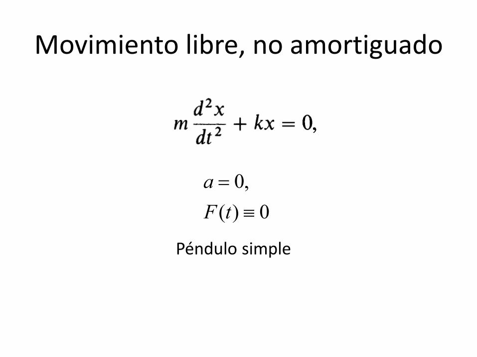
Movimiento libre, no amortiguado

0,( ) 0

aF t=

≡

Péndulo simple

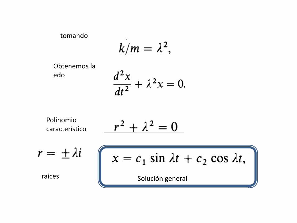
tomando

Obtenemos la edo

Polinomio característico

raíces Solución general

Usando las condiciones iniciales

Y la derivada de la solución

Obtenemos los valores de las constantes

De esta forma

Reescribiremos la solución para obtener mayor información de la misma

donde

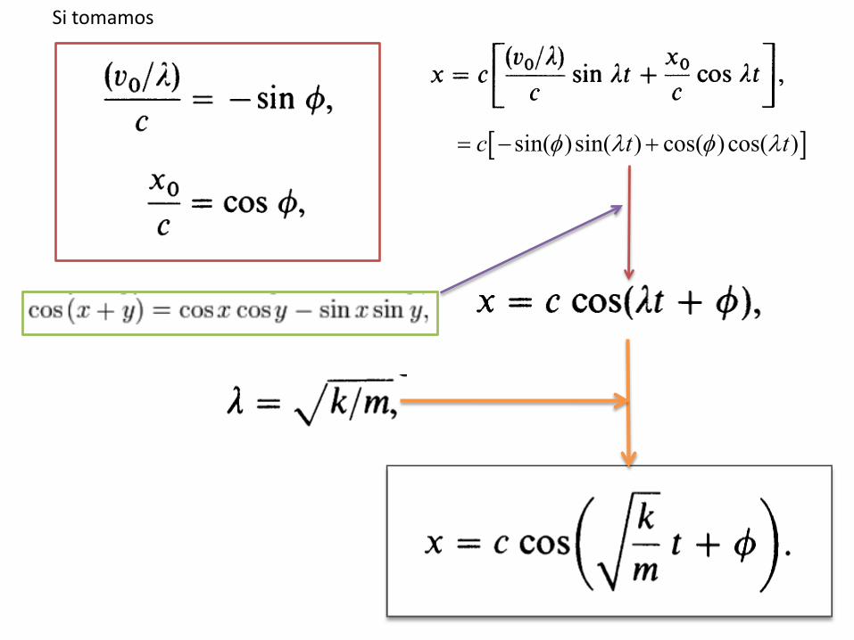
[ ]sin( )sin( ) cos( ) cos( )c t tφ λ φ λ= − +

Si tomamos

Movimiento armónico simple

c

-c

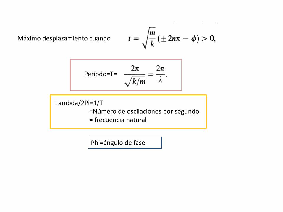
Máximo desplazamiento cuando

Phi=ángulo de fase

Lambda/2Pi=1/T=Número de oscilaciones por segundo= frecuencia natural

Período=T=

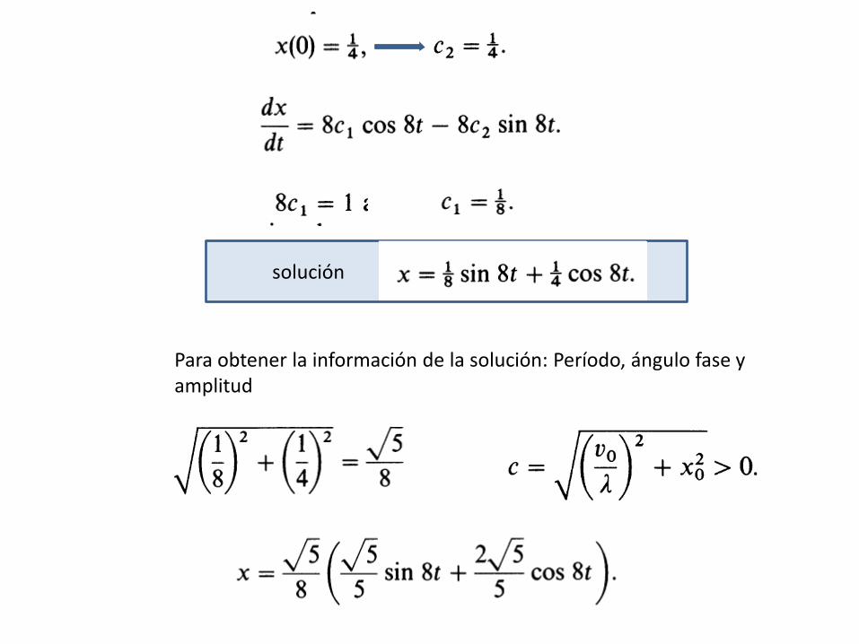
solución

Para obtener la información de la solución: Período, ángulo fase y amplitud

Amplitud=

Período=T=

Frecuencia=

Solución

Movimiento libre, amortiguado

Las raíces dependen del sigo del discriminante

1er caso: Movimiento libre amortiguado:

Raíces:

Solución general:

1er caso: Movimiento libre amortiguado

Raíces complejas:

Solución general:

Una mejor forma de escribir la solución:

Factor de amortiguamiento

Movimiento periódico oscilatorio

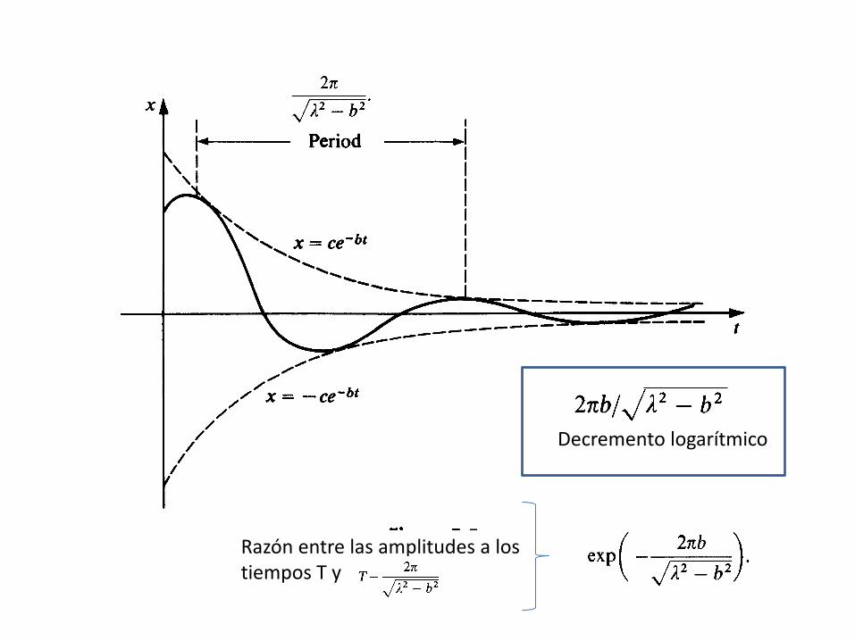
Decremento logarítmico

Razón entre las amplitudes a los tiempos T y

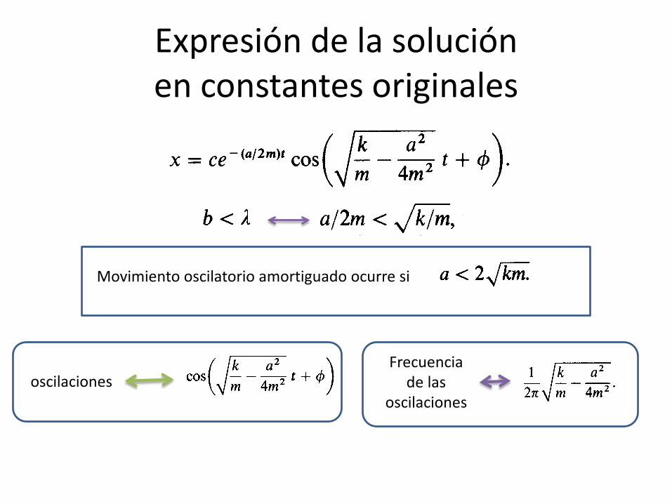
Expresión de la solución en constantes originales

Movimiento oscilatorio amortiguado ocurre si

oscilacionesFrecuencia

de las oscilaciones

Si no hay resistencia del medio, a=0

Frecuencia natural del sistema sin fricción

La frecuencia natural de las oscilaciones en un sistema oscilatorio con fricción es menor

que la frecuencia natural del correspondiente sistema sin fricción

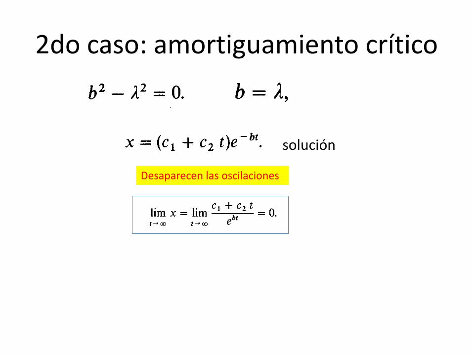
2do caso: amortiguamiento crítico

solución

Desaparecen las oscilaciones

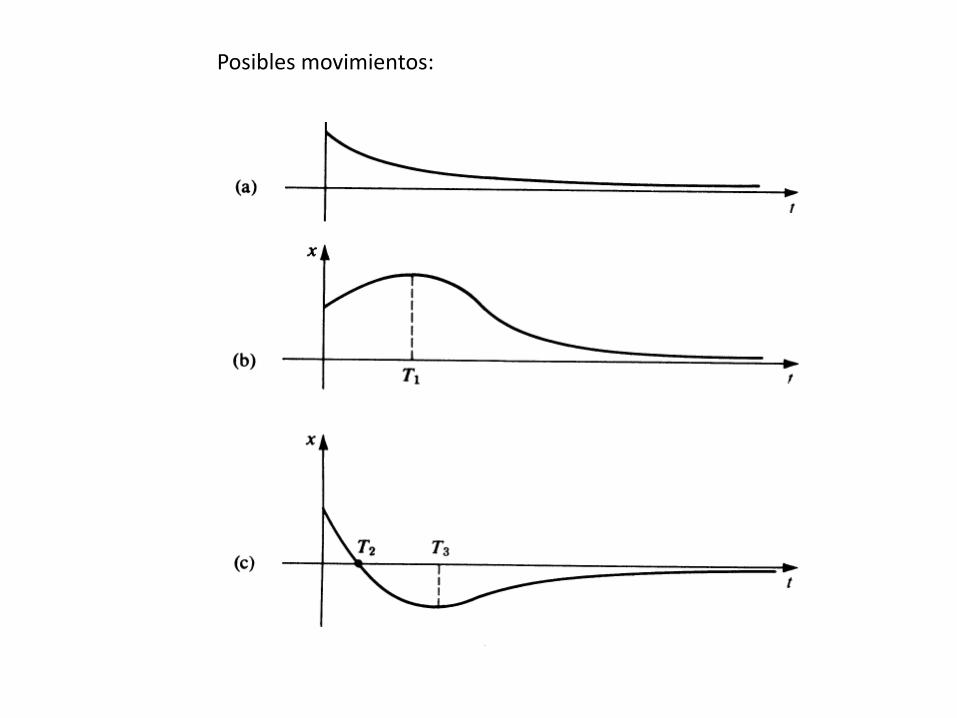
Posibles movimientos:

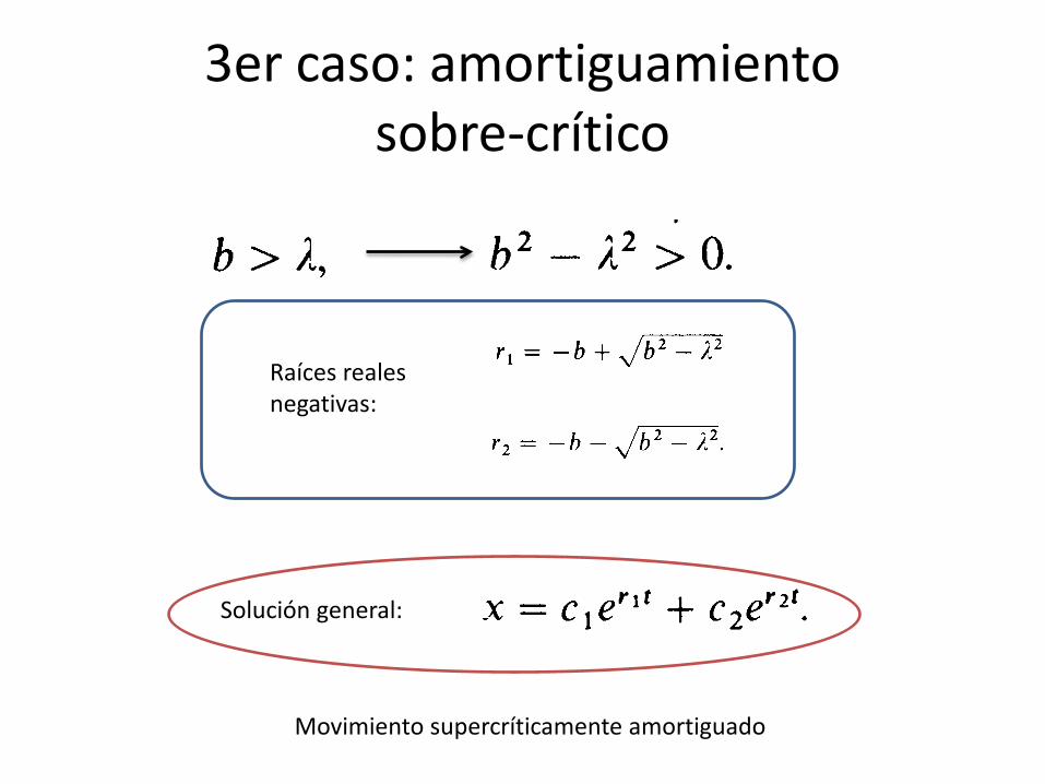
3er caso: amortiguamiento sobre-crítico

Raíces reales negativas:

Solución general:

Movimiento supercríticamente amortiguado

Ejemplos

Peso=

solución Otra forma de escribirla

Factor de amortiguamiento “Período”

323π

Decremento logarítmico

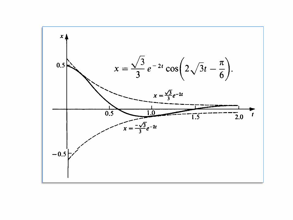
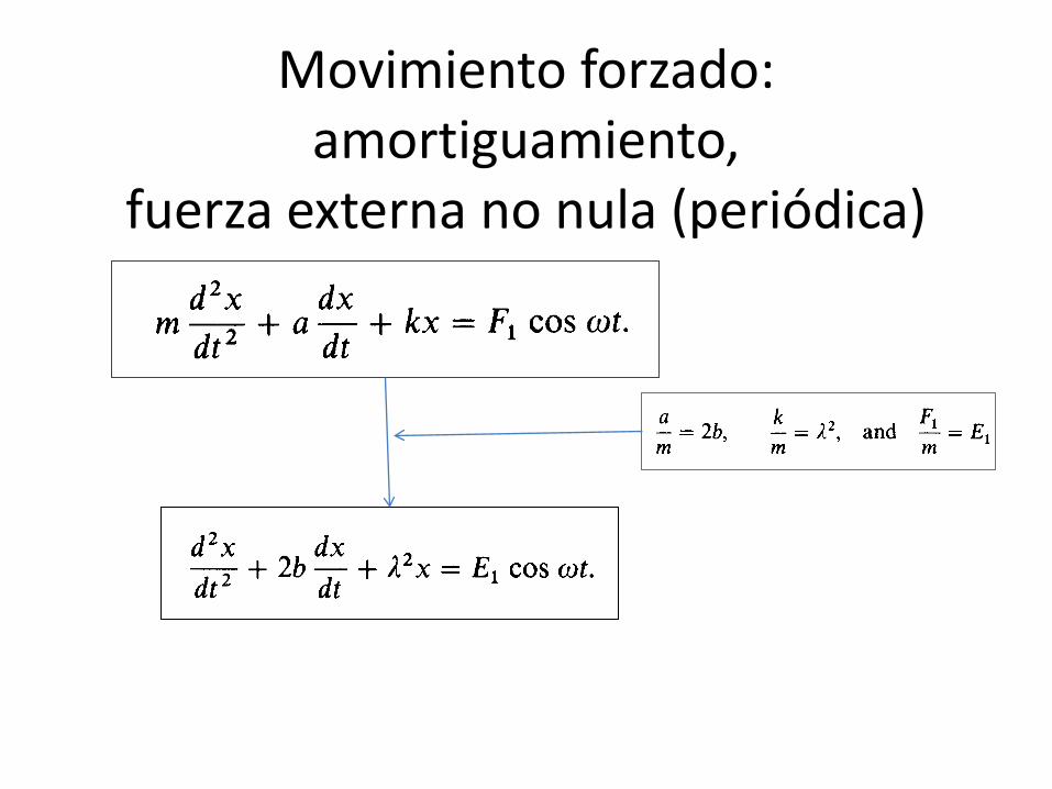
Movimiento forzado: amortiguamiento,

fuerza externa no nula (periódica)

Supongamos un término de amortiguamiento pequeño, es decir, el amortiguamiento es menor que crítico :

Solución particular

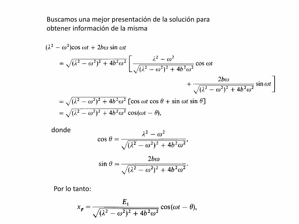
donde

Por lo tanto:

Buscamos una mejor presentación de la solución para obtener información de la misma

Solución general:

Solución amortiguada en ausencia de fuerzas externas

Resulta de la presencia de la fuerza externa, representa un movimiento armónico simple de período

Solución de estado estacionarioTiende a anularse para t’ssuficientemente grandes

Sol’n general de la homogénea

Solución part. De la forma

Así:

Solución general:

derivando

Usando condiciones iniciales

Obtenemos la solución

Calculando derivada primera, segunda y sustituyendo en la edo no homogénea

usando

con

Por otra parte

donde

En consecuenciaSol’n edoestacionario

Solución estado estacionario

Solución del problema

TRANSFORMADA DE LAPLACESegundo teorema de traslación

Ejemplo: calcular

0

0

( ) ( )

( ) ( ) ( ) ( )

st

ast st

a

e g t U t a dt

g t e U t a dt g t e U t a dt

∞−

∞− −

− =

− + − =

∫

∫ ∫

Ejemplo: resolver EDO’s usando transformada de Laplace

Observemos que

Aplicando TLa la edo original

Un poco de álgebra

Despejando Y(s)

Necesitamos calcular tres transformadas inversas deLaplace

2

2 2

( 1)( 1)

1 1 1

ss s

A B Css s s

=+ +

+ ++ + +

1

1( ) , ( ) 1

( ( ) ) ( ) ( )

t

s

F s f t es

L F s e f t U tπ π π

−

− −

= =+

= − −

Identidades trigonométricas

2

1 12

1

1 ( ) ,1

1( ) ( ( )) ( ) sin( )1

( ( ) ) ( ) ( )

s s

s

e F s es

f t L F s L ts

L F s e f t U t

π π

π π π

− −

− −

− −

=+

= = =+

= − −

2

1 12

1

( ) ,1

( ) ( ( )) ( ) cos( )1

( ( ) ) ( ) ( )

s s

s

s e F s es

sf t L F s L ts

L F s e f t U t

π π

π π π

− −

− −

− −

=+

= = =+

= − −

Finalmente

Derivadas de Transformada de LaplaceConsideremos la derivada con respecto a s de la transformada de Laplace F(S) de f(t)

en consecuencia, tenemos que

( )

dF sds

= −

donde F(s)=L(f(t))

Más generalmente

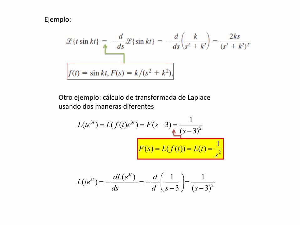
Ejemplo:

Otro ejemplo: cálculo de transformada de Laplaceusando dos maneras diferentes

3 32

1( ) ( ( ) ) ( 3)( 3)

t tL te L f t e F ss

= = − =−

2

1( ) ( ( )) ( )F s L f t L ts

= = =

33

2

( ) 1 1( ) 3 ( 3)

tt dL e dL te

ds d s s = − = − = − −

Ejemplo edo 2do orden coef ctes no homogénea

( )

( )

22

22

22

22 2

( '') 16 ( ) (cos(4 ))

( ) (0) '(0) 16 ( )16

( ) 1 16 ( )16

16 ( ) 116

1( )16 16

L x L x L tss X s sx x X s

sss X s X s

sss X s

ssX s

s s

+ =

− − + =+

− + =+

+ = ++

= ++ +

Aplicando transf. de Laplace y propiedades

( )( ) ( )

1 1 1 12 22 22 2

1 1( ) ( )16 1616 16

s sx t L X s L L Ls ss s

− − − −

= = + = + + + + +

De esta forma:

Sabemos que k=4

Finalmente obtenemos la solución buscada, usando viejos “trucos” algebraicos de multiplicar y dividir por el mismo número

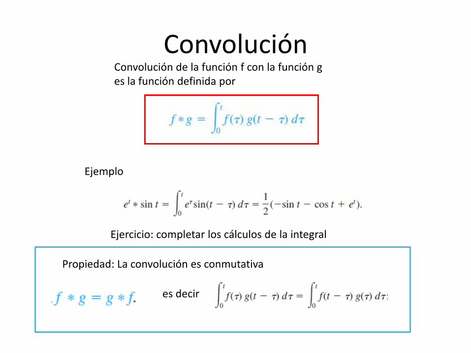
ConvoluciónConvolución de la función f con la función g es la función definida por

Ejemplo

Ejercicio: completar los cálculos de la integral

Propiedad: La convolución es conmutativa

es decir

U(t-a)-U(t-b)

Convolución de dos gaussianas

Propiedades convolución

Teorema de convolución

Para f(t) y g(t) continuas a trozos y de orden exponencial

( )1 ( ) ( )f g L F s G s−∗ = cuando

( )

( )

1

1

( ) ( )

( ) ( )

f t L F s

g t L G s

−

−

=

=

Versión “retro”:

El Teorema de convolución permite calcular transf de Laplace inversas de

productos de funciones que dependen de la variable “s”

( ) , ( ) sin( )tf t e g t t= =

Ejemplo: Calcular la transformada de una convolución de dos funciones

Otro ejemplo: calcular la transformada de inversa de Laplace de un producto de dos funciones

( ) ( ) 0 0 01 1 122

0 0 0

a) ( ) ( ) 1 sin( ) sin( )1 1 1 ( ) ( )

11 b) ( ) ( ) sin( ) 1 sin( ) 1 cos( )

t t t

t t t

f g f g t d t d t dL L L F s G s f g

s ss sg f g f t d d d t

τ τ τ τ τ τ τ

τ τ τ τ τ τ τ

− − −

∗ = − = ⋅ − = − = = ⋅ = = ∗ = ++ ∗ = − = ⋅ = = −

∫ ∫ ∫

∫ ∫ ∫

( )

1

12 2

1 1( ) , 1 ( )

1 1( ) , sin ( )1 1

F s L f ts s

G s L t g ts s

−

−

= = =

= = = + +

( )1 1 12 2

0

0

1 1 1 ( ) ( ) ( ) ( )( 1)( 1) 1 1

sin( ) sin( ) ... sin( )

sin( ) sin( ) ...

tt

tt

t t

L L L F s G s f t g ts s s s

e t e t d blablablae t

t e e d blablabla

τ

τ

τ τ

τ τ

− − −

−

= ⋅ = ⋅ = ∗ − + − +

∗ = − == ∗ = ∗ = =

∫

∫

Otro ejemplo del uso del Teorema de Convolución para el cálculo de transformadas inversas de Laplace:

Funciones periódicas

f(t):[0,infinito)R, periódica de período T, continua por trozos y de orden exponencial

DemostraciónLa transf de Laplace se divide en dos integrales

Con el cambio de variables

Por consiguiente

Con un poco de algebrita podemos despejar la transformada deseada

SOLUCIÓN NUMÉRICA DE

ECUACIONES DIFERENCIALES ORDINARIAS DE PRIMER ORDEN

SOLUCION NUMERICA

Una solución de esta ecuación inicial con CI es una función

0 0: ( , )x xϕ ε ε− + →

tal que

0 0'( ) ( , ( )), para ( , )x f x x x x xϕ ϕ ε ε= ∈ − +

PROBLEMA: Hallar una aproximación numérica de la solución de la EDO con CI

Curva solución

pendiente

Campo de pendientes f(x,y)

0 1 2 ,na x x x x b= < < < < =

Conocemos 0( ) ( )a xϕ ϕ=

Queremos obtener una aproximación de ( ) para b b aϕ >

Consideramos una partición del intervalo

donde lo llamamos tamaño de paso. Observemos que

[ , ]a b

1i it thn

+ −=

0 , 1, 2,...kt kh t k n= + =

Curva solución

pendiente=

Consideramos la condición inicial

0 0 0 0( , ) ( , ( )) ( , ( ))x y x y x a y a= =

0 0 0 2( ) ( ) '( )( ) ( )y x y x y x x x R x= + − +

El desarrollo de Taylor 1er orden alrededor de 0x

0 0 0( ) ( ) '( )( )y x y x y x x x+ −

obtenemos la aproximación lineal de ( )y xcerca de 0x

tomando 1 0x x x h= = +

obtenemos1 0 0 0 0 0 0( ) ( ) ( ) ( ) '( ) ( ) ( , )y x y x y x h y x y x h y x f x y h= = + + = +

1 1 0 0 0

0 0 0

( ) ( ) ( , ) = ( , )y y x y x f x y h

y f x y h= +

+

En resumen:

En general, tenemos

1 1( ) ( ) ( , ) = ( , )

k k k k k

k k k

y y x y x f x y hy f x y h

+ += ++

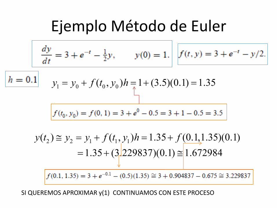
Ejemplo Método de Euler

1 0 0 0( , ) 1 (3.5)(0.1) 1.35y y f t y h= + = + =

2 2 1 1 1( ) ( , ) 1.35 (0.1,1.35)(0.1) 1.35 (3.229837)(0.1) 1.672984y t y y f t y h f≅ = + = +

= + ≅

SI QUEREMOS APROXIMAR y(1) CONTINUAMOS CON ESTE PROCESO

EjemploConsideremos la ecuación diferencial ordinaria

Recordemos que no es difícil encontrar la solución analítica, mediante el método de separación de variables, de la ecuación diferencial. Ejercicio: Hallar la solución analítica de la ecuación diferencial anterior

Veamos nuestro primer ejemplo para resolover ecuaciones diferenciales ordinarias de primer orden mediante Matlab:

function r = yexact(t,y0,K,s) r = y0*exp(K*t) + s*(1 - exp(K*t));

Se ha definido una función que depende de cuatro argumentos: el temporal, la condición inicial y dos constantes. Supongamos que sus valores están dados por y0=100, K=1, and s=20. Escribamos el siguiente código en nuestra pantalla del editor de Matlab:

El siguiente comando crea un vector

t = 0:0.01:5;

plot(t,yexact(t,100,1,20))

El siguiente comando crea la gráfica de la solución

Figura 1: Solución exacta

Paso 1. definir f (t, y)Paso 2. Entrada: Valores iniciales t0 and y0Paso 3. entrada tamaño de paso h # de pasos nPaso 4. salida t0 and y0Paso 5. para j de 1 a n doPaso 6. k1 = f (t, y)y = y + h ∗ k1

T = t + hPaso 7. salidas t y yPaso 8. end

Estructura computacional del Método de Euler

Programa en Matlabclc;clf;clear all;T=25;tinic=0.0;tfinal=5.0;yinic=50.0;n=100;f=@(t,y) -2*(y-T);h=(tfinal-tinic)/n;t=zeros(1,n+1);y=zeros(1,n+1);t(1)=tinic;y(1)=yinic;for i=1:n

t(i+1)=t(i)+h;y(i+1)=y(i)+h*f(t(i),y(i));

end

plot(t,y,'b')title('Soluciones de dy/dt=-2*(y-T), y(0)=T mediante Euler')axis([0 5 20 55])xlabel('Tiempo');ylabel('Temperatura')hold onplot(t,25,'-r')

Gráfica obtenida con Matlab

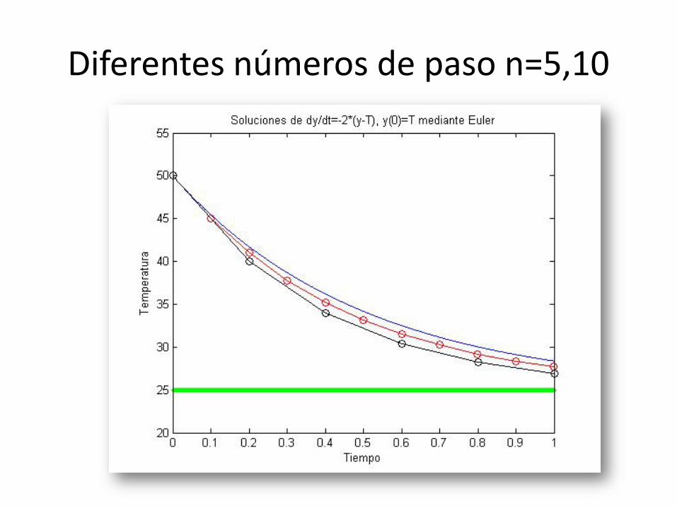
Diferentes números de paso n=5,10

function [t,y]=Euler_clasico(f,tinic,yinic,tfinal,n)h=(tfinal-tinic)/n;t=zeros(1,n+1);y=zeros(1,n+1);t(1)=tinic;y(1)=yinic;for i=1:n

t(i+1)=t(i)+h;y(i+1)=y(i)+h*f(t(i),y(i));

end

clc;clf;clear all;T=25;tinic=0.0;tfinal=5.0;yinic=50.0;n=100;f=@(t,y) -2*(y-T);[t1,y1]=Euler_clasico(f,tinic,yinic,tfinal,n);plot(t1,y1,'b')title('Soluciones de dy/dt=-2*(y-T), y(0)=T mediante Euler')axis([0 5 20 55])xlabel('Tiempo');ylabel('Temperatura')hold onplot(t1,25,'-r')

Programas Método de Euler en Matlab

TIPO FUNCIÓN

TIPO SCRIPT

%%%PROGRAMA DEL METODO DE EULER MODIFICADO CON UN ARCHIVO TIPO SCRIPT%%%%%%ECUACION DIFERENCIAL ORDINARIA dy/dt=k(y-c)%%%%

k = 1;c = 20;y0= 100;npuntos = 50; %%Numero de pasos%%h = 0.1;

y = zeros(npuntos,1); %Inicializamos el vector 'y' de posiciones con ceros%t = zeros(npuntos,1); %Inicializamos el vector 't' de tiempos con ceros%

y(1) = y0; %Posicion inicial%t(1) = 0.0; %Timepo inicial%

for j = 1 : npuntos %-1 % loop para el tamaño de paso%y(j+1) = y(j) + (h/2) * ((k*(y(j)-c)+ y(j) +h*k*(y(j)-c)));t(j+1) = t (j) + h;

end

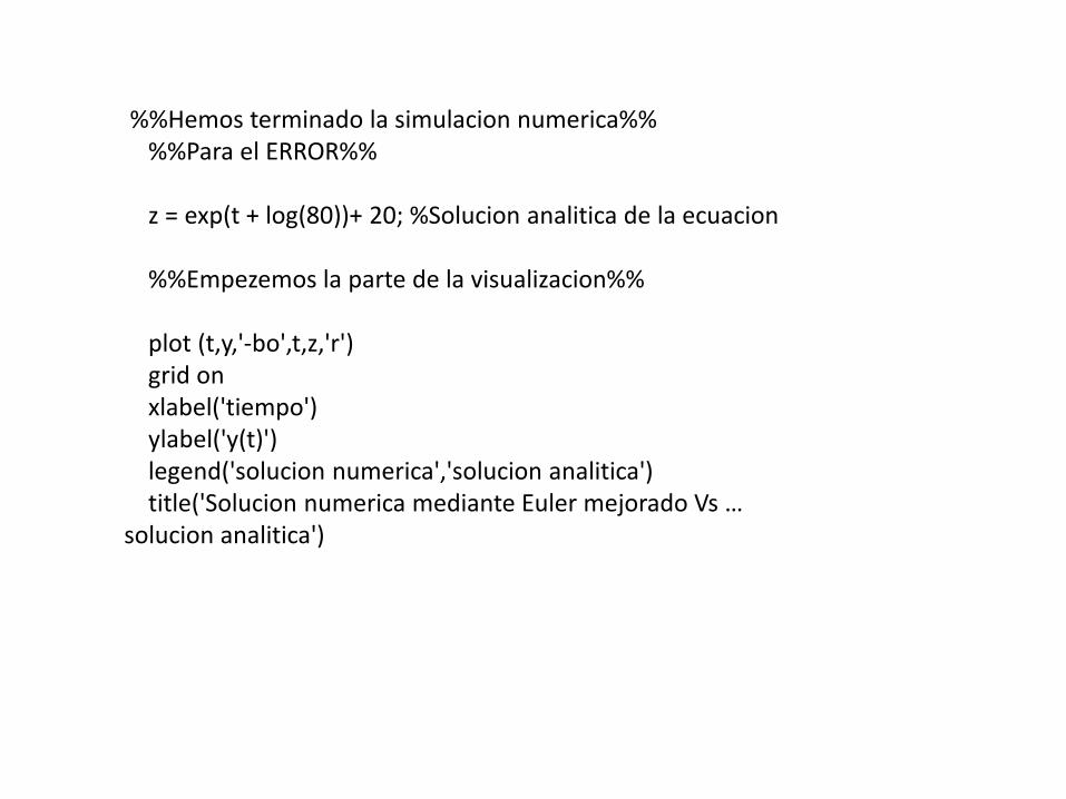
%%Hemos terminado la simulacion numerica%%%%Para el ERROR%%

z = exp(t + log(80))+ 20; %Solucion analitica de la ecuacion

%%Empezemos la parte de la visualizacion%%

plot (t,y,'-bo',t,z,'r')grid onxlabel('tiempo')ylabel('y(t)')legend('solucion numerica','solucion analitica')title('Solucion numerica mediante Euler mejorado Vs …

solucion analitica')

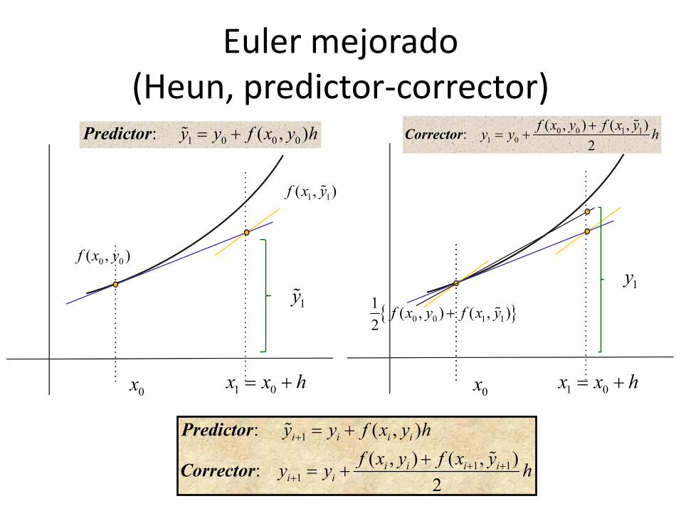
Euler mejorado (Heun, predictor-corrector)

0x 1 0x x h= +

1y

1 1( , )f x y

0 0( , )f x y

{ }0 0 1 11 ( , ) ( , )2

f x y f x y+

1y

1

1 11

: ( , )( , ) ( , ):

2

i i i i

i i i ii i

y y f x y hf x y f x yy y h

+

+ ++

= ++

= +

Predictor

Corrector

1 0 0 0: ( , )y y f x y h= +Predictor 0 0 1 11 0

( , ) ( , ):2

f x y f x yy y h+= +

Corrector

0x 1 0x x h= +

Ejemplo Euler-mejorado

Comparación Euler vs. Euler-mejorado

Estructura computacional del Método de Euler Mejorado

Paso 1. definir f (t, y)Paso 2. Entrada: Valores iniciales t0 and y0Paso 3. entrada tamaño de paso h # de pasos nPaso 4. salida t0 and y0Paso 5. para j de 1 a n doPaso 6. k1 = f (t, y)

k2 = f (t + h, y + h ∗ k1)y = y + (h/2) ∗ (k1 + k2)t = t + h

Paso 7. salidas t y yPaso 8. end

Programa Euler-mejorado en Matlab

function[t,y]=Euler_mejorado(f,tinic,yinic,tfinal,n)h=(tfinal-tinic)/n;t=zeros(1,n+1);y=zeros(1,n+1);t(1)=tinic;y(1)=yinic;for i=1:n

t(i+1)=t(i)+h;P1=f(t(i),y(i));P2=f(t(i)+h,y(i)+h*P1);y(i+1)=y(i)+(h/2)*(P1+P2);

end

tinic=0.0;tfinal=1.0;yinic=50.0;n=1000;f=@(t,y) -2*(y-25);[t3,y3]=Euler_mejorado(f,tinic,yinic,tfinal,n);plot(t3,y3,'b')title('Soluciones de dy/dt=-2*(y-25), y(0)=T mediante Euler-mejorado')axis([0 1 20 55])xlabel('Tiempo');ylabel('Temperatura')axis([0 1 20 55])

75

• Se usa el método de Euler pararealizar una predicción del valor de la solución usando la pendiente en un punto intermedio del intervalo

1/2 ( , )2i i i ihy y f x y+ = +

Método de Punto Medio (o Polígono mejorado)

hyxfyy iiii ),( 2/12/11 +++ +=

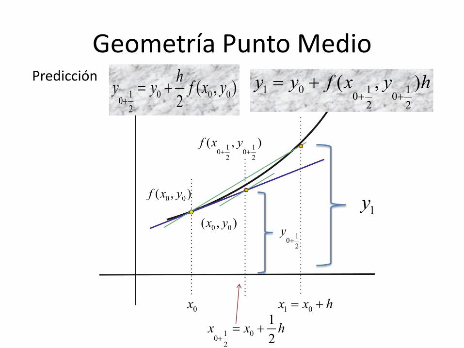
Geometría Punto Medio

0x

1 002

12

x x h+= +

1 0x x h= +

0 0( , )x y

0 0( , )f x y

1 10 02 2

( , )f x y+ +

102

y+

1 0 0 002

( , )2hy y f x y

+= +

Predicción

1y

1 0 1 10 02 2

( , )y y f x y h+ +

= +

Punto Medio

12

( , )2i i ii

hy y f x y+= +Predicción

1 1 12 2

( , )i i i iy y f x y h+

+ += +

Queremos aproximar numericamente soluciones de EDO’s de primer orden

Filosofía:

),( yxfdxdy

=

1

1

Valor nuevo valor viejo pendiente * (tamaño_paso)*

valor nuevo, valor viejo pendiente, tamaño de paso

i i

i i

y y hy y

h

ϕ

ϕ

+

+

= += +

¿Qué hemos hecho hasta el momento?

Runge Kuta

1

1

Valor nuevo valor viejo pendiente * (tamaño_paso)*

valor nuevo, valor viejo pendiente, tamaño de paso

i i

i i

y y hy y

h

ϕ

ϕ

+

+

= += +

Buscamos un método de la forma

De manera que la pendiente sea una pendiente ponderada sobre distintos puntos del intervalo [x(i),x(i+1)].

Runge Kuta de Cuarto Orden(Acto de fe)

1

1

Valor nuevo valor viejo pendiente * (tamaño_paso) *

valor nuevo, valor viejo pendiente, tamaño de paso

k k

k k

y y hy y

h

ϕ

ϕ

+

+

= += +

1nk

2nk

3nk4nk

nt 1n nt t h+ = +12nt h+

ny1ny +

( )1 1 2 3 41 * , 2 26k k n n n ny y h k k k kϕ ϕ+ = + = + + +

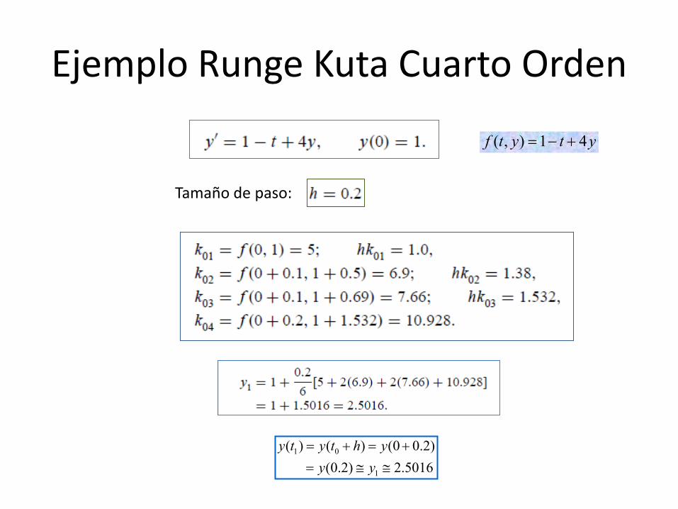
Ejemplo Runge Kuta Cuarto Orden

( , ) 1 4f t y t y= − +

1 0

1

( ) ( ) (0 0.2) (0.2) 2.5016y t y t h y

y y= + = +

= ≅ ≅

Tamaño de paso:

Otro ejemplo

Repitiendo el proceso

Tamaño de paso

Calculamos las cuatro

pendientes

(1) ?y =

Es necesario realizar dos “juegos“ de cálculos

Obtención de Runge Kuta de Segundo Orden1

1 1 2 2

i i

M M

y y ha k a k a k

ϕϕ

+ = += + + +

constantesia

1

2 1 11 1

3 2 21 1 22 2

1 1,1 1 1, 11 11

( , )( , )( , )

( , ... )

i i

i i

i i

M i M i M M M N

k f t yk f t p h y q k hk f t p h y q k h q k h

k f t p h y q k h q k h− − − − −

== + += + + +

= + + + +

es una pendiente ponderada de salidaϕ

23( ) ( ) '( ) ''( ) ( )

2Pero podemos calcular '( ) y ''( )

'( ) ( , ( ))( , ( )) ( , ( ))''( ) '( )

( , ( )) ( , ( )) ( , ( ))

i i i i

i i

i i i

i i i ii i

i i i ii i

hy t h y t y t h y t O h

y t y ty t f t y t

f t y t f t y ty t y tx y

f t y t f t y t f t y tx y

+ = + + +

=∂ ∂

= +∂ ∂

∂ ∂= + ⋅

∂ ∂

Aproximación de la solución por serie de Taylor de segundo orden alrededor de it t=

12

2

( ) ( )

( ) '( ) ''( )2

( , ( )) ( , ( )) = ( ) ( , ( )) ( , ( ))2

i i

i i i

i i i ii i i i i

y t y t hhy t y t h y t

f t y t f t y t hy t f t y t h f t y tx y

+ = +

≅ + +

∂ ∂+ + + ⋅ ∂ ∂

La aproximación obtenida está dada por

2

1

De esta forma,

( , ( )) ( , ( ))( )= ( ) ( , ( )) ( , ( ))2

i i i ii i i i i i

f t y t f t y t hy t y t f t y t h f t y tx y+

∂ ∂+ + + ⋅ ∂ ∂

( ) ( )( , ) ( , )( , ) ( , ) i i i ii i i i

f t y f t yf t H y K f t y H Kt y

∂ ∂+ + ≈ + +

∂ ∂

Aproximación por Serie de Taylor a primer orden de una función de dos variables

2kPara aproximar tomamos1 11 1 y H p h K q k h= =

De esta forma, obtenemos

[ ] [ ]2 1 11 1

1 11 1

( , )( , ) ( , ) ( , )

i i

i i i ii i

k f t p h y q k hf t y f t yf t y p h q k h

t y

= + +∂ ∂

= + ⋅ + ⋅∂ ∂

De esta forma

[ ] [ ]

[ ]

[ ]

1 1 2 2

1 2 1 11 1

1 2 2 1 2 11 1

1 2 2 1 2 11

( , ) ( , ) = ( , ) ( , )

( , ) ( , ) = ( , )

( , ) ( , ) = ( , ) ( , )

i i i ii i i i

i i i ii i

i i i ii i i i

a k a k

f t y f t ya f t y a f t y p h q k ht y

f t y f t ya a f t y h a p a q kt y

f t y f t ya a f t y h a p a q f t yt y

ϕ = +

∂ ∂+ + ⋅ + ⋅ ∂ ∂

∂ ∂+ + + ∂ ∂

∂ ∂+ + +

∂ ∂

En consecuencia,

[ ]

[ ]

1 1

1 2 2 1 2 11

21 2 2 1 2 11

( ) ( )

( , ) ( , ) = ( ) ( , ) ( , )

( , ) ( , ) = ( ) ( , ) ( , )

i i i i

i i i ii i i i i

i i i ii i i i i

y y t y h y t h

f t y f t yy t a a f t y h a p a q f t y ht y

f t y f t yy t a a f t y h a p a q f t y ht y

ϕ ϕ+ +≅ = + = +

∂ ∂+ + + + ∂ ∂

∂ ∂+ + + + ∂ ∂

[ ] 21 1 2 2 1 2 11

En resumen,

( , ) ( , )( ) ( ) ( , ) ( , )i i i ii i i i i i

f t y f t yy t y t a a f t y h a p a q f t y ht y+

∂ ∂= + + + + ∂ ∂

Hemos obtenido dos aproximaciones para , a saber:1( )iy t +

2

1( , ( )) ( , ( ))( )= ( ) ( , ( )) ( , ( ))

2i i i i

i i i i i if t y t f t y t hy t y t f t y t h f t y t

x y+

∂ ∂+ + + ⋅ ∂ ∂

[ ] 21 1 2 2 1 2 11

( , ) ( , )( ) ( ) ( , ) ( , )i i i ii i i i i i

f t y f t yy t y t a a f t y h a p a q f t y ht y+

∂ ∂= + + + + ∂ ∂

Igualando coeficientes

1 2 2 1 2 111 11, y 2 2

a a a p a q+ = = =

Es decir,

1 2 1 112 2

1 11 , y 2 2

a a p qa a

= − = =

Por lo que tenemos una infinidad de Métodos de Runge Kuta de orden 2, uno por cada valor que le demos al parámetro independiente 2a

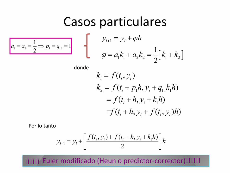
Casos particulares

1 2 1 111 12

a a p q= = ⇒ = =

[ ]1

1 1 2 2 1 212

i iy y h

a k a k k k

ϕ

ϕ

+ = +

= + = +

1

2 1 11 1

1

( , )( , )

( , ) = ( , ( , ) )

i i

i i

i i

i i i i

k f t yk f t p h y q k h

f t h y k hf t h y f t y h

== + += + +

+ +

donde

Por lo tanto

11

( , ) ( , )2

i i i ii i

f t y f t h y k hy y h+

+ + + = +

¡¡¡¡¡¡¡Euler modificado (Heun o predictor-corrector)!!!!!!

Casos particulares1 2 1 11

10, 12

a a p q= = ⇒ = = 1

1 1 2 2 2

i iy y ha k a k k

ϕϕ

+ = += + =

2 1 11 1( , )1 1 ( , ( , ) )2 2

i i

i i i i

k f t p h y q k h

f t h y f t y h

= + +

= + +

donde

Por lo tanto1 1

1 1

( , ) = ( , )

i i i i

i i i

y y f t h y k h hy f t y k h h

+

+

= + + ++ +

1 1

1 1

( , ) = ( , )

i i i i

i i i

y y f t h y k h hy f t y k h h

+

+

= + + ++ +

1 1 ( , )i i i i iy y k h y f t y h+ = + = +

1 1

1 1

( , ) = ( , )

i i i i

i i i

y y f t h y k h hy f t y h

+

+ +

= + + ++

Se conoce como Euler hacia atrás

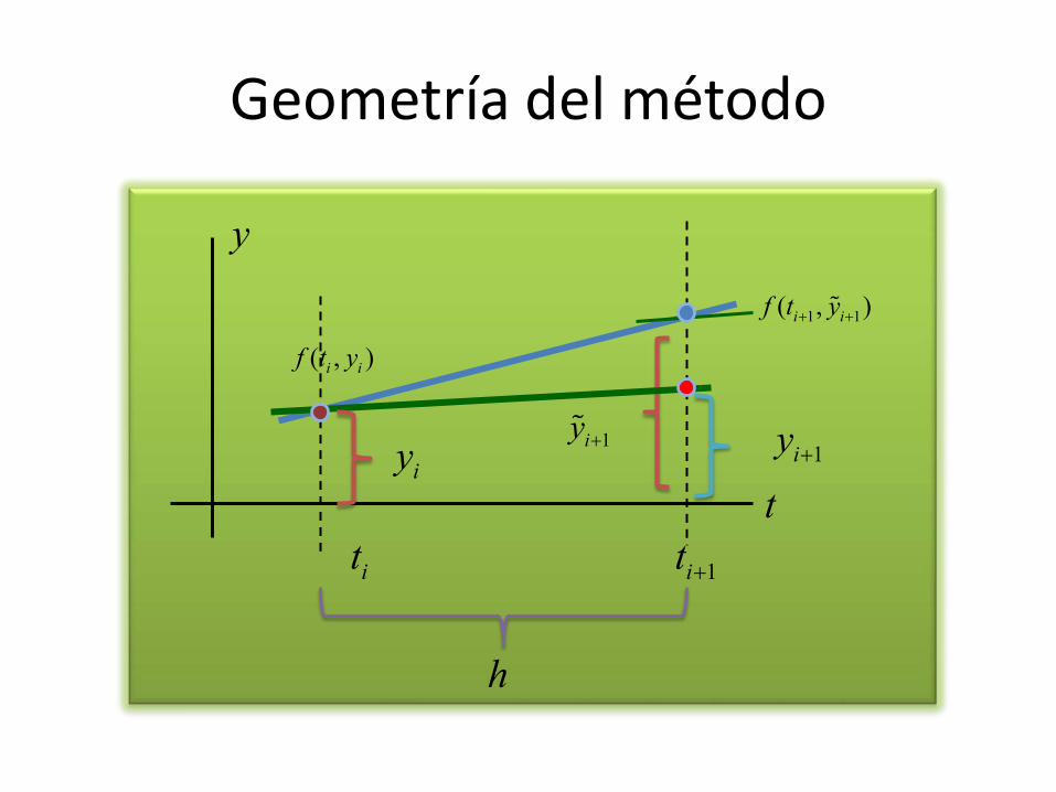
1iy +1iy +

iy

( , )i if t y

it 1it +

1 1( , )i if t y+ +

t

y

Geometría del método

h