Automatic change detection in multiple pigmented skin lesions
219
AUTOMATIC CHANGE DETECTION IN MULTIPLE PIGMENTED SKIN LESIONS Konstantin Korotkov Dipòsit legal: Gi. 1344-2014 http://hdl.handle.net/10803/260162 ADVERTIMENT. L'accés als continguts d'aquesta tesi doctoral i la seva utilització ha de respectar els drets de la persona autora. Pot ser utilitzada per a consulta o estudi personal, així com en activitats o materials d'investigació i docència en els termes establerts a l'art. 32 del Text Refós de la Llei de Propietat Intel·lectual (RDL 1/1996). Per altres utilitzacions es requereix l'autorització prèvia i expressa de la persona autora. En qualsevol cas, en la utilització dels seus continguts caldrà indicar de forma clara el nom i cognoms de la persona autora i el títol de la tesi doctoral. No s'autoritza la seva reproducció o altres formes d'explotació efectuades amb finalitats de lucre ni la seva comunicació pública des d'un lloc aliè al servei TDX. Tampoc s'autoritza la presentació del seu contingut en una finestra o marc aliè a TDX (framing). Aquesta reserva de drets afecta tant als continguts de la tesi com als seus resums i índexs. ADVERTENCIA. El acceso a los contenidos de esta tesis doctoral y su utilización debe respetar los derechos de la persona autora. Puede ser utilizada para consulta o estudio personal, así como en actividades o materiales de investigación y docencia en los términos establecidos en el art. 32 del Texto Refundido de la Ley de Propiedad Intelectual (RDL 1/1996). Para otros usos se requiere la autorización previa y expresa de la persona autora. En cualquier caso, en la utilización de sus contenidos se deberá indicar de forma clara el nombre y apellidos de la persona autora y el título de la tesis doctoral. No se autoriza su reproducción u otras formas de explotación efectuadas con fines lucrativos ni su comunicación pública desde un sitio ajeno al servicio TDR. Tampoco se autoriza la presentación de su contenido en una ventana o marco ajeno a TDR (framing). Esta reserva de derechos afecta tanto al contenido de la tesis como a sus resúmenes e índices. WARNING. Access to the contents of this doctoral thesis and its use must respect the rights of the author. It can be used for reference or private study, as well as research and learning activities or materials in the terms established by the 32nd article of the Spanish Consolidated Copyright Act (RDL 1/1996). Express and previous authorization of the author is required for any other uses. In any case, when using its content, full name of the author and title of the thesis must be clearly indicated. Reproduction or other forms of for profit use or public communication from outside TDX service is not allowed. Presentation of its content in a window or frame external to TDX (framing) is not authorized either. These rights affect both the content of the thesis and its abstracts and indexes.
Transcript of Automatic change detection in multiple pigmented skin lesions
AUTOMATIC CHANGE DETECTION IN MULTIPLE PIGMENTED SKIN LESIONS
Konstantin Korotkov
Dipòsit legal: Gi. 1344-2014 http://hdl.handle.net/10803/260162
ADVERTIMENT. L'accés als continguts d'aquesta tesi doctoral i la seva utilització ha de respectar els drets de la persona autora. Pot ser utilitzada per a consulta o estudi personal, així com en activitats o materials d'investigació i docència en els termes establerts a l'art. 32 del Text Refós de la Llei de Propietat Intel·lectual (RDL 1/1996). Per altres utilitzacions es requereix l'autorització prèvia i expressa de la persona autora. En qualsevol cas, en la utilització dels seus continguts caldrà indicar de forma clara el nom i cognoms de la persona autora i el títol de la tesi doctoral. No s'autoritza la seva reproducció o altres formes d'explotació efectuades amb finalitats de lucre ni la seva comunicació pública des d'un lloc aliè al servei TDX. Tampoc s'autoritza la presentació del seu contingut en una finestra o marc aliè a TDX (framing). Aquesta reserva de drets afecta tant als continguts de la tesi com als seus resums i índexs. ADVERTENCIA. El acceso a los contenidos de esta tesis doctoral y su utilización debe respetar los derechos de la persona autora. Puede ser utilizada para consulta o estudio personal, así como en actividades o materiales de investigación y docencia en los términos establecidos en el art. 32 del Texto Refundido de la Ley de Propiedad Intelectual (RDL 1/1996). Para otros usos se requiere la autorización previa y expresa de la persona autora. En cualquier caso, en la utilización de sus contenidos se deberá indicar de forma clara el nombre y apellidos de la persona autora y el título de la tesis doctoral. No se autoriza su reproducción u otras formas de explotación efectuadas con fines lucrativos ni su comunicación pública desde un sitio ajeno al servicio TDR. Tampoco se autoriza la presentación de su contenido en una ventana o marco ajeno a TDR (framing). Esta reserva de derechos afecta tanto al contenido de la tesis como a sus resúmenes e índices. WARNING. Access to the contents of this doctoral thesis and its use must respect the rights of the author. It can be used for reference or private study, as well as research and learning activities or materials in the terms established by the 32nd article of the Spanish Consolidated Copyright Act (RDL 1/1996). Express and previous authorization of the author is required for any other uses. In any case, when using its content, full name of the author and title of the thesis must be clearly indicated. Reproduction or other forms of for profit use or public communication from outside TDX service is not allowed. Presentation of its content in a window or frame external to TDX (framing) is not authorized either. These rights affect both the content of the thesis and its abstracts and indexes.
PhD Thesis
Automatic Change Detection in
Multiple Pigmented Skin Lesions
Konstantin Korotkov
2014

PhD Thesis
Automatic Change Detection in
Multiple Pigmented Skin Lesions
Konstantin Korotkov
2014
DOCTORAL PROGRAM IN TECHNOLOGY
Supervised by: Dr. Rafael Garcıa
Work submitted to the University of Girona in partial fulfillment of the requirements
for the degree of Doctor of Philosophy


Ïîñâÿùàåòñÿ ìîèì ðîäèòåëÿì
Dedicated to my parents


Acknowledgements
I believe that courage and inspiration are the essential ingredients that make up
and sustain any endeavor. I am lucky that during my doctoral studies I have always
had a source of both, and for that, I am sincerely grateful to my supervisor, Rafael
Garcıa. Without his brilliant ideas and continuous support, this work would simply
not be possible. Nor would it be possible without my family that has always been there
for me despite the overwhelming distances between us. Their love and encouragement
helped me immensely in the completion of this thesis. My most loving thanks to my
parents, Natalya and Evgeniy, brother Kirill, grandma Elizaveta, aunt Anna and uncle
Alexander, cousins, Nikolay and Kseniya, my great grandmother Galina and granduncle
Alexander.
My special thanks go to my friends many of whom are fellow PhD students and
know first-hand what it takes to be one. They were there to help me out whenever
I needed it the most: Kenneth, Victor, Isaac, Guillaume, Mojdeh, Habib, Sharad,
Chrissy, Chee Sing, Shihav, Sonia, Jan, and Andrey.
Also, I would like to thank my colleagues: Nuno, Tudor and Laszlo, for their time
and invaluable suggestions; Josep, Ricard P. and Ricard C., for taking the trouble to
help me with all my technical problems; and Joseta, Mireia, and Montse, for keeping
my back in the ruthless world of paperwork. My gratitude, as well, to the anonymous
reviewers and the members of the defense panel for evaluating my work. Besides, this
thesis largely owes its completion to the AGAUR FI-DGR 2011 grant provided by the
Autonomous Government of Catalonia. I am grateful and honored to be among its
holders.
Last but never least, I wish to thank my fiancee, and soon to be wife, Amanda,
for standing beside me throughout my PhD. Her unwavering faith in me, even at the
times when I could not share it, her patience and love encouraged me not to give up
and accomplish what I had undertaken.
v


Publications
This thesis resulted in the publication of a comprehensive review article:
K. Korotkov and R. Garcıa, “Computerized analysis of pigmented skin lesions: a
review,” Artificial Intelligence in Medicine, 2012, 56, 69–90.
Also, an article titled “Design, Construction, and Testing of a New Total Body Skin
Scanning System” is currently under review in the IEEE Transactions of Medical Imag-
ing journal.
vii

viii

Abbreviations
ANN Artificial Neural Networks
CAD Computer-Aided Diagnosis
CBIR Content-Based Image Retrieval
CCD Charge-Coupled Device
CDS Clinical Diagnosis Support
CIELUV Commission Internationale de l’Eclairage 1976 (L∗ u∗ v∗) color space
DA Discriminant Analysis
DOF Depth of Field
DTEA Dermatologist-like Tumour Extraction Algorithm
ELM Epiluminiscence Microscopy
GVF Gradient Vector Flow
HSV Hue Saturation Intensity (color space)
JPEG Joint Photographic Experts Group
KL-PLS Kernel Logistic Partial Least Squares
KLT Karhunen-Loeve Transform
kNN k-Nearest Neighbors
ix

ABBREVIATIONS
LED Light-Emitting Diode
MSER Maximally Stable Extremal Regions
NCC Normalized Cross-Correlation
PCA Principal Component Analysis
PDE Partial Differential Equations
PSL Pigmented Skin Lesion
RANSAC RAndom SAmple Consensus
RGB Red Green Blue (color space)
ROI Region of Interest
SIFT Scale-Invariant Feature Transform
SRM Statistical Region Merging
SVM Support Vector Machines
TBSE Total Body Skin Examination
TBSI Total Body Skin Imaging
UV Ultraviolet radiation
WBP Whole Body Photography
x

List of Figures
1.1 Anatomy of the skin . . . . . . . . . . . . . . . . . . . . . . . . . . . . . 2
1.2 Clinical and dermoscopic images of benign PSLs . . . . . . . . . . . . . 4
1.3 Clinical and dermoscopic images of malignant melanomas . . . . . . . . 6
1.4 Standardized poses for TBSI . . . . . . . . . . . . . . . . . . . . . . . . 9
1.5 Samples of commercially available dermoscopes . . . . . . . . . . . . . . 10
1.6 Two dermoscopy images of a PSL acquired with a difference of one year 15
2.1 Literature categorization tree . . . . . . . . . . . . . . . . . . . . . . . . 18
3.1 Exterior view of the scanner: the acquisition compartment . . . . . . . . 47
3.2 Exterior view of the scanner: the equipment compartment . . . . . . . . 48
3.3 The camera setup and patient poses for image acquisition . . . . . . . . 52
3.4 Schematic views of the turntable steps . . . . . . . . . . . . . . . . . . . 53
3.5 Schematic representation of the coordinate systems in the scanner . . . 59
3.6 Marker encoding using the colors of the surrounding squares . . . . . . . 61
3.7 The abacus encoding scheme for 4 colors . . . . . . . . . . . . . . . . . . 62
3.8 Images of the calibration pattern . . . . . . . . . . . . . . . . . . . . . . 63
3.9 Neighbor corners selection in the pattern . . . . . . . . . . . . . . . . . . 66
3.10 Sample images demonstrating imaging subsystem limitations . . . . . . 68
3.11 The limits of the patient area in the acquisition chamber . . . . . . . . . 68
4.1 The pipeline for intra-exploration mole mapping . . . . . . . . . . . . . 72
4.2 Image projection of a lesion’s normal vector . . . . . . . . . . . . . . . . 79
4.3 Schematics of possible scenarios during mole set creation . . . . . . . . . 81
4.4 Failed homography computation using SIFT features . . . . . . . . . . . 82
4.5 Single representation of two lesions . . . . . . . . . . . . . . . . . . . . . 83
4.6 Best camera/view selection during mole set merging . . . . . . . . . . . 86
4.7 Mole comparison scenarios . . . . . . . . . . . . . . . . . . . . . . . . . . 88
4.8 The lesion matching condition during the mole set merging procedure . 89
xi
LIST OF FIGURES
4.9 Mole match propagation: possible bridge exception scenarios . . . . . . 90
4.10 The pipeline for detecting new and evolving lesions . . . . . . . . . . . . 92
4.11 An example of non-coinciding views of the same mole in 2 explorations . 93
4.12 Scenarios for the view selection in the target exploration . . . . . . . . . 95
5.1 Skin (foreground) detection . . . . . . . . . . . . . . . . . . . . . . . . . 104
5.2 Image preprocessing for mole detection . . . . . . . . . . . . . . . . . . . 106
5.3 Mole detection using MSER . . . . . . . . . . . . . . . . . . . . . . . . . 108
5.4 SIFT feature matches in stereo images . . . . . . . . . . . . . . . . . . . 110
5.5 Mole correspondences in stereo pairs . . . . . . . . . . . . . . . . . . . . 112
5.6 Evaluation of PSL stereo triangulation . . . . . . . . . . . . . . . . . . . 114
5.7 Mole sets computed at three different turntable positions . . . . . . . . 115
5.8 Overlapping mole sets . . . . . . . . . . . . . . . . . . . . . . . . . . . . 116
5.9 Mole matching at different turntable positions . . . . . . . . . . . . . . . 118
5.10 Unsuccessful matching of moles at remote turntable positions . . . . . . 119
5.11 Mole set match propagation . . . . . . . . . . . . . . . . . . . . . . . . . 120
5.12 Examples of outliers in the mole map . . . . . . . . . . . . . . . . . . . . 121
5.13 A complete mole map of a reference patient . . . . . . . . . . . . . . . . 122
5.14 Clinical and dermoscopy images of relevant lesions of a patient . . . . . 125
5.15 Inter-exploration lesion matching . . . . . . . . . . . . . . . . . . . . . . 127
5.16 Change detection in PSLs . . . . . . . . . . . . . . . . . . . . . . . . . . 129
A.1 Sample image of binarization using different intensity thresholds . . . . 138
A.2 Example of a MSER detection with different parameters . . . . . . . . . 139
A.3 Point correspondence and epipolar geometry . . . . . . . . . . . . . . . . 141
A.4 Image scale-space representation . . . . . . . . . . . . . . . . . . . . . . 144
A.5 The scale-space pyramid used in SIFT . . . . . . . . . . . . . . . . . . . 145
A.6 Extrema detection in the difference-of-Gaussian images . . . . . . . . . . 146
A.7 Creation of a SIFT keypoint descriptor . . . . . . . . . . . . . . . . . . . 149
A.8 Sample SIFT feature detection . . . . . . . . . . . . . . . . . . . . . . . 151
A.9 Triangulation of a 3D point using its projections in stereo images . . . . 153
A.10 Line parameterization . . . . . . . . . . . . . . . . . . . . . . . . . . . . 154
xii

List of Tables
1.1 Methods for the diagnosis of melanoma clinically and by dermoscopy. . . 12
1.2 Confusing acronyms of methods for melanoma diagnosis . . . . . . . . . 13
2.1 PSL image preprocessing operations . . . . . . . . . . . . . . . . . . . . 20
2.2 Feature extraction for pattern analysis . . . . . . . . . . . . . . . . . . . 27
2.3 Dermoscopic features of PSLs . . . . . . . . . . . . . . . . . . . . . . . . 28
2.4 Clinical features of PSLs . . . . . . . . . . . . . . . . . . . . . . . . . . . 30
2.5 Classification methods in computerized analysis of PSL images . . . . . 36
2.6 Proprietary CAD software and dermoscopy instruments . . . . . . . . . 38
3.1 The intrinsic parameters of the cameras . . . . . . . . . . . . . . . . . . 57
4.1 Summary of the algorithm parameters . . . . . . . . . . . . . . . . . . . 100
xiii

LIST OF TABLES
xiv

List of Algorithms
1 Primary steps for visual marker identification . . . . . . . . . . . . . . . . 64
2 Image foreground (skin) detection . . . . . . . . . . . . . . . . . . . . . . 74
3 Image preprocessing for mole detection . . . . . . . . . . . . . . . . . . . 75
4 Mole matching in a stereo pair . . . . . . . . . . . . . . . . . . . . . . . . 77
5 Resolving a bridge exception during mole match propagation . . . . . . . 91
6 PSL change detection . . . . . . . . . . . . . . . . . . . . . . . . . . . . . 98
7 The RANSAC robust estimation algorithm. . . . . . . . . . . . . . . . . . 151
8 Adaptive algorithm for determining the number of RANSAC samples . . 152
xv

LIST OF ALGORITHMS
xvi
Contents
Abbreviations ix
List of Figures xi
List of Tables xiii
List of Algorithms xv
Abstract xxv
1 Introduction 1
1.1 The human skin . . . . . . . . . . . . . . . . . . . . . . . . . . . . . . . 1
1.2 Pigmented skin lesions . . . . . . . . . . . . . . . . . . . . . . . . . . . . 3
1.3 Malignant melanoma . . . . . . . . . . . . . . . . . . . . . . . . . . . . . 5
1.4 Melanoma screening . . . . . . . . . . . . . . . . . . . . . . . . . . . . . 7
1.4.1 Imaging techniques . . . . . . . . . . . . . . . . . . . . . . . . . . 7
1.4.1.1 Clinical photography . . . . . . . . . . . . . . . . . . . 8
1.4.1.2 Dermoscopy . . . . . . . . . . . . . . . . . . . . . . . . 9
1.4.1.3 Baseline images . . . . . . . . . . . . . . . . . . . . . . 10
1.4.2 Melanoma diagnosis methods . . . . . . . . . . . . . . . . . . . . 11
1.4.3 Automated diagnosis of melanoma . . . . . . . . . . . . . . . . . 12
1.4.3.1 Clinical impact . . . . . . . . . . . . . . . . . . . . . . . 13
1.5 Research motivation . . . . . . . . . . . . . . . . . . . . . . . . . . . . . 14
1.6 Thesis outline . . . . . . . . . . . . . . . . . . . . . . . . . . . . . . . . . 16
2 Computerized analysis of PSLs: a literature review 17
2.1 Single lesion analysis . . . . . . . . . . . . . . . . . . . . . . . . . . . . . 19
2.1.1 Image preprocessing . . . . . . . . . . . . . . . . . . . . . . . . . 20
2.1.2 Lesion border detection . . . . . . . . . . . . . . . . . . . . . . . 21
2.1.2.1 PSL border detection methodology . . . . . . . . . . . . 22
2.1.2.2 Comparison of segmentation algorithms . . . . . . . . . 24
2.1.3 Feature extraction . . . . . . . . . . . . . . . . . . . . . . . . . . 25
2.1.4 Registration and change detection . . . . . . . . . . . . . . . . . 32
xvii

CONTENTS
2.1.4.1 Change detection . . . . . . . . . . . . . . . . . . . . . 32
2.1.4.2 Registration . . . . . . . . . . . . . . . . . . . . . . . . 33
2.1.5 Lesion classification . . . . . . . . . . . . . . . . . . . . . . . . . 34
2.1.6 CAD systems . . . . . . . . . . . . . . . . . . . . . . . . . . . . . 37
2.1.7 3D lesion analysis . . . . . . . . . . . . . . . . . . . . . . . . . . 40
2.2 Multiple lesion analysis . . . . . . . . . . . . . . . . . . . . . . . . . . . 40
2.2.1 Lesion localization . . . . . . . . . . . . . . . . . . . . . . . . . . 41
2.2.2 Lesion registration . . . . . . . . . . . . . . . . . . . . . . . . . . 41
2.3 Conclusion . . . . . . . . . . . . . . . . . . . . . . . . . . . . . . . . . . 42
3 A total body skin scanner 45
3.1 Hardware design . . . . . . . . . . . . . . . . . . . . . . . . . . . . . . . 46
3.1.1 The imaging subsystem . . . . . . . . . . . . . . . . . . . . . . . 49
3.1.2 The lighting subsystem . . . . . . . . . . . . . . . . . . . . . . . 50
3.2 The scanning procedure . . . . . . . . . . . . . . . . . . . . . . . . . . . 51
3.3 Camera calibration . . . . . . . . . . . . . . . . . . . . . . . . . . . . . . 53
3.3.1 The intrinsic calibration . . . . . . . . . . . . . . . . . . . . . . . 53
3.3.2 The extrinsic calibration . . . . . . . . . . . . . . . . . . . . . . . 58
3.3.2.1 The calibration board . . . . . . . . . . . . . . . . . . . 59
3.3.2.2 Visual marker recognition . . . . . . . . . . . . . . . . . 63
3.4 Prototype restrictions . . . . . . . . . . . . . . . . . . . . . . . . . . . . 67
3.5 Conclusions . . . . . . . . . . . . . . . . . . . . . . . . . . . . . . . . . . 69
4 Automatic PSL change detection 71
4.1 Intra-exploration mole mapping . . . . . . . . . . . . . . . . . . . . . . . 71
4.1.1 Mole detection . . . . . . . . . . . . . . . . . . . . . . . . . . . . 72
4.1.1.1 Foreground (skin) detection . . . . . . . . . . . . . . . . 72
4.1.1.2 Image preprocessing . . . . . . . . . . . . . . . . . . . . 73
4.1.2 Stereo-pair processing . . . . . . . . . . . . . . . . . . . . . . . . 75
4.1.2.1 Mole matching . . . . . . . . . . . . . . . . . . . . . . . 76
4.1.2.2 Mole triangulation . . . . . . . . . . . . . . . . . . . . . 78
4.1.3 Mole set creation . . . . . . . . . . . . . . . . . . . . . . . . . . . 79
4.1.3.1 Multiple representations of one lesion . . . . . . . . . . 80
4.1.3.2 Single representation of multiple lesions . . . . . . . . . 82
4.1.4 Mole set merging . . . . . . . . . . . . . . . . . . . . . . . . . . . 83
4.1.4.1 Matching moles across mole sets . . . . . . . . . . . . . 84
xviii

CONTENTS
4.1.4.2 Mole match propagation . . . . . . . . . . . . . . . . . 89
4.2 Inter-exploration operations . . . . . . . . . . . . . . . . . . . . . . . . . 91
4.2.1 Mole matching . . . . . . . . . . . . . . . . . . . . . . . . . . . . 92
4.2.2 Change detection . . . . . . . . . . . . . . . . . . . . . . . . . . . 97
4.3 Conclusion . . . . . . . . . . . . . . . . . . . . . . . . . . . . . . . . . . 98
5 Results and discussion 103
5.1 Intra-exploration operations . . . . . . . . . . . . . . . . . . . . . . . . . 103
5.1.1 Skin detection . . . . . . . . . . . . . . . . . . . . . . . . . . . . 103
5.1.2 Image preprocessing . . . . . . . . . . . . . . . . . . . . . . . . . 105
5.1.3 Mole detection . . . . . . . . . . . . . . . . . . . . . . . . . . . . 107
5.1.4 Mole matching in stereo pairs . . . . . . . . . . . . . . . . . . . . 109
5.1.5 PSL triangulation and mole set creation . . . . . . . . . . . . . . 113
5.1.6 Mole set merging . . . . . . . . . . . . . . . . . . . . . . . . . . . 117
5.2 Mole map validation . . . . . . . . . . . . . . . . . . . . . . . . . . . . . 121
5.2.1 The ground truth problem . . . . . . . . . . . . . . . . . . . . . . 121
5.2.2 Preliminary evaluation . . . . . . . . . . . . . . . . . . . . . . . . 123
5.3 Inter-exploration operations . . . . . . . . . . . . . . . . . . . . . . . . . 126
5.3.1 Lesion matching . . . . . . . . . . . . . . . . . . . . . . . . . . . 126
5.3.2 Change detection . . . . . . . . . . . . . . . . . . . . . . . . . . . 128
6 Conclusions 131
6.1 Summary of the thesis . . . . . . . . . . . . . . . . . . . . . . . . . . . . 132
6.2 Contributions . . . . . . . . . . . . . . . . . . . . . . . . . . . . . . . . . 133
6.3 Limitations . . . . . . . . . . . . . . . . . . . . . . . . . . . . . . . . . . 134
6.4 Further work . . . . . . . . . . . . . . . . . . . . . . . . . . . . . . . . . 134
A Methodology 137
A.1 Maximally Stable Extremal Regions . . . . . . . . . . . . . . . . . . . . 137
A.2 Epipolar geometry . . . . . . . . . . . . . . . . . . . . . . . . . . . . . . 140
A.3 Scale-Invariant Feature Transform . . . . . . . . . . . . . . . . . . . . . 142
A.4 The RANSAC algorithm . . . . . . . . . . . . . . . . . . . . . . . . . . . 150
A.5 Triangulation . . . . . . . . . . . . . . . . . . . . . . . . . . . . . . . . . 153
References 157
xix

CONTENTS
xx
Resum
El melanoma maligne es el mes rar i mortal de tots els cancers de pell, causant tres
vegades mes morts que el conjunt de totes les altres malalties malignes de la pell. Afor-
tunadament, en les primeres etapes, es completament curable, fent de les exploracions
de pell a nivell de cos complert (TBSE, de l’angles Total Body Skin Examination) un
proces fonamental per a molts pacients. Durant el TBSE, els dermatolegs busquen els
signes tıpics de melanoma en les lesions pigmentades de la pell (PSL, Pigmented Skin
Lesions), aixı com PSLs sotmesos als rapids canvis caracterıstics del cancer. Conjunta-
ment amb la fotografia de referencia clınica i dermatoscopica, el calcul de TBSE pot ser
molt tedios i lent, especialment per a pacients amb un gran nombre de lesions. A mes
a mes, establir correspondencies correctes entre el cos i les imatges, i entre les diferents
imatges, per a cadascuna de les lesions, pot esser d’extrema dificultat.
Malgrat els avencos en les tecniques d’escaneig cutani, les eines per a realitzar
TBSEs de forma automatica no han rebut massa atencio. Aquest fet es posa de relleu en
la nostra revisio de la literatura, que cobreix l’area de l’analisi per computador d’imatges
de PSL. En aquesta revisio, es resumeixen varies aproximacions per a la implementacio
del diagnostic assistit per ordinador, comentant-ne els seus components principals. En
particular, es proposa una classificacio ampliada de descriptors de caracterıstiques PSL,
associant-los amb metodes especıfics pel diagnostic de melanoma, dividint-los entre
imatge clınica i dermatoscopica.
Amb l’objectiu de l’automatitzacio de TBSEs, hem dissenyat i construıt un escaner
corporal de cobertura total per adquirir imatges de la superfıcie de la pell utilitzant llum
amb polaritzacio creuada. Equipat amb 21 cameres d’alta resolucio de baix cost i una
plataforma giratoria, aquest escaner adquireix automaticament un conjunt d’imatges
amb solapament, que cobreix el 85–90% de la superfıcie de la pell del pacient. La
calibracio extrınseca del sistema es du a terme utilitzant una sola imatge de cada camera
i un patro de calibratge amb un codi de colors dissenyat especıficament. A mes, hem
desenvolupat un algoritme pel mapeig automatic de les PSLs i l’estimacio dels canvis
entre exploracions. Els mapes produıts relacionen les imatges de les lesions individuals
amb la seva ubicacio en el cos del pacient, resolent el problema de correspondencia
del cos a la imatge i d’imatge a imatge en TBSEs. Actualment, l’escaner es limita a
pacients amb escas pel corporal. Per a un examen complet de la pell, on el cuir cabellut,
els palmells de les mans, les plantes dels peus i les parts interiors dels bracos han de
ser fotografiats manualment.
Els tests inicials de l’escaner mostren que aquest pot esser utilitzat satisfactoriament
xxi

pel mapeig automatic i el control de canvis temporal de multiples lesions: els PSLs
importants per a realitzar-ne el seguiment han estat mapejats successivament en les
diverses exploracions. D’altra banda, durant la comparacio d’imatges, totes les lesions
amb canvis artificials introduıts han estat correctament identificades com “evoluciona-
des”. Per tal de desenvolupar estudis clınics mes amplis, amb diferents tipus de pell,
l’escaner s’ha instal.lat a la Unitat de Melanoma de l’Hospital Clınic de Barcelona.
xxii
Resumen
El melanoma maligno es el mas raro y mortal de todos los canceres de piel, cau-
sando tres veces mas muertes que el conjunto de todas las enfermedades malignas de la
piel. Afortunadamente, en las etapas tempranas, es completamente curable, haciendo
que el examen de piel de cuerpo completo (del ingles Total Body Skin Examination,
TBSE) sea un procedimiento fundamental para muchos pacientes. Durante el TBSE,
los dermatologos buscan los signos tıpicos de melanoma en las lesiones pigmentadas de
la piel (Pigmented Skin Lesions, PSLs), ası como PSLs sometidas a los rapidos cambios
caracterısticos del cancer. Junto a la fotografıa de referencia clınica y dermatoscopica,
un TBSE puede ser muy tedioso y lento, especialmente para los pacientes con gran
numero de lesiones. Ademas, establecer correspondencias correctas entre las lesiones
en el cuerpo y las imagenes, o en diferentes imagenes, puede ser extremadamente difıcil.
A pesar de los avances en las tecnicas del escaneo corporal, las herramientas para re-
alizar TBSEs de forma automatica no han recibido la debida atencion. Este hecho queda
patente en nuestra revision bibliografica que cubre el analisis de imagenes por computa-
dor de PSLs. En esta revision, se resumen varias estrategias para la implementacion
del diagnostico asistido por ordenador, comentando sus componentes principales. En
concreto, se propone una clasificacion ampliada de descriptores de caracterısticas PSL,
asociandolos con metodos especıficos para el diagnostico del melanoma, y dividiendolos
entre imagen clınica y dermatoscopica.
Con el objetivo de la automatizacion de TBSEs, hemos disenado y construido un
escaner corporal de cobertura total para adquirir imagenes de la superficie de la piel
utilizando luz con polarizacion cruzada. Equipado con 21 camaras de alta resolucion
de bajo coste y una plataforma giratoria, este escaner adquiere automaticamente un
conjunto de imagenes con solapamiento, que cubre el 85–90% de la superficie de la piel
del paciente. La calibracion extrınseca del sistema se lleva a cabo utilizando una sola
imagen de cada camara y un patron de calibracion con un codigo de colores disenado
especıficamente. Ademas, hemos desarrollado un algoritmo por mapeo automatico de
las PSLs y la estimacion de los cambios entre exploraciones. Los mapas producidos
relacionan las imagenes de las lesiones individuales con su ubicacion en el cuerpo del
paciente, resolviendo el problema de correspondencia cuerpo-imagen e imagen-imagen
de las lesiones en TBSEs. Actualmente, el escaner se limita a pacientes con escaso
vello corporal. Asimismo, para un examen completo de la piel, el cuero cabelludo, las
palmas de las manos, las plantas de los pies y las partes interiores de los brazos deben
ser fotografiadas manualmente.
xxiii

Las pruebas iniciales del escaner muestran que este puede ser utilizado satisfac-
toriamente para el mapeo automatico y el control de cambios temporal de multiples
lesiones: los PSLs importantes para realizar el seguimiento eran mapeados sucesiva-
mente en varias exploraciones. Por otra parte, durante la comparacion de imagenes,
todas las lesiones en las que se han introducido cambios artificiales, han sido correc-
tamente identificadas como “evolucionadas”. Para desarrollar estudios clınicos mas
amplios con diferentes tipos de piel, el escaner se ha instalado en la Unidad de Mela-
noma del Hospital Clınic de Barcelona.
xxiv
Abstract
Malignant melanoma is the rarest and deadliest of skin cancers causing three times
more deaths than all other skin-related malignancies combined. Fortunately, in its
early stages, it is completely curable, making a total body skin examination (TBSE) a
fundamental procedure for many patients. During TBSE, dermatologists look for pig-
mented skin lesions (PSLs) exhibiting typical melanoma signs as well as PSLs undergo-
ing the rapid changes characteristic of cancer. Accompanied by clinical and dermoscopic
baseline photography, a TBSE can be very tedious and time-consuming, especially for
patients with numerous lesions. In addition, establishing correct body-to-image and
image-to-image lesion correspondences can be extremely difficult.
Despite the advances in body scanning techniques, automated assistance tools for
TBSEs have not received due attention. This fact is emphasized in our literature
review covering the area of computerized analysis of PSL images. In this review, we
summarize various approaches for implementing PSL computer-aided diagnosis systems
and discuss their standard workflow components. In particular, we propose an extended
categorization of PSL feature descriptors, associating them with specific methods for
diagnosing melanoma, and separating clinical and dermoscopic images.
Aiming at the automation of TBSEs, we have designed and built a total body
scanner to acquire skin surface images using cross-polarized light. Equipped with 21
low-cost high-resolution cameras and a turntable, this scanner automatically acquires
a set of overlapping images, covering 85–90% of the patient’s skin surface. A one-
shot extrinsic calibration of all the cameras is carried out using a specifically designed
color-coded calibration pattern. Furthermore, we have developed an algorithm for
the automated mapping of PSLs and their change estimation between explorations.
The maps produced relate images of individual lesions with their locations on the
patient’s body, solving the body-to-image and image-to-image correspondence problem
in TBSEs. Currently, the scanner is limited to patients with sparse body hair and,
for a complete skin examination, the scalp, palms, soles and inner arms should be
photographed manually.
The initial tests of the scanner showed that it can be successfully applied for auto-
mated mapping and temporal monitoring of multiple lesions: PSLs relevant for follow-
up were repeatedly mapped in several explorations. Moreover, during the baseline
image comparison, all lesions with artificially induced changes were correctly identified
as “evolved”. In order to perform a wider clinical trial with a diverse skin image set, the
scanner has been installed in the Melanoma Unit at the Clinic Hospital of Barcelona.
xxv

xxvi
Moles are blemishes—not “beauty spots”.
Stanford Cade, “Malignant Melanoma” [2]
Chapter 1
Introduction
The skin is the largest organ in the human body and an excellent protection from
the aggressions of the environment. It keeps us safe from infections, water loss and
ultraviolet radiation (UV). However, if care is not taken, after years of faithful service,
the protector itself can turn into a treacherous and merciless foe: the skin can become
a source of a deadly cancer. Fortunately, this does not happen without warning: the
skin usually exhibits signs which can help detect this dangerous metamorphosis. These
signs may differ according to the type of malignancy and can sometimes be hard to
perceive. Thus, one of the key indicators of malignant melanoma—the deadliest skin
cancer—are melanocytic nevi, also known as moles or pigmented skin lesions (PSLs).
The occurrence of nevi, their appearance and especially their evolution can indicate a
developing or progressing malignancy.
To understand the nature of malignant tumors of the skin better and see how
computer vision can help in their treatment, it is essential to know more about the
clinical aspects of this problem. In this chapter, we offer a brief introduction into the
main dermatological concepts related to melanoma of the skin.
1.1 The human skin
The skin consists of two principal layers: the epidermis and the dermis (see Fig. 1.1).
The dermis is made of collagen (a type of protein) and elastic fibers. It contains two
sub-layers: the papillary dermis (thin layer) and the reticular dermis (thick layer).
While the former serves as a “glue” that holds the epidermis and the dermis together,
the latter contains blood and lymph vessels, nerve endings, sweat glands and hair
follicles. It provides energy and nutrition to the epidermis and plays an important role
1
1. INTRODUCTION
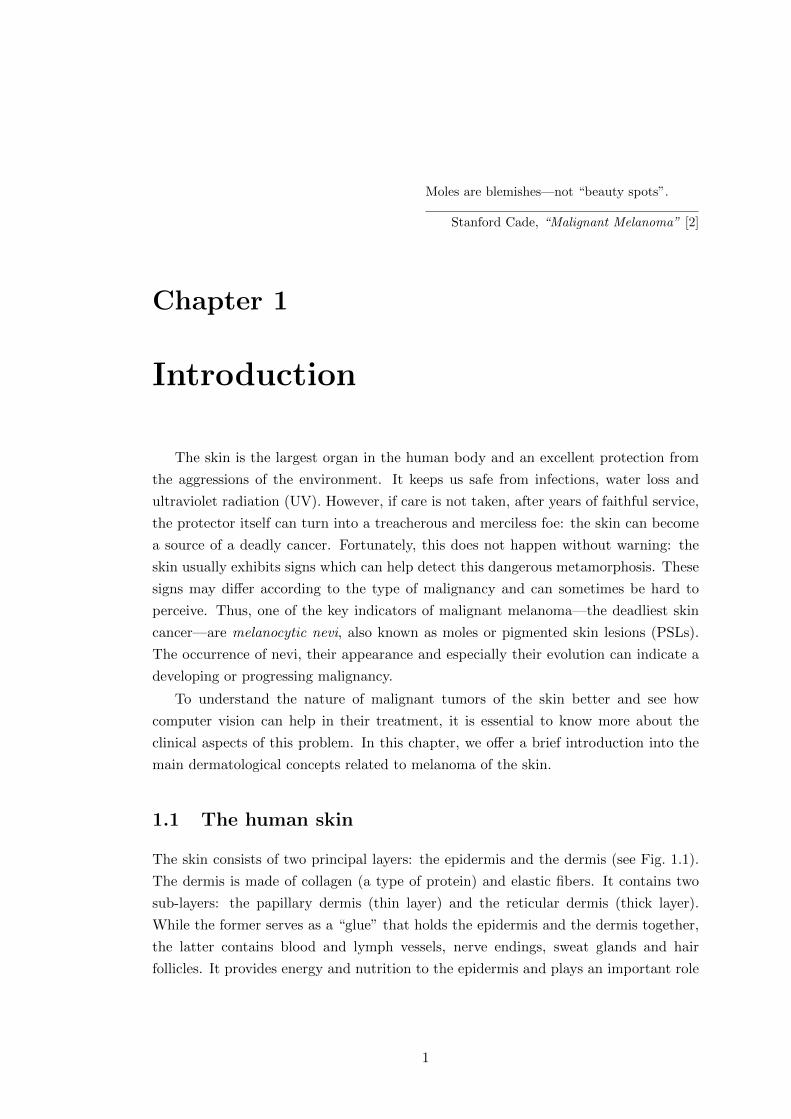
Figure 1.1: Anatomy of the skin showing the epidermis, the dermis, and subcutaneous (hypodermic)tissue. Illustration used with permission, copyright 2008 by Terese Winslow.
in thermoregulation, healing and the sense of touch [1].
The other layer, the epidermis, is a stratified squamous epithelium, a layered scale-
like tissue, which fulfills the protective functions of the skin. On simple morphological
grounds, the epidermis can be divided into four distinct layers from the bottom to the
top: stratum basale, stratum spinosum, stratum granulosum and stratum corneum [3].
There are four types of cells in the epidermis: keratinocytes, melanocytes, Langer-
hans’ cells and Merkel cells. Keratinocytes represent the majority (95%) of cells in
the epidermis and are the driving force for continuous renewal of the skin [3]. Their
abilities to divide and differentiate allow them to travel for approximately 30 days from
the basal layer (stratum basale) to the horny layer (stratum corneum). During this
time, the keratinocytes produced by division in the basal layer (here called basal cells)
move through the next layers transforming their morphology and biochemistry (differ-
entiation). As a result of this movement and transformation, the flattened cells without
nuclei, filled with keratin, come to form the outermost layer of the epidermis and are
called corneocytes. Finally, at the end of the differentiation program, the corneocytes
2
lose their cohesion and separate from the surface in the so-called desquamation process.
This is how our skin is constantly being renewed.
Merkel cells are probably derived from keratinocytes, but they act as mechano-
sensory receptors in response to touch forming close connections with sensory nerve
endings [3]. In turn, Langerhans’ cells are dendritic cells1 that detect foreign bodies
(antigens) that have penetrated the epidermis and deliver them to the local lymph
nodes.
In this project, the type of skin cells that most interest us are melanocytes. These
are dendritic cells found in the basal layer of the epidermis [3]. Unlike Langerhans’ cells,
melanocytes produce packages of melanin pigment and use their dendrites to distribute
them to surrounding keratinocytes (see Fig. 1.1). Besides protecting the subcutaneous2
tissue from being damaged by UV radiation, melanin also contributes to the color of
the skin (as well as that of the hair and eyes). Whenever the levels of UV radiation
increase, melanocytes start producing more melanin, hence our tanning reaction to sun
exposure.
Nevertheless, it is not the aesthetic results of melanocyte activity that draw our at-
tention, but their malignant transformation potential. Although cancer can develop in
almost any cell in the body, certain cells are more cancer-prone than others and the skin
is no exception. Most skin cancers develop from non-pigmented basal and squamous
keratinocytes. Their transformation results in basal cell carcinoma and squamous cell
carcinoma, respectively [1, 4]. However, melanocytes that undergo a malignant trans-
formation produce a less common but far more deadly and aggressive cancer: malignant
melanoma. The epidemiology and treatment of this cancer, as well as some skin lesions
known as its precursors, are described in the following sections.
1.2 Pigmented skin lesions
When melanocytes grow in clusters alongside normal cells, pigmented skin lesions or
melanocytic nevi appear on the surface of the skin [1] and are considered to be a normal
part of the skin. The most common benign PSLs are:
� Freckle or ephelis – a pale-brown, macular lesion, usually less than 3 mm in
1Dendritic cells have branched projections, the dendrites, that give them the name and a tree-likeappearance. Normally, cells of this kind are involved in processing and carrying antigen material tocells in the immune system.
2Subcutaneous – being, living, occurring, or administered under the skin (from sub- + Latin cutisskin). Definition by Merriam-Webster dictionary.
3
1. INTRODUCTION
(a)
(b)
(c)
(d)
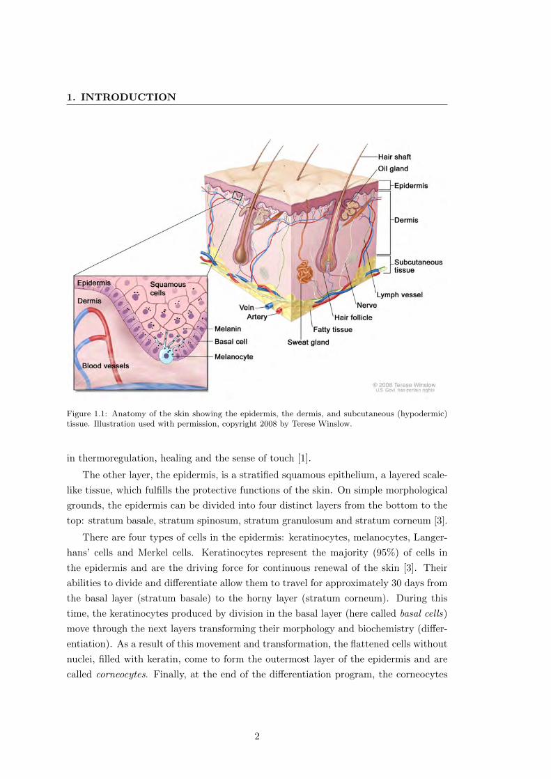
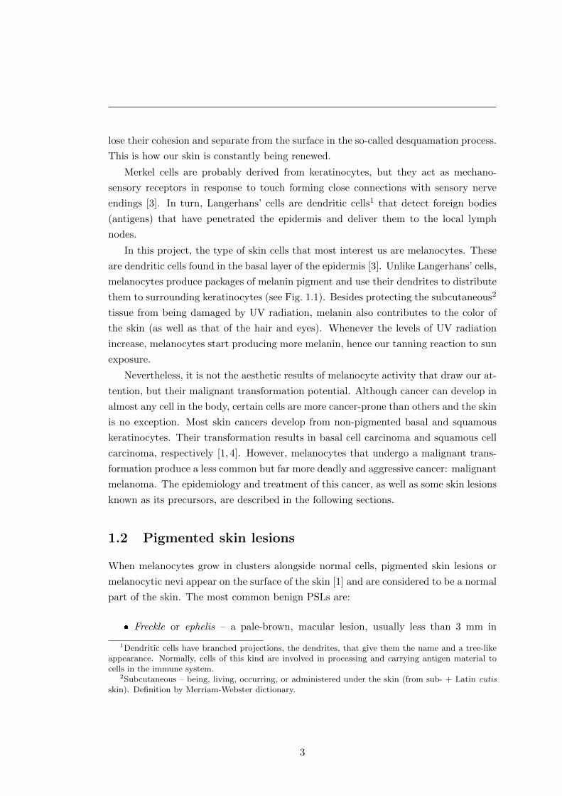
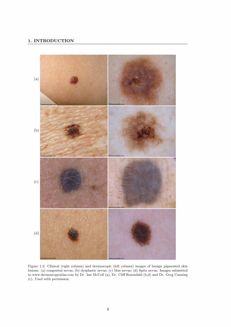
Figure 1.2: Clinical (right column) and dermoscopic (left column) images of benign pigmented skinlesions: (a) congenital nevus; (b) dysplastic nevus; (c) blue nevus; (d) Spitz nevus. Images submittedto www.dermoscopyatlas.com by Dr. Ian McColl (a), Dr. Cliff Rosendahl (b,d) and Dr. Greg Canning(c). Used with permission.
4

diameter with a poorly defined lateral margin, which appears and darkens on
light-exposed skin sites during periods of ultraviolet exposure [5].
� Common nevus – a typical flat melanocytic nevus or mole.
� Congenital nevus (Fig. 1.2a) – a mole that appears at birth, also known as “birth-
mark”.
� Atypical or dysplastic nevus (Fig. 1.2b) – a common nevus with inconsistent
coloration, irregular or notched edges, blurry borders, scale-like texture and a
diameter of over 5 mm [1]. Atypical mole syndrome, also known as “Familial
Atypical Multiple Mole Melanoma” (FAMMM) or dysplastic nevus syndrome,
describes individuals with large quantities of atypical nevi and possibly inherited
melanomas. The relative risk of developing a melanoma in such individuals is
around 6 to 10 times that of people with very few nevi [5].
� Blue nevus (Fig. 1.2c) – a melanocytic nevus comprised of aberrant collections
of benign pigment-producing melanocytes, located in the dermis rather than at
the dermoepidermal junction [5]. The optical effects of light reflecting off melanin
deep in the dermis provides its blue or blue-black appearance.
� Pigmented Spitz nevus (Fig. 1.2d) – an uncommon benign nevus, usually seen in
children, difficult to distinguish from melanoma [5].
Among these benign lesions, congenital and acquired dysplastic nevi are the known
precursors to malignant melanoma [6].
1.3 Malignant melanoma
In 1821, Dr. William Norris, a general practitioner in Stourbridge, England, described
the autopsy of a patient with what he thought was a fungoid disease: ”...thousands upon
thousands of coal black spots, of circular shapes and various sizes, were to be seen closely
dotting the shining mucous, serous, and fibrous membranes of most of the vital organs;
I should think the most dazzling sight ever beheld by morbid anatomist.” [7]. This
somewhat exalted description is one of the first documented clinical observations of a
metastasized malignant melanoma. Later, in 1857, Dr. Norris would state a number of
principles concerning the epidemiology, pathology and treatment of the disease, which
constitute the basic knowledge we have about melanoma to date [8].
5
1. INTRODUCTION
(a)
(b)
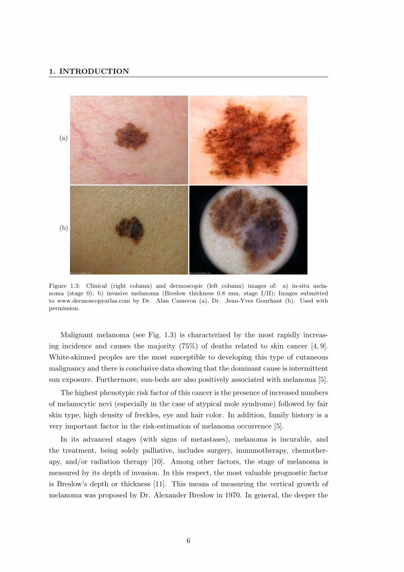
Figure 1.3: Clinical (right column) and dermoscopic (left column) images of: a) in-situ mela-noma (stage 0); b) invasive melanoma (Breslow thickness 0.8 mm, stage I/II); Images submittedto www.dermoscopyatlas.com by Dr. Alan Cameron (a), Dr. Jean-Yves Gourhant (b). Used withpermission.
Malignant melanoma (see Fig. 1.3) is characterized by the most rapidly increas-
ing incidence and causes the majority (75%) of deaths related to skin cancer [4, 9].
White-skinned peoples are the most susceptible to developing this type of cutaneous
malignancy and there is conclusive data showing that the dominant cause is intermittent
sun exposure. Furthermore, sun-beds are also positively associated with melanoma [5].
The highest phenotypic risk factor of this cancer is the presence of increased numbers
of melanocytic nevi (especially in the case of atypical mole syndrome) followed by fair
skin type, high density of freckles, eye and hair color. In addition, family history is a
very important factor in the risk-estimation of melanoma occurrence [5].
In its advanced stages (with signs of metastases), melanoma is incurable, and
the treatment, being solely palliative, includes surgery, immunotherapy, chemother-
apy, and/or radiation therapy [10]. Among other factors, the stage of melanoma is
measured by its depth of invasion. In this respect, the most valuable prognostic factor
is Breslow’s depth or thickness [11]. This means of measuring the vertical growth of
melanoma was proposed by Dr. Alexander Breslow in 1970. In general, the deeper the
6
measurement (depth of invasion), the higher the chances for metastasis and the worse
the prognosis.
Fortunately, early-stage melanoma (see Fig.1.3a) is highly curable [9]. In fact, the
results of Breslow’s experiments showed that lesions less than 0.76 mm thick do not
produce metastases [11]. This highlights the critical importance of timely diagnosis
and treatment of melanoma for patient survival [12].
Friedman et al. [6], the authors of the ABCD criteria for early melanoma detection,
emphasized in their paper that “by performing periodic complete cutaneous examina-
tions, by teaching patients the technique of routine self-examination of the skin, and
by proper use of diagnostic aids (particularly skin biopsy), physicians can improve the
chances for early diagnosis and prompt eradication of malignant melanoma”. Thus, the
importance of regular screening procedures for patients with a high risk of developing
melanoma is beyond doubt.
1.4 Melanoma screening
The prevailing strategy for skin screening procedures is total body skin examination
(TBSE) [13]. TBSE consists of meticulously analyzing every pigmented lesion on the
patient’s body and determining those which exhibit signs of a developing melanoma.
This can be a very tedious and time-consuming process (up to several hours), especially
for patients with atypical mole syndrome. To facilitate the recognition of melanoma
during the examination, dermatologists apply specific diagnostic rules and criteria as
well as using various imaging techniques. Furthermore, the application of artificial
intelligence to melanoma diagnosis allows the creation of systems for computer-aided
diagnosis.
1.4.1 Imaging techniques
Dermatologists use a number of non-invasive imaging techniques to help them diag-
nose skin lesions. Besides traditional photography, which has been used for a long
time in dermatology [14], there are a number of imaging modalities that allow the
visualization of different skin lesion structures. These modalities include dermoscopy,
confocal laser scanning microscopy, optical coherence tomography, high frequency ul-
trasound, positron emission tomography, magnetic resonance imaging and various spec-
troscopic imaging techniques, among others. For more information on all the imaging
modalities for melanoma diagnosis, the interested reader can refer to the available re-
views: [12,15–22].
7
1. INTRODUCTION
We have focused our research on the two imaging techniques most commonly used
in dermatological practice: clinical photography and dermoscopy.
1.4.1.1 Clinical photography
Dermatological photographs (digital or not) showing a single or multiple skin lesions on
the surface of the skin are referred to as clinical or macroscopic images. These images
reproduce what a clinician sees with the naked eye [23]. The left column in Figs. 1.2
and 1.3 demonstrate such macroscopic images. Clinical imaging is used to document
PSLs, mapping their location on the human body and tracking their changes over time
as sensitive signs of early melanoma [24].
Apart from taking photographs of single lesions or separate groups of lesions, physi-
cians may recur to total body photography, also known as total body skin imaging
(TBSI) and whole body photography (WBP) [13]. This is a method of photographic
documentation of a person’s entire cutaneous surface through a series of body sector
images.
During a TBSI procedure the patient should assume a set of standardized body
poses (see Fig. 1.4). The lighting conditions must be appropriate to allow the best
contrast between PSLs and the skin. In addition, the setup of a TBSI system should
be easily reproducible for successive acquisitions. The body parts that must be pho-
tographed are: the face, the neck, the area behind the ears, the scalp (in bald indi-
viduals), the anterior and posterior torso, and the extremities (including palms and
soles).
Advantages of total body skin imaging include [24]:
� potential aid for change identification in lesions not suspected at the time of
initial evaluation. The study conducted by Feit et al. [25] showed that TBSI
helped detect new and subtly changing melanomas which did not satisfy classical
clinical features of melanoma;
� efficient evaluation of large numbers of lesions;
� lack of reliance on expert interpretation of dermoscopic images.
Ideally, whole body photography should be systematically combined with other
techniques, including dermoscopy, for improved diagnostic efficiency and accuracy [24].
The study conducted in [26] showed that monitoring by total body photography and
sequential dermoscopy detects thinner melanomas.
8
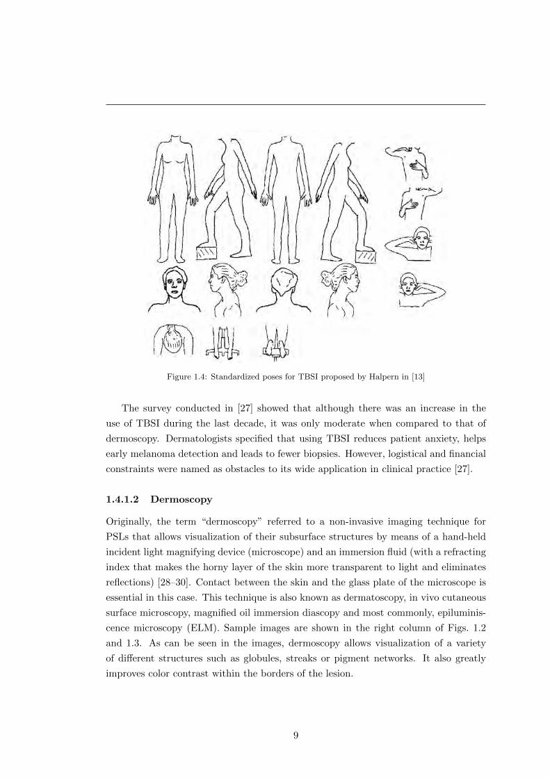
Figure 1.4: Standardized poses for TBSI proposed by Halpern in [13]
The survey conducted in [27] showed that although there was an increase in the
use of TBSI during the last decade, it was only moderate when compared to that of
dermoscopy. Dermatologists specified that using TBSI reduces patient anxiety, helps
early melanoma detection and leads to fewer biopsies. However, logistical and financial
constraints were named as obstacles to its wide application in clinical practice [27].
1.4.1.2 Dermoscopy
Originally, the term “dermoscopy” referred to a non-invasive imaging technique for
PSLs that allows visualization of their subsurface structures by means of a hand-held
incident light magnifying device (microscope) and an immersion fluid (with a refracting
index that makes the horny layer of the skin more transparent to light and eliminates
reflections) [28–30]. Contact between the skin and the glass plate of the microscope is
essential in this case. This technique is also known as dermatoscopy, in vivo cutaneous
surface microscopy, magnified oil immersion diascopy and most commonly, epiluminis-
cence microscopy (ELM). Sample images are shown in the right column of Figs. 1.2
and 1.3. As can be seen in the images, dermoscopy allows visualization of a variety
of different structures such as globules, streaks or pigment networks. It also greatly
improves color contrast within the borders of the lesion.
9
1. INTRODUCTION
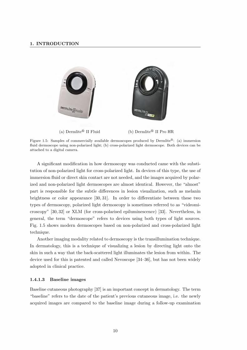
(a) Dermliter II Fluid (b) Dermliter II Pro HR
Figure 1.5: Samples of commercially available dermoscopes produced by Dermliter: (a) immersionfluid dermoscope using non-polarized light; (b) cross-polarized light dermoscope. Both devices can beattached to a digital camera.
A significant modification in how dermoscopy was conducted came with the substi-
tution of non-polarized light for cross-polarized light. In devices of this type, the use of
immersion fluid or direct skin contact are not needed, and the images acquired by polar-
ized and non-polarized light dermoscopes are almost identical. However, the “almost”
part is responsible for the subtle differences in lesion visualization, such as melanin
brightness or color appearance [30, 31]. In order to differentiate between these two
types of dermoscopy, polarized light dermoscopy is sometimes referred to as “videomi-
croscopy” [30, 32] or XLM (for cross-polarised epiluminescence) [33]. Nevertheless, in
general, the term “dermoscope” refers to devices using both types of light sources.
Fig. 1.5 shows modern dermoscopes based on non-polarized and cross-polarized light
technique.
Another imaging modality related to dermoscopy is the transillumination technique.
In dermatology, this is a technique of visualizing a lesion by directing light onto the
skin in such a way that the back-scattered light illuminates the lesion from within. The
device used for this is patented and called Nevoscope [34–36], but has not been widely
adopted in clinical practice.
1.4.1.3 Baseline images
Baseline cutaneous photography [37] is an important concept in dermatology. The term
“baseline” refers to the date of the patient’s previous cutaneous image, i.e. the newly
acquired images are compared to the baseline image during a follow-up examination
10
so that the evolution and/or appearance of new lesions can be detected. Baseline
images can be either clinical or dermoscopic, and do not in fact have to be limited to
photography: images acquired by any other means may have a baseline reference.
1.4.2 Melanoma diagnosis methods
During screening procedures, clinicians and dermatologists use certain criteria to de-
termine whether a given lesion is a melanoma. Performing the procedure without a
dermoscope or with the help of clinical baseline images, the ABCDE criteria [38] and
the Glasgow 7-point checklist [39] can be used.
The latter contains 7 criteria: 3 major (changes in size, shape and color) and 4
minor (diameter ≥ 7 mm, inflammation, crusting or bleeding and sensory change), but
has not been widely adopted [38]. The so-called ABCD criteria, proposed in 1985 by
Friedman et al. [6], have been extensively applied in clinical practice, mostly due to
simplicity of use [17, 38]. This mnemonic defines the diagnosis of a lesion based on its
asymmetry (A), irregularity of the border (B), color variegation (C) and the diameter
(D), that is generally greater than 6 mm for suspicious lesions. Later, in 2004, Abbasi et
al. [38] proposed expanding the ABCD criteria to ABCDE by incorporating the E for
“evolving” of the lesion over time, which reflects the results of the studies similar to the
one performed in [40, 41], and includes changes in features such as size, shape, surface
texture, color, etc.
In order to differentiate between melanoma and benign melanocytic tumors using
dermoscopic images, new diagnostic methods were created and existing clinical crite-
ria were adapted. These methods are summarized in Table 1.1. Note the identical
names of the criteria for different imaging modalities: ABCD rule of dermoscopy and
7-point checklist [42]. It is important to clearly differentiate between them to avoid
any confusion since they attempt to provide lesion diagnosis based on different types
of information.
To this end, Table 1.2 shows differences between methods of melanoma diagnosis
which share practically identical names but refer to different image modalities. As the
table illustrates, the modified meaning of the letters in the ABCD rule of dermoscopy
is: B for border sharpness and D for Differential structures. Importantly, besides these
changes, all the criteria in this method have a fairly different interpretation from their
clinical counterparts. Moreover, the “items” on the 7-point checklist differ completely
from those on the Glasgow 7-point checklist. Although the first three points on both
lists are awarded a higher score, they are all adapted specifically according to the
11
1. INTRODUCTION
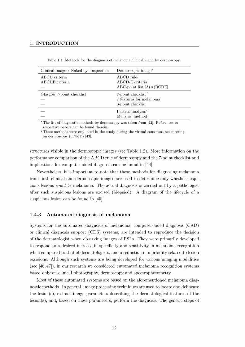
Table 1.1: Methods for the diagnosis of melanoma clinically and by dermoscopy.
Clinical image / Naked-eye inspection Dermoscopic image?
ABCD criteria ABCD rule�
ABCDE criteria ABCD-E criteria— ABC-point list [A(A)BCDE]
Glasgow 7-point checklist 7-point checklist�
— 7 features for melanoma— 3-point checklist
— Pattern analysis�
— Menzies’ method�
? The list of diagnostic methods by dermoscopy was taken from [42]. References torespective papers can be found therein.
� These methods were evaluated in the study during the virtual consensus net meetingon dermoscopy (CNMD) [43].
structures visible in the dermoscopic images (see Table 1.2). More information on the
performance comparison of the ABCD rule of dermoscopy and the 7-point checklist and
implications for computer-aided diagnosis can be found in [44].
Nevertheless, it is important to note that these methods for diagnosing melanoma
from both clinical and dermoscopic images are used to determine only whether suspi-
cious lesions could be melanoma. The actual diagnosis is carried out by a pathologist
after such suspicious lesions are excised (biopsied). A diagram of the lifecycle of a
suspicious lesion can be found in [45].
1.4.3 Automated diagnosis of melanoma
Systems for the automated diagnosis of melanoma, computer-aided diagnosis (CAD)
or clinical diagnosis support (CDS) systems, are intended to reproduce the decision
of the dermatologist when observing images of PSLs. They were primarily developed
to respond to a desired increase in specificity and sensitivity in melanoma recognition
when compared to that of dermatologists, and a reduction in morbidity related to lesion
excisions. Although such systems are being developed for various imaging modalities
(see [46, 47]), in our research we considered automated melanoma recognition systems
based only on clinical photography, dermoscopy and spectrophotometry.
Most of these automated systems are based on the aforementioned melanoma diag-
nostic methods. In general, image processing techniques are used to locate and delineate
the lesion(s), extract image parameters describing the dermatological features of the
lesion(s), and, based on these parameters, perform the diagnosis. The generic steps of
12
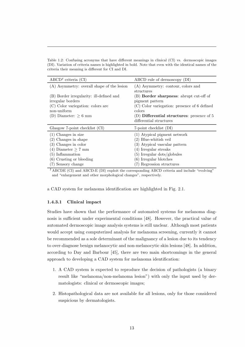
Table 1.2: Confusing acronyms that have different meanings in clinical (CI) vs. dermoscopic images(DI). Variation of criteria names is highlighted in bold. Note that even with the identical names of thecriteria their meaning is different for CI and DI.
ABCD� criteria (CI) ABCD rule of dermoscopy (DI)
(A) Asymmetry: overall shape of the lesion (A) Asymmetry: contour, colors andstructures
(B) Border irregularity: ill-defined andirregular borders
(B) Border sharpness: abrupt cut-off ofpigment pattern
(C) Color variegation: colors arenon-uniform
(C) Color variegation: presence of 6 definedcolors
(D) Diameter: ≥ 6 mm (D) Differential structures: presence of 5differential structures
Glasgow 7-point checklist (CI) 7-point checklist (DI)
(1) Changes in size (1) Atypical pigment network(2) Changes in shape (2) Blue-whitish veil(3) Changes in color (3) Atypical vascular pattern(4) Diameter ≥ 7 mm (4) Irregular streaks(5) Inflammation (5) Irregular dots/globules(6) Crusting or bleeding (6) Irregular blotches(7) Sensory change (7) Regression structures� ABCDE (CI) and ABCD-E (DI) exploit the corresponding ABCD criteria and include “evolving”
and “enlargement and other morphological changes”, respectively.
a CAD system for melanoma identification are highlighted in Fig. 2.1.
1.4.3.1 Clinical impact
Studies have shown that the performance of automated systems for melanoma diag-
nosis is sufficient under experimental conditions [48]. However, the practical value of
automated dermoscopic image analysis systems is still unclear. Although most patients
would accept using computerized analysis for melanoma screening, currently it cannot
be recommended as a sole determinant of the malignancy of a lesion due to its tendency
to over-diagnose benign melanocytic and non-melanocytic skin lesions [48]. In addition,
according to Day and Barbour [45], there are two main shortcomings in the general
approach to developing a CAD system for melanoma identification:
1. A CAD system is expected to reproduce the decision of pathologists (a binary
result like “melanoma/non-melanoma lesion”) with only the input used by der-
matologists: clinical or dermoscopic images;
2. Histopathological data are not available for all lesions, only for those considered
suspicious by dermatologists.
13
1. INTRODUCTION
The former is a methodological problem. It reflects the fact that a CAD system
is intended to diagnose a lesion without sufficient information for diagnosis or any
interaction with the dermatologist. This was highlighted by Dreiseitl et al. in their
study into the acceptance of CDS systems by dermatologists [49], i.e. that the currently
available CDS systems are designed to work “in parallel with and not in support of”
physicians, and because of this, only a few systems are found in routine clinical use.
Thus, an ideal CAD or CDS system for melanoma identification should reproduce the
decision of dermatologists (i.e. define the level of “suspiciousness” of a lesion) [45] and
provide dermatologists with comprehensive information regarding the grounds for this
decision [49].
1.5 Research motivation
Over the last 30 years, more people have had skin cancer than all other cancers com-
bined [50]. Accounting for less than 5% of these cases, melanoma causes the majority
of related deaths [10]. It is essential to take measures preventing the development of
this malignancy, but early detection of melanoma is vital.
Total body skin examination plays a primordial role in monitoring and detecting a
developing melanoma. However, non-automated screening of patients with large num-
bers of lesions (e.g., more than 50) can be very tedious and time-consuming. Expert
physicians have to examine every suspicious lesion for the typical signs of melanoma,
and use baseline images to detect those that had evolved. Thus, besides the difficulty of
identifying suspicious lesions, this procedure can also suffer from issues related to estab-
lishing correct body-to-image or image-to-image lesion correspondences. For example,
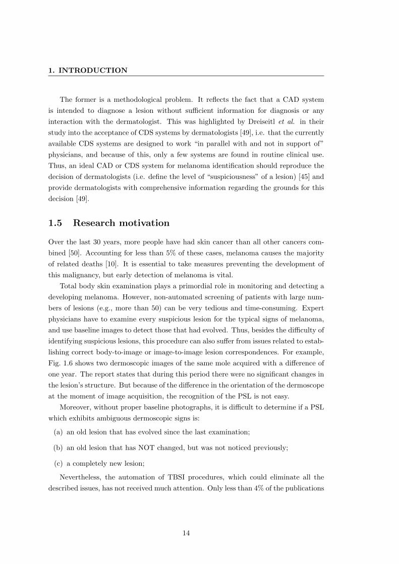
Fig. 1.6 shows two dermoscopic images of the same mole acquired with a difference of
one year. The report states that during this period there were no significant changes in
the lesion’s structure. But because of the difference in the orientation of the dermoscope
at the moment of image acquisition, the recognition of the PSL is not easy.
Moreover, without proper baseline photographs, it is difficult to determine if a PSL
which exhibits ambiguous dermoscopic signs is:
(a) an old lesion that has evolved since the last examination;
(b) an old lesion that has NOT changed, but was not noticed previously;
(c) a completely new lesion;
Nevertheless, the automation of TBSI procedures, which could eliminate all the
described issues, has not received much attention. Only less than 4% of the publications
14
Figure 1.6: Two dermoscopy images of a PSL acquired with a difference of one year using the sameimaging device (MoleMax�). No morphological change was reported. Images courtesy of Dr. J.Malvehy.
reviewed in this work (see Chapter 2) addressed the computerized analysis of multiple
skin lesions. It is possible that such a low percentage may be the consequence of
the specific nature of the problem. TBSI requires finding a trade-off between image
resolution and body coverage per image, where the resolution is governed by the needs
of change detection.
In spite of the fact that this trade-off is relatively easy to achieve with modern
cameras, and despite the development of total body photographic systems (e.g. [51,52]),
their automation stays mostly at the level of accessing and storing images. This lack
of attention and absence of research on completely automated systems for TBSI at
present seem unjustified considering the importance of this process in detecting early-
stage melanoma.
Therefore, this work attempts to fill the gap in research on computerized analysis
of multiple pigmented skin lesions, and open new perspectives for its application in
dermatological clinical practice. With the objective of facilitating the TBSE proce-
dures for patients and physicians, we designed and built a total body scanner allowing
for acquisition of skin surface images using cross-polarized light. It is capable of cap-
turing a set of 504 photographic images under controlled lighting conditions covering
approximately 85-90% of the body’s surface. For this scanner, we developed a frame-
work of algorithms for automated detection of pigmented skin lesions, their mapping in
three-dimensional space and consequent change detection between screening sessions.
Applied to the acquired images, these algorithms produce a precise map which links
images of individual PSLs with their real locations on the patient’s body, thus, solving
the body-to-image and image-to-image correspondence problems during TBSE.
15

1. INTRODUCTION
1.6 Thesis outline
This thesis describes the research work that resulted in the development and validation
of the algorithms for change detection in multiple nevi using the total body skin scanner.
Prior to designing the algorithms, we exhaustively studied the literature that exists in
the field of computerized analysis of pigmented skin lesions. Chapter 2 reports the
findings of this literature review.
Chapter 3 contains a description of the hardware design of the total body skin
scanner including the screening (image acquisition) and the extrinsic calibration (pat-
tern design and related image processing methodology) procedures.
Chapter 4 presents the software developed for PSL mapping and change detection.
The description is divided into two sections distinguishing the pipelines for intra- and
inter-exploration (examination) image processing.
Chapter 5 reports the results of testing all the algorithms on real datasets acquired
in laboratory and clinical settings, while Chapter 6 concludes this thesis.
Additional information on the techniques used in the implementation of the PSL
mapping and change detection pipelines can be found in the Appendix.
16
The measures science gives us in abundance are
to be used not timidly but bravely to combat
this pigmented foe, who claims the fairest and
the youngest and the old with equal impartial-
ity.
Stanford Cade, “Malignant Melanoma” [2]
Chapter 2
Computerized analysis of PSLs: a
literature review
In 1992, Stoecker and Moss summarized in their editorial the potential benefits of
applying digital imaging to dermatology [53]. These benefits were viewed according to
the technology available at the time, including of course the capabilities of computer
vision techniques, and the results of the earlier research in the area (e.g. [34, 54]).
Among others, these included objective non-invasive documentation of skin lesions,
systems for their diagnostic assistance by malignancy scoring, identifying changes, and
telediagnosis. This was the first time a journal had dedicated an entire special issue
to methods for computerized analysis of images in dermatology specifically applied
to skin cancer. Almost two decades later, the 2011 publication of the second special
issue,Advances in skin cancer image analysis [55], allowed us to clearly see the changes
that have taken place in this field. More importantly, we are able to see how close we
are to making certain benefits real rather than potential, and which ones have turned
out to be even more beneficial than initially predicted.
Such an overview can also reveal various problems in the way of achieving one of the
main goals—the creation of reliable automated means of assistance in melanoma diag-
nosis. Apart from the known methodological [45] and the dataset [56] problems, there
exists what we call a bibliography problem. While the research history of computerized
analysis of PSLs is vast and spread across hundreds of publications, comprehensive lit-
erature reviews are scarce. Yet without adequate material facilitating the assessment
of previous work, especially for those new to the field, researchers have to repeatedly
carry out the same work of article look-up, leaving less time for their analysis.
For this reason, we have attempted to create an extensive literature review estab-
17
2. COMPUTERIZED ANALYSIS OF PSLS: A LITERATURE REVIEW
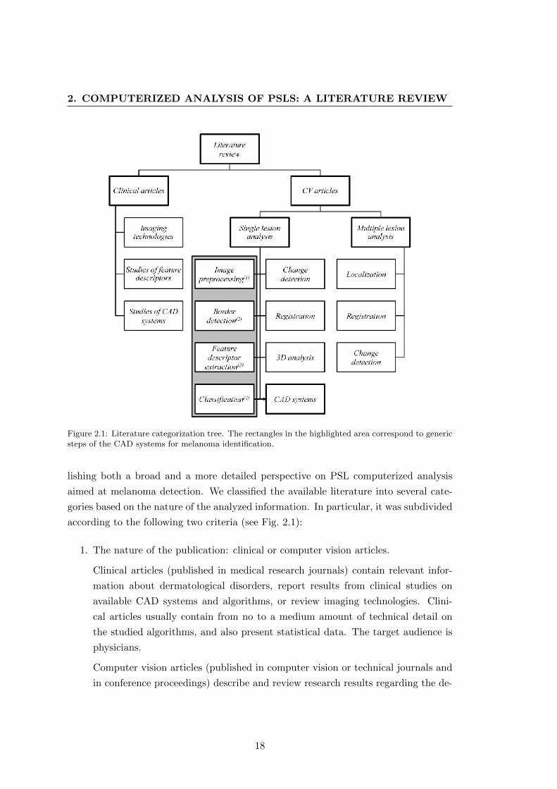
Figure 2.1: Literature categorization tree. The rectangles in the highlighted area correspond to genericsteps of the CAD systems for melanoma identification.
lishing both a broad and a more detailed perspective on PSL computerized analysis
aimed at melanoma detection. We classified the available literature into several cate-
gories based on the nature of the analyzed information. In particular, it was subdivided
according to the following two criteria (see Fig. 2.1):
1. The nature of the publication: clinical or computer vision articles.
Clinical articles (published in medical research journals) contain relevant infor-
mation about dermatological disorders, report results from clinical studies on
available CAD systems and algorithms, or review imaging technologies. Clini-
cal articles usually contain from no to a medium amount of technical detail on
the studied algorithms, and also present statistical data. The target audience is
physicians.
Computer vision articles (published in computer vision or technical journals and
in conference proceedings) describe and review research results regarding the de-
18
velopment of dermatological CAD systems. They contain a fair amount of techni-
cal detail on the algorithms. The target audience is computer vision researchers.
2. Number of analyzed lesions: single or multiple lesion analysis. This criterion
created a highly uneven distribution of computer vision papers, since less than
4% of all the reviewed papers are dedicated to multiple lesion analysis. This is
an important finding which clearly shows the main focus area in the field: the
analysis of dermoscopic/clinical images of single PSLs.
The detailed subdivision of the literature was based on the typical workflow steps of
CAD systems for melanoma recognition from single lesion images. Fig. 2.1 shows these
steps in the highlighted area, numbered according to their position in the workflow.
Other boxes in the figure represent literature/steps which usually do not form part of
CAD systems, although this is not always the case. Some systems [57, 58] actually
conduct lesion registration and change detection as a part of their workflow or as an
additional function. The category “CAD systems” contains articles describing archi-
tecture of automated melanoma diagnosis systems including all steps of the workflow,
whereas articles from other categories concentrate only on specific steps, but in more
detail. Note that the workflow is defined only for the systems used in single lesion
analysis.
The literature referenced in this work (with publication dates from 1984 to 2013) is
directly related to the computerized analysis of PSLs, and its distribution shows where
efforts have been concentrated in recent decades. Counting more than 400 publications
in total (this only includes papers found relevant for our review, not all of which are
referenced herein), the distribution of clinical to computer vision articles is approxi-
mately 24% to 76%, respectively. The reviewed clinical articles concern only single
PSL analysis, with the majority dedicated to CAD system studies (over 60%). In turn,
publications on “Multiple lesion analysis” are found only among the computer vision
articles. In the latter category, most papers on “Single lesion analysis” concentrate on
“Border detection” (28%) and “Feature extraction” (29%), 19% on “CAD systems”
and 16% on “Classification” categories. The rest of the papers were attributed to other
categories.
2.1 Single lesion analysis
This section reviews computerized analysis methods applied to images depicting a single
PSL. Each subsection below represents a category of the literature classification and
19
2. COMPUTERIZED ANALYSIS OF PSLS: A LITERATURE REVIEW
Table 2.1: PSL image preprocessing operations
Operation References
Artifact rejection
Hair [59–77]Air bubbles [60,68,78]Specular reflections [68,79]Ruler markings [64,68,78]Interlaced video misalignment [79]Various artifacts:
Median filter [57,80–85]Wiener filter [86]
Image enhancement
Color correction/calibration [87–91]Illumination correction [69,78,92–95]Contrast enhancement [96–99]Edge enhancement by KLT [80,82]
provides references to relevant publications and reviews.
2.1.1 Image preprocessing
After a clinical or dermoscopic image is acquired, it may not have the optimal quality for
subsequent analysis. The preprocessing step serves to compensate for the imperfections
of image acquisition and eliminate artifacts, such as hairs or ruler markings. Good
performance of the methods at this stage not only ensures correct behavior of the
algorithms in the following stages of analysis, but also relaxes the constraints on the
image acquisition process.
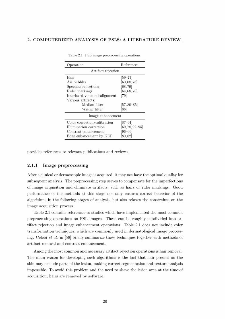
Table 2.1 contains references to studies which have implemented the most common
preprocessing operations on PSL images. These can be roughly subdivided into ar-
tifact rejection and image enhancement operations. Table 2.1 does not include color
transformation techniques, which are commonly used in dermatological image process-
ing. Celebi et al. in [56] briefly summarize these techniques together with methods of
artifact removal and contrast enhancement.
Among the most common and necessary artifact rejection operations is hair removal.
The main reason for developing such algorithms is the fact that hair present on the
skin may occlude parts of the lesion, making correct segmentation and texture analysis
impossible. To avoid this problem and the need to shave the lesion area at the time of
acquisition, hairs are removed by software.
20
A typical hair-removal algorithm comprises two steps: hair detection and hair repair
(restoration or “inpainting”). The latter consists in filling the image space occupied
by hair with proper intensity/color values. Its output greatly affects the quality of
the lesion’s border and texture. And since this information is indispensable for correct
diagnosis from dermoscopic images, it is important to ensure the best hair repair output.
The first widely adopted method of hair removal in dermoscopic images, DullRazor®,
was proposed in 1997 [59]. In 2011, Kiani and Sharafat [71] improved it to remove
light-colored hairs. While some of the approaches use generalized methods of super-
vised learning to detect and remove hairs [61, 72], others use more specific algorithms.
Recently, Abbas et al. [73] reviewed the existing methods and proposed a broad classifi-
cation into three groups based on their hair repair algorithm type: linear interpolation
techniques [59, 60, 63, 70], inpainting by nonlinear partial differential equations (PDE)
based diffusion algorithms [62,66,67,78] and exemplar-based methods [64,65,68]. Their
own hair repair method [73] used fast marching image inpainting, and was later im-
proved in [100].
Median filtering is widely used to suppress spurious noise, such as small pores on
the skin, shines and reflections [57, 81, 85], thin hairs or small air bubbles (minimizing
or completely removing them [80, 84]). Other artifacts in dermatological images also
include ruler markings, specular reflections and even video field misalignment caused
by interlaced cameras (see Table 2.1).
Of image enhancement operations, perhaps the most important one, from the point
of view of lesion diagnosis, is color correction or calibration. This operation consists
in recovering real colors of a photographed lesion, thus allowing for a more reliable use
of color information in manual and automatic diagnosis. Recent studies place special
emphasis on color correction in images with a joint photographic experts group (JPEG)
format (as opposed to raw image files) obtained using low-cost digital cameras [90,91].
Other operations in this category are illumination correction, and contrast and edge
enhancement. In order to perform the latter operation, Karhunen-Loeve transform
(KLT), also known as Hotelling Transform or principal component analysis (PCA), is
widely used.
2.1.2 Lesion border detection
An accurately detected border of a skin lesion is crucial for its automated diagnosis.
Therefore, border detection (segmentation) is one of the most active areas in the com-
puterized analysis of PSLs. A lot of effort has been made to improve lesion segmentation
21
2. COMPUTERIZED ANALYSIS OF PSLS: A LITERATURE REVIEW
algorithms and come up with adequate measures of their performance.
The problem of lesion border detection is not as trivial as it may seem. Firstly, since
dermatologists do not usually delineate lesion borders for diagnosis [45] there exists a
ground truth problem. Segmentation algorithms are intended to reproduce the way
human observers, who are generally not very good at discriminating between subtle
variations in contrast or blur [101], perceive the boundaries of a lesion. But because
of high inter- and intra-observer variability in PSL boundary perception among der-
matologists [101–103] the ground truth often lacks definiteness and has to be obtained
as a fusion of several manual segmentations. Secondly, the morphological structure
of a lesion itself (depigmentation, low lesion-to-skin gradient, multiple lesion regions,
etc.) can act as a confusion factor for both manual and automatic segmentation. These
problems have led to the development of a wide variety of PSL segmentation methods
which span all categories of segmentation algorithms [56].
These algorithms can be classified in many ways regarding, for instance, their level
of automation (automatic vs. semi-automatic), their number of parameters or the
required methods of postprocessing [56]. However, the purpose of this subsection is not
to review all these methods, but to provide information regarding available reviews and
comparisons and to emphasize the role of certain approaches to the problem.
2.1.2.1 PSL border detection methodology
Morphological differences in the appearance of PSLs in clinical and dermoscopic im-
ages directly influence the choice of method for border detection. Moreover, various
conditions, such as type of lesion, location, color conditions or angle of view, add to the
diverse difficulties in segmenting using the same imaging modality [56,60,104]. There-
fore, the available methods aim to provide robustness in difficult segmentation cases
adapting to specific conditions of the image type (e.g. [105]).
Clinical images One of the earliest works on skin lesion border detection was pub-
lished in 1989 and used the concept of spherical coordinates for color space represen-
tation [106]. Since then, it has been widely adopted in the literature for lesion feature
extraction and color segmentation. Comparisons of different color spaces applied to
segmentation were carried out in [107,108] and in [96].
In 1990, Golston et al. estimated the role of several determinants of the lesion bor-
der, namely color, luminance, texture and 3D information [109]. While 3D information
was mostly absent, color and luminance appeared to be the major factors for most of the
images. Thus, the authors discussed an overall algorithm that would take into account
22

several border determinants based on their level of confidence, and proposed a radial
search method based on luminance information. Similarly, in support of multifactorial
descriptiveness of the lesion border, Dhawan and Sicsu proposed combining grey-level
intensity and textural information [110]. Further works concentrated on improving ex-
isting techniques [111] and applying a multitude of different approaches, including edge
detection [104, 112], active contours [62], PDE [62, 67], gradient vector flow [113] and
many others.
Dermoscopic images Following the trend initiated by clinical images, multiple seg-
mentation algorithms and their combinations were investigated for dermoscopic im-
ages. Fleming et al. [60] discussed several implementations of segmentation algorithms.
Though agreeing that one of the most efficient border determinants is color, they pro-
posed an approach incorporating spatial and chromatic information to produce better
segmentations. After implementing and testing various algorithms, the final method
combined principal component transform, stabilized inverse diffusion equations and
thresholding in the green channel.
Later thresholding approaches became more sophisticated in comparison with the
relatively simple methods of single color channel thresholding proposed earlier [60,114].
Iterative thresholding [115], type-2 fuzzy logic based thresholding [116], fusion of thresh-
olds [117–119], hybrid [120], local entropy [121] and color histogram thresholding [122]
have been proposed recently. Many other approaches have been applied to the seg-
mentation of dermoscopic images. Among them are various algorithms using and
combining different categories of techniques, such as clustering [123–126], soft com-
puting (neural networks [115, 127,128] and evolution strategy [129]), supervised learn-
ing [61,72,130,131], active contours [33,132], and dynamic programming [74], to name
but a few.
Without doubt, all these (and other approaches not mentioned here) have their
advantages and drawbacks. However, it should be noted that most of the algorithms
are tested on various fairly small datasets, not many of which include special “difficult”
cases. Consequently, the performance assessment for these algorithms is not trivial,
especially based only on the results reported by the authors. In this respect, the
comparison studies allow these algorithms to be assessed in a more uniform framework,
clearly defining their strengths and weaknesses.
23
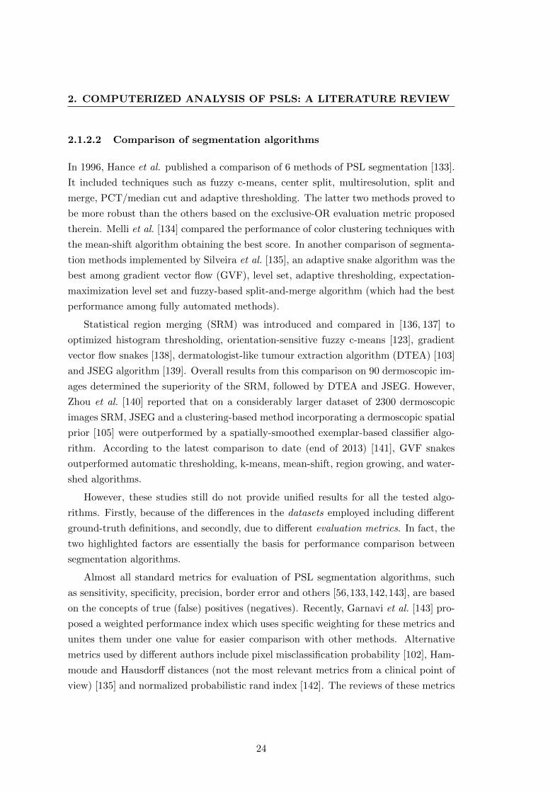
2. COMPUTERIZED ANALYSIS OF PSLS: A LITERATURE REVIEW
2.1.2.2 Comparison of segmentation algorithms
In 1996, Hance et al. published a comparison of 6 methods of PSL segmentation [133].
It included techniques such as fuzzy c-means, center split, multiresolution, split and
merge, PCT/median cut and adaptive thresholding. The latter two methods proved to
be more robust than the others based on the exclusive-OR evaluation metric proposed
therein. Melli et al. [134] compared the performance of color clustering techniques with
the mean-shift algorithm obtaining the best score. In another comparison of segmenta-
tion methods implemented by Silveira et al. [135], an adaptive snake algorithm was the
best among gradient vector flow (GVF), level set, adaptive thresholding, expectation-
maximization level set and fuzzy-based split-and-merge algorithm (which had the best
performance among fully automated methods).
Statistical region merging (SRM) was introduced and compared in [136, 137] to
optimized histogram thresholding, orientation-sensitive fuzzy c-means [123], gradient
vector flow snakes [138], dermatologist-like tumour extraction algorithm (DTEA) [103]
and JSEG algorithm [139]. Overall results from this comparison on 90 dermoscopic im-
ages determined the superiority of the SRM, followed by DTEA and JSEG. However,
Zhou et al. [140] reported that on a considerably larger dataset of 2300 dermoscopic
images SRM, JSEG and a clustering-based method incorporating a dermoscopic spatial
prior [105] were outperformed by a spatially-smoothed exemplar-based classifier algo-
rithm. According to the latest comparison to date (end of 2013) [141], GVF snakes
outperformed automatic thresholding, k-means, mean-shift, region growing, and water-
shed algorithms.
However, these studies still do not provide unified results for all the tested algo-
rithms. Firstly, because of the differences in the datasets employed including different
ground-truth definitions, and secondly, due to different evaluation metrics. In fact, the
two highlighted factors are essentially the basis for performance comparison between
segmentation algorithms.
Almost all standard metrics for evaluation of PSL segmentation algorithms, such
as sensitivity, specificity, precision, border error and others [56,133,142,143], are based
on the concepts of true (false) positives (negatives). Recently, Garnavi et al. [143] pro-
posed a weighted performance index which uses specific weighting for these metrics and
unites them under one value for easier comparison with other methods. Alternative
metrics used by different authors include pixel misclassification probability [102], Ham-
moude and Hausdorff distances (not the most relevant metrics from a clinical point of
view) [135] and normalized probabilistic rand index [142]. The reviews of these metrics
24
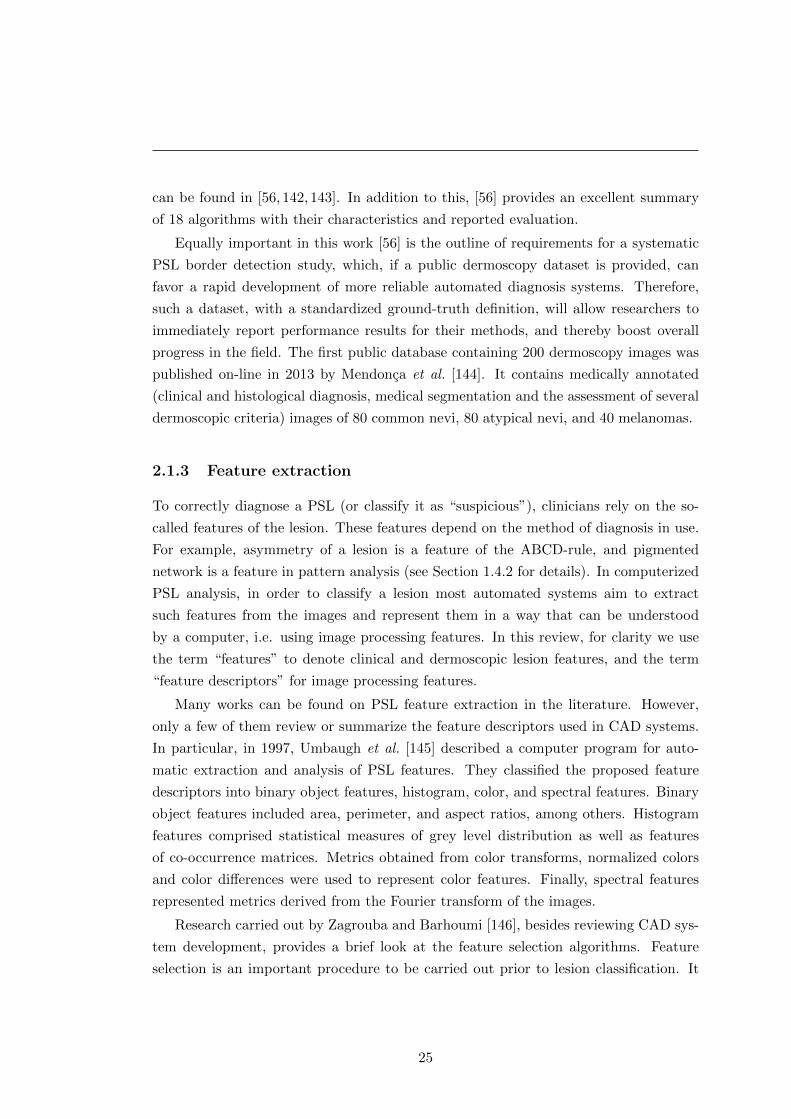
can be found in [56, 142, 143]. In addition to this, [56] provides an excellent summary
of 18 algorithms with their characteristics and reported evaluation.
Equally important in this work [56] is the outline of requirements for a systematic
PSL border detection study, which, if a public dermoscopy dataset is provided, can
favor a rapid development of more reliable automated diagnosis systems. Therefore,
such a dataset, with a standardized ground-truth definition, will allow researchers to
immediately report performance results for their methods, and thereby boost overall
progress in the field. The first public database containing 200 dermoscopy images was
published on-line in 2013 by Mendonca et al. [144]. It contains medically annotated
(clinical and histological diagnosis, medical segmentation and the assessment of several
dermoscopic criteria) images of 80 common nevi, 80 atypical nevi, and 40 melanomas.
2.1.3 Feature extraction
To correctly diagnose a PSL (or classify it as “suspicious”), clinicians rely on the so-
called features of the lesion. These features depend on the method of diagnosis in use.
For example, asymmetry of a lesion is a feature of the ABCD-rule, and pigmented
network is a feature in pattern analysis (see Section 1.4.2 for details). In computerized
PSL analysis, in order to classify a lesion most automated systems aim to extract
such features from the images and represent them in a way that can be understood
by a computer, i.e. using image processing features. In this review, for clarity we use
the term “features” to denote clinical and dermoscopic lesion features, and the term
“feature descriptors” for image processing features.
Many works can be found on PSL feature extraction in the literature. However,
only a few of them review or summarize the feature descriptors used in CAD systems.
In particular, in 1997, Umbaugh et al. [145] described a computer program for auto-
matic extraction and analysis of PSL features. They classified the proposed feature
descriptors into binary object features, histogram, color, and spectral features. Binary
object features included area, perimeter, and aspect ratios, among others. Histogram
features comprised statistical measures of grey level distribution as well as features
of co-occurrence matrices. Metrics obtained from color transforms, normalized colors
and color differences were used to represent color features. Finally, spectral features
represented metrics derived from the Fourier transform of the images.
Research carried out by Zagrouba and Barhoumi [146], besides reviewing CAD sys-
tem development, provides a brief look at the feature selection algorithms. Feature
selection is an important procedure to be carried out prior to lesion classification. It
25
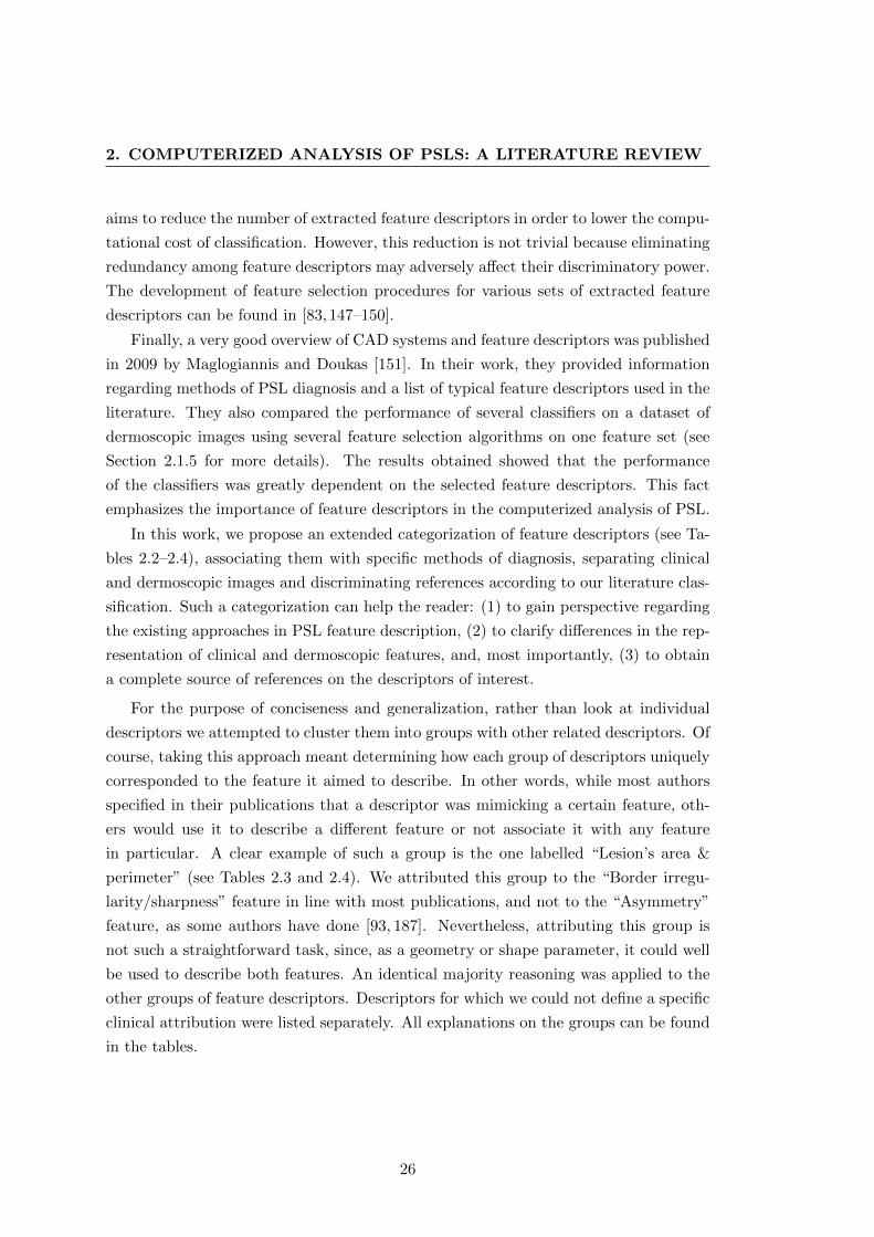
2. COMPUTERIZED ANALYSIS OF PSLS: A LITERATURE REVIEW
aims to reduce the number of extracted feature descriptors in order to lower the compu-
tational cost of classification. However, this reduction is not trivial because eliminating
redundancy among feature descriptors may adversely affect their discriminatory power.
The development of feature selection procedures for various sets of extracted feature
descriptors can be found in [83,147–150].
Finally, a very good overview of CAD systems and feature descriptors was published
in 2009 by Maglogiannis and Doukas [151]. In their work, they provided information
regarding methods of PSL diagnosis and a list of typical feature descriptors used in the
literature. They also compared the performance of several classifiers on a dataset of
dermoscopic images using several feature selection algorithms on one feature set (see
Section 2.1.5 for more details). The results obtained showed that the performance
of the classifiers was greatly dependent on the selected feature descriptors. This fact
emphasizes the importance of feature descriptors in the computerized analysis of PSL.
In this work, we propose an extended categorization of feature descriptors (see Ta-
bles 2.2–2.4), associating them with specific methods of diagnosis, separating clinical
and dermoscopic images and discriminating references according to our literature clas-
sification. Such a categorization can help the reader: (1) to gain perspective regarding
the existing approaches in PSL feature description, (2) to clarify differences in the rep-
resentation of clinical and dermoscopic features, and, most importantly, (3) to obtain
a complete source of references on the descriptors of interest.
For the purpose of conciseness and generalization, rather than look at individual
descriptors we attempted to cluster them into groups with other related descriptors. Of
course, taking this approach meant determining how each group of descriptors uniquely
corresponded to the feature it aimed to describe. In other words, while most authors
specified in their publications that a descriptor was mimicking a certain feature, oth-
ers would use it to describe a different feature or not associate it with any feature
in particular. A clear example of such a group is the one labelled “Lesion’s area &
perimeter” (see Tables 2.3 and 2.4). We attributed this group to the “Border irregu-
larity/sharpness” feature in line with most publications, and not to the “Asymmetry”
feature, as some authors have done [93, 187]. Nevertheless, attributing this group is
not such a straightforward task, since, as a geometry or shape parameter, it could well
be used to describe both features. An identical majority reasoning was applied to the
other groups of feature descriptors. Descriptors for which we could not define a specific
clinical attribution were listed separately. All explanations on the groups can be found
in the tables.
26
Table 2.2: Feature extraction for pattern analysis [42].
Pattern analysis References
Glo
bal
patt
erns Reticular [152–154] [155]a [156]b
Globular [152–154,157] [155] [156]Cobblestone [153,157] [155]Homogeneous [152–154,157] [155] [156]Starburst [155]Parallel [153,157][155]Multicomponent [154]Non-specific —
Loca
lfe
atu
res
Pigment network [60,72,158–165] [166–168]c [58]b
Dots/globules [60,61,169] [58]Streaks [170,171] [166,172]c
Blue-whitish veil [173–176] [172,177,178]c
Regression structures [61,179,180] [172,177,178] [181]b
Hypopigmentation [61] [181]
Blotches [182–184] [185]d
Vascular structures [186]a Computer vision article from the ”Classification” categoryb Computer vision article from the ”CAD systems” categoryc Feature extraction following the 7-Point checklist for
dermoscopyd Clinical article from the ”Studies of lesion features” category
Among the diagnosis methods considered were the ABCD-rule and pattern analysis
for dermoscopic images, and the ABCDE criteria for clinical images. Table 2.2 contains
references to articles aimed at computing descriptors for pattern analysis features [42].
The majority of the papers referenced in this table belong to the “Feature extraction”
category. Among these, a number were dedicated to feature extraction following the
7-point checklist method for melanoma diagnosis from dermoscopic images [166–168,
172,177,178]. A preliminary study on detection of some dermoscopic structures (blue-
whitish veil, atypical pigmented network and irregular pigmentation) can be found
in [44].
Descriptors of features used in the ABCD-rule of dermoscopy and the ABCDE clini-
cal criteria are summarized in Tables 2.3 and 2.4. This separate representation helps to
highlight differences and similarities in the computerized description of these features.
As illustrated by these two tables, the largest groups of feature descriptors are present
in both types of images (clinical and dermoscopy) and define the similarities. The differ-
ences, on the other hand, can be seen in smaller groups or even individual descriptors.
For example, dermoscopic interest points [250], size functions [247–249], scale-invariant
27

2. COMPUTERIZED ANALYSIS OF PSLS: A LITERATURE REVIEWT
able
2.3
:D
erm
osc
opic
featu
res
of
pig
men
ted
skin
lesi
ons
acc
ord
ing
toA
BC
Dru
leof
der
mosc
opy
[42,2
43]
and
thei
rdes
crip
tors
Der
mosc
op
icfe
atu
res
Fea
ture
des
crip
tors
Clin
ical
refe
ren
ces
Com
pu
ter
vis
ion
refe
ren
ces
Fea
ture
saC
AD
syst
emsa
Fea
ture
sbL
esio
ncl
ass
ifica
tion
CA
Dsy
stem
sb
Asy
mm
etry
Les
ion
’sce
ntr
oid
&m
om
ents
of
iner
tiac
[185,1
88–191]
[114,1
92–197]
[174,1
98]
[199–203]
[82,8
3,2
04–208]
Review:[209]
Sym
met
rym
ap
s—
—[2
10]
—[6
3]
Fou
rier
des
crip
tors
——
[211]
——
Glo
bal
poin
tsi
gn
atu
res
(GP
S)
——
[212]
——
Oth
ersy
mm
etry
des
crip
tors
[191,2
13]
[214,2
15]
[216]
[187]
[86,2
17,2
18]
Bord
ersh
arp
nes
sL
esio
n’s
are
a&
per
imet
erd
[185,1
88,1
89]
[192,1
95–197]
[174]
[187,1
99–203]
[82,8
3,8
6,2
04,
206–208,2
17]
Convex
hu
lld
escr
ipto
rse
——
——
[83,8
6]
Bou
nd
ing
box
des
crip
tors
e—
——
[202,2
03]
[83,2
04,2
06]
Fra
ctal
geo
met
ryf
—[1
96]
[219]
[199,2
00]
[82,8
6]
Gra
die
nt-
base
dd
escr
ipto
rs[1
90]
[114,2
14]
[216,2
20,
221]
[187,2
01]
[57,8
6,2
04–207,
217,2
18]
Mu
lti-
scale
rou
gh
nes
sd
escr
ipto
rs—
—[2
22]
——
Colo
rvari
egati
on
RG
Bst
ati
stic
al
des
crip
tors
g—
[193–197,2
14,
215]
[176,2
16,
223,2
24]
[187,1
99–203,2
25,2
26]
[83,8
6,2
07,2
08,
217]
Alt
ern
ati
ve
colo
rsp
ace
des
crip
tors
h[1
90]
[192,1
96,2
14]
[216,2
23,
224]
[187,2
00–203,2
25,2
26]
[83,2
04,2
06–208,
217,2
27,2
28]
Mu
nse
llco
lor
space
des
crip
tors
——
——
[229]
Gen
eralize
dco
lor
mom
ents
——
[224]
——
Rel
ati
ve
colo
rst
ati
stic
al
des
crip
tors
i—
[214]
[174,2
30]
[187]
[206,2
17,2
18]
Colo
rqu
anti
zati
onj
[188,1
89,2
09,
231]
[192,1
96,2
14]
[216,2
24,
230,2
32,2
33]
[187,2
00,2
02,2
34]
[82,2
05,2
06,2
17,
228,2
29]
Diff
eren
tial
stru
ctu
res
Mu
ltid
im.
rece
pti
ve
fiel
ds
his
togra
ms
——
—[2
34]
—
Oth
erW
avel
et-b
ase
dd
escr
ipto
rs—
—[2
35]
[202,2
26,2
36–241]
[58,8
1]
Gab
or
filt
erd
escr
ipto
rs—
[195]
—[1
99,2
25,2
42]
[228]
Inte
nsi
tyd
istr
ibu
tion
des
crip
tors
—[1
93,1
94,2
14]
[216]
[187]
[204,2
17,2
18]
Hara
lick
des
crip
tors
k—
[193,1
94,2
14]
[163,1
74,
216]
[187,2
01,2
03]
[83,2
07,2
17,2
18,
227–229]
28

Table
2.3
:D
erm
osc
opic
featu
res
of
pig
men
ted
skin
lesi
ons.
(continued)
Der
mosc
op
icfe
atu
res
Fea
ture
des
crip
tors
Clin
ical
refe
ren
ces
Com
pu
ter
vis
ion
refe
ren
ces
Fea
ture
saC
AD
syst
emsa
Fea
ture
sbL
esio
ncl
ass
ifica
tion
CA
Dsy
stem
sb
Loca
lb
inary
patt
ern
(LB
P)
——
[244]
[245]
—V
ari
ou
ste
xtu
red
escr
ipto
rs—
—[2
44]
[246]
[228]
Siz
efu
nct
ion
s—
[247]
—[2
48,2
49]
—S
IFT
an
dco
lor
SIF
T—
——
[226]
—D
erm
osc
op
icin
tere
stp
oin
ts—
—[2
50]
——
Bag-o
f-fe
atu
res
fram
ework
——
—[2
26,2
28,2
42]
—
aC
lin
ical
pap
ers
des
crib
ing
stu
die
sof
PS
Lfe
atu
red
escr
ipto
rsan
dC
AD
syst
ems,
resp
ecti
vel
yb
Com
pu
ter
vis
ion
pap
ers
des
crib
ing
PS
Lfe
atu
reex
tract
ion
an
dd
esig
nof
CA
Dsy
stem
s,re
spec
tivel
y
cT
his
gro
up
incl
ud
esall
mea
sure
sb
ase
don
com
pu
tin
gp
rin
cip
al
an
d/or
sym
met
ryaxes
,an
dce
ntr
oid
of
the
lesi
on
.A
sym
met
ryin
dex
/pe
rcen
tage
[151],
asp
ect
rati
o(l
engt
hen
ing)
,ra
dia
ld
ista
nce
dis
trib
uti
on
are
am
on
goth
erd
escr
ipto
rsin
the
gro
up
.d
Th
ese
des
crip
tors
defi
ne
the
rela
tion
bet
wee
nth
eare
aan
dp
erim
eter
of
an
ob
ject
,an
dth
us,
des
crib
eit
ssy
mm
etri
cal
an
db
ord
erch
ara
cter
isti
cs.
In
part
icu
lar,
itin
clu
des
ad
escr
ipto
rkn
ow
nas
com
pact
nes
sin
dex
/ra
tio
or
rou
nd
nes
s(I
=P
2/4πA
orI
=4πP
2/A
),as
wel
las
circ
ula
rity
,th
inn
ess
rati
oor
regu
lari
ty(I
=4πA/P
2).
Ines
sen
ce,
thes
era
tios
rep
rese
nt
on
ed
escr
ipto
r.e
Th
ere
are
vari
ou
sd
escr
ipto
rsb
ase
don
the
convex
hu
ll(C
H)
an
db
ou
nd
ing
box
(BB
)of
ale
sion
.In
part
icu
lar,
exte
nt
isth
era
tio
of
the
are
aof
the
lesi
on
toth
eare
aof
its
CH
(sam
eas
soli
dit
y)
or
BB
(sam
eas
rect
an
gula
rity
),w
her
eas
con
vexi
tyis
the
rati
oof
the
per
imet
erof
the
CH
toth
ep
erim
eter
of
the
lesi
on
,an
del
on
gati
on
isth
era
tio
bet
wee
nth
eh
eight
an
dth
ew
idth
of
the
BB
.f
Fra
cta
lge
om
etry
gro
up
incl
ud
esF
ou
rier
(fra
ctal)
dim
ensi
on
[251]
an
dla
cun
ari
ty[8
6].
gR
GB
des
crip
tors
enco
mp
ass
stati
stic
al
info
rmati
on
from
the
RG
Bch
an
nel
sin
the
form
of
such
valu
esas
min
/m
ax,
aver
age,
vari
an
ce,
entr
opy,
ener
gy,
ku
rtosi
s,ra
nge
an
doth
ers.
hA
lter
na
tive
colo
rsp
ace
des
crip
tors
incl
ud
ep
ara
met
ers
(sta
tist
ical
or
not)
der
ived
from
non
-RG
Bco
lor
space
s(e
xce
pt
for
norm
alise
dR
GB
)-
HS
V/H
SI
(hu
e,sa
tura
tion
,valu
e/in
ten
sity
),sp
her
ical
coord
inate
s[1
06],
CIE
LU
Van
doth
ers.
iT
his
gro
up
com
pri
ses
des
crip
tors
base
don
rela
tive
colo
r,su
chas
stati
stic
son
rela
tive
diff
eren
ce,
rati
oan
dch
rom
ati
city
[174]
of
sep
ara
teco
lor
chan
nel
s,
most
lyin
RG
Bco
lor
space
.j
Co
lor
qua
nti
zati
on
des
crip
tors
refe
rto
featu
res
ob
tain
edaft
erre
du
ctio
nof
the
qu
anti
tyof
colo
rsin
the
image.
Th
isre
du
ctio
nor
qu
anti
zati
on
can
be
don
e
usi
ng
colo
rp
roto
typ
es,
his
togra
ms
or
clu
ster
ing.
Typ
ical
des
crip
tors
incl
ud
en
um
ber
of
colo
rsan
dpe
rcen
tm
ela
no
ma
colo
r.k
Des
crip
tors
base
don
co-o
ccu
rren
cem
atr
ices
.T
hes
eco
nta
inen
tro
py,
iner
tia,
corr
ela
tio
n,
inve
rse
diff
eren
cean
doth
erst
ati
stic
al
para
met
ers.
29

2. COMPUTERIZED ANALYSIS OF PSLS: A LITERATURE REVIEW
Table
2.4
:C
linic
al
featu
res
of
pig
men
ted
skin
lesi
ons
acc
ord
ing
toA
BC
DE
crit
eria
[38,4
2]
and
thei
rdes
crip
tors
Clin
ical
featu
res
Fea
ture
des
crip
tors
Clin
ical
refe
ren
ces
Com
pu
ter
vis
ion
refe
ren
ces
CA
Dsy
stem
saF
eatu
reex
tract
ion
Les
ion
class
ifica
tion
CA
Dsy
stem
sb
Asy
mm
etry
Les
ion
’sce
ntr
oid
&m
om
ents
of
iner
tiac
[252]
[253–256]
[257–261]
[80,9
2,9
3,1
46,1
48,2
62–267]
Sym
met
ryd
ista
nce
(SD
)—
[268,2
69]
——
Bord
erir
regu
lari
tyL
esio
n’s
are
a&
per
imet
erd
[54,2
52,2
70–274]
[254–256,2
68,2
75–277]
[257–261]
[80,9
2,9
3,1
46,1
48,2
62–267,
278]
Convex
hu
lle
[272,2
73]
——
[92,9
3,1
48,2
66]
Bou
nd
ing
boxe
[270]
——
[92,9
3]
Fra
ctal
geo
met
ryf
[252]
[251,2
79–282]
—[8
0,1
46]
Gra
die
nt-
base
dd
escr
ipto
rs[5
4,2
71]
——
[80,9
2,9
3,1
46]
Irre
gu
lari
tyin
dex
—[2
83,2
84]
—S
igm
a-r
ati
o—
[285]
——
Bes
t-fi
tel
lip
se—
[256]
—[2
66]
Fou
rier
featu
re—
[255]
——
Poly
gon
al
ap
pro
xim
ati
on
—[2
76]
——
Con
dit
ion
al
entr
opy
—[2
86]
——
Hid
den
Mark
ov
mod
els
—[2
87]
——
Wavel
ettr
ansf
orm
—[2
88]
——
Cen
troid
dis
tan
ced
iagra
m—
[289]
——
Colo
rvari
egati
on
RG
Bst
ati
stic
al
des
crip
tors
g[5
4,2
52,2
71]
[149,2
55,2
56,2
77,2
90]
[257–260,2
91]
[92,2
62,2
64,2
65,2
67]
Alt
ern
ati
ve
colo
rsp
ace
des
crip
tors
h[2
70,2
92]
[255,2
90,2
93]
[257,2
58,2
60,
261]
[262,2
64,2
65,2
67,2
78]
Ow
nch
an
nel
rep
rese
nta
tion
——
—[9
3]
Rel
ati
ve
colo
rst
ati
stic
al
des
crip
tors
i—
[149,2
55,2
90,2
93,2
94]
[257,2
58]
[262,2
65,2
67]
Colo
rqu
anti
zati
onj
—[1
49,2
90,2
94–296]
[259]
[92,2
78]
Colo
rh
om
ogen
eity
,p
hoto
met
ry-g
eom
etry
corr
elati
on
——
—[8
0,1
46]
Para
met
ric
map
s—
[297]
——
Dia
met
erS
emi-
ma
jor
axis
of
the
bes
t-fi
tel
lip
se—
[256]
——
Evolv
ing
——
——
—
30

Table
2.4
:C
linic
al
featu
res
of
pig
men
ted
skin
lesi
ons(continued)
Oth
erfe
atu
res
Inte
nsi
tyd
istr
ibu
tion
des
crip
tors
[252,2
72–274,2
98]
——
[263,2
66]
Skin
patt
ern
an
aly
sis
—[2
56,2
99–303]
—H
ara
lick
des
crip
tors
k[2
70]
[304]
—[9
2,2
78]
Vari
ou
ste
xtu
red
escr
ipto
rs—
[305]
——
Wavel
et-b
ase
dd
escr
ipto
rs—
—[3
06]
—In
dep
end
ent
com
pon
ent
an
aly
sis
base
dd
escr
ipto
r—
—[2
91]
—
Ten
sor
dec
om
posi
tion
—[3
07]
——
aC
lin
ical
pap
ers
des
crib
ing
stu
die
sof
PS
Lfe
atu
red
escr
ipto
rsan
dC
AD
syst
ems,
resp
ecti
vel
yb
Com
pu
ter
vis
ion
pap
ers
des
crib
ing
PS
Lfe
atu
reex
tract
ion
an
dd
esig
nof
CA
Dsy
stem
s,re
spec
tivel
y
cT
his
gro
up
incl
ud
esall
mea
sure
sb
ase
don
com
pu
tin
gp
rin
cip
al
an
d/or
sym
met
ryaxes
,an
dce
ntr
oid
of
the
lesi
on
.A
sym
met
ryin
dex
/pe
rcen
tage
[151],
asp
ect
rati
o(l
engt
hen
ing)
,ra
dia
ld
ista
nce
dis
trib
uti
on
are
am
on
goth
erd
escr
ipto
rsin
the
gro
up
.d
Th
ese
des
crip
tors
defi
ne
the
rela
tion
bet
wee
nth
eare
aan
dp
erim
eter
of
an
ob
ject
,an
dth
us,
des
crib
eit
ssy
mm
etri
cal
an
db
ord
erch
ara
cter
isti
cs.
In
part
icu
lar,
itin
clu
des
ad
escr
ipto
rkn
ow
nas
com
pact
nes
sin
dex
/ra
tio
or
rou
nd
nes
s(I
=P
2/4πA
orI
=4πP
2/A
),as
wel
las
circ
ula
rity
,th
inn
ess
rati
oor
regu
lari
ty(I
=4πA/P
2).
Ines
sen
ce,
thes
era
tios
rep
rese
nt
on
ed
escr
ipto
r.e
Th
ere
are
vari
ou
sd
escr
ipto
rsb
ase
don
the
convex
hu
ll(C
H)
an
db
ou
nd
ing
box
(BB
)of
ale
sion
.In
part
icu
lar,
exte
nt
isth
era
tio
of
the
are
aof
the
lesi
on
toth
eare
aof
its
CH
(sam
eas
soli
dit
y)
or
BB
(sam
eas
rect
an
gula
rity
),w
her
eas
con
vexi
tyis
the
rati
oof
the
per
imet
erof
the
CH
toth
ep
erim
eter
of
the
lesi
on
,an
del
on
gati
on
isth
era
tio
bet
wee
nth
eh
eight
an
dth
ew
idth
of
the
BB
.f
Fra
cta
lge
om
etry
gro
up
incl
ud
esF
ou
rier
(fra
ctal)
dim
ensi
on
[251]
an
dla
cun
ari
ty[8
6].
gR
GB
des
crip
tors
enco
mp
ass
stati
stic
al
info
rmati
on
from
the
RG
Bch
an
nel
sin
the
form
of
such
valu
esas
min
/m
ax,
aver
age,
vari
an
ce,
entr
opy,
ener
gy,
ku
rtosi
s,ra
nge
an
doth
ers.
hA
lter
na
tive
colo
rsp
ace
des
crip
tors
incl
ud
ep
ara
met
ers
(sta
tist
ical
or
not)
der
ived
from
non
-RG
Bco
lor
space
s(e
xce
pt
for
norm
alise
dR
GB
)-
HS
V/H
SI
(hu
e,sa
tura
tion
,valu
e/in
ten
sity
),sp
her
ical
coord
inate
s[1
06],
CIE
LU
Van
doth
ers.
iT
his
gro
up
com
pri
ses
des
crip
tors
base
don
rela
tive
colo
r,su
chas
stati
stic
son
rela
tive
diff
eren
ce,
rati
oan
dch
rom
ati
city
[174]
of
sep
ara
teco
lor
chan
nel
s,
most
lyin
RG
Bco
lor
space
.j
Co
lor
qua
nti
zati
on
des
crip
tors
refe
rto
featu
res
ob
tain
edaft
erre
du
ctio
nof
the
qu
anti
tyof
colo
rsin
the
image.
Th
isre
du
ctio
nor
qu
anti
zati
on
can
be
don
e
usi
ng
colo
rp
roto
typ
es,
his
togra
ms
or
clu
ster
ing.
Typ
ical
des
crip
tors
incl
ud
en
um
ber
of
colo
rsan
dpe
rcen
tm
ela
no
ma
colo
r.k
Des
crip
tors
base
don
co-o
ccu
rren
cem
atr
ices
.T
hes
eco
nta
inen
tro
py,
iner
tia,
corr
ela
tio
n,
inve
rse
diff
eren
cean
doth
erst
ati
stic
al
para
met
ers.
31

2. COMPUTERIZED ANALYSIS OF PSLS: A LITERATURE REVIEW
feature transform (SIFT) descriptors and the bag-of-features framework1 are used only
on dermoscopic images, while a series of articles on skin pattern analysis [256,299–302]
and various approaches in describing border irregularity are only used for clinical im-
ages. At the same time, a group of textural feature descriptors (Haralick parameters)
is rather large in dermoscopic image analysis and fairly small when used on clinical
images. This is explained by the fact that dermoscopy images provide more detailed
textural information than macroscopic clinical images [229], enabling a more complex
analysis.
Overall, Tables 2.3–2.2 provide an overview of approaches for extracting features
from PSL images, and an indication of the distribution of research efforts in relation
to specific literature categories. However, it must be noted that these tables do not
contain a complete list of publications in all categories, but only those that appeared
in the scope of our survey and provided sufficient information on the proposed feature
descriptors.
2.1.4 Registration and change detection
In most cases, methods in PSL change detection are dependent on image registration.
Therefore, we will first explain the motivation behind change detection and then intro-
duce several methods used to register PSL images.
2.1.4.1 Change detection
According to the last letter of the ABCDE mnemonic for melanoma detection, a lesion’s
evolution over time is very important in detecting melanoma in its early stages. In other
words, as was mentioned in Section 1.4.2, changes in lesion size and colour are among
the most frequent symptoms in signalling the developing of melanoma. Furthermore,
the study conducted by Menzies et al. [41] demonstrates that change of a lesion alone
(short-term and without exhibiting classic surface microscopic features) can be a reliable
sign of a developing melanoma. Hence, detection of a lesion’s change is as important
as correctly identifying its surface microscopic patterns, and can be a sufficient ground
to excise it.
Many commercial CAD systems (see Table 2.6) offer the function “automatic follow-
up examination”, but this is usually limited to a side-by-side or alternating display of
images (blink comparison) taken at different moments in time. This only facilitates a vi-
sual assessment of changes, without providing any quantitative information that might
1Various schemes for feature sampling are tested and discussed in [308] and [309].
32
be useful for lesion diagnosis and discovering new patterns of color and morphology
evolving in skin cancer lesions.
Furthermore, not much attention has been paid to developing automated systems
for assessing changes in PSLs. Popa and Aiordachioaie [310] attempted to use genetic
algorithms to determine changes in lesion borders from two clinical images taken at
different moments in time and from different angles. A method of lesion classification
based on its evolution was presented in [57]. The basic idea of this CAD system was
to employ discretized histograms of oriented gradients to describe lesion evolution, and
use them as an input to hidden Markov models. Another CAD system [58] assesses
lesion changes by segmenting its two images, registering them by means of PCA and
stochastic gradient descent, and obtaining a difference map. A different approach im-
plementing feature-based change detection as opposed to difference maps was presented
by the researches from the same team in [311]. However, the solutions overcoming its
application difficulties outlined in the paper have not been proposed yet.
2.1.4.2 Registration
The methods of automatic and manual2 lesion change detection are dependent on cor-
rectly aligning (registering) two images of a lesion taken at two different moments in
time. In addition to the image registration methods used in work on change detection,
there are some papers which we attributed specifically to the “Registration” category.
In particular, Maglogiannis [312] used the Log-Polar representation of the Fourier spec-
trum of the images, and Pavlopoulos [313] proposed a two-step hybrid method, in which
the scaling and rotation parameters are estimated using cross-correlation of a triple in-
variant image descriptors algorithm, and the translation parameters are estimated by
non-parametric statistical similarity measures and a hill-climbing optimization.
Anagnostopoulos et al. [314] used a modification of the SIFT [315] algorithm bun-
dled with RANSAC [316] to compute a homography model between two images. SIFT
features were also used by Furusho and Iyatomi in [317], but the match outliers were
filtered using a method based on Tukey’s biweight function. Correct point correspon-
dences were also used for color calibration by means of a cumulative brightness transfer
function.
2Side-by-side or blink comparison.
33
2. COMPUTERIZED ANALYSIS OF PSLS: A LITERATURE REVIEW
2.1.5 Lesion classification
Lesion classification is the final step in the typical workflow for the computerized anal-
ysis of images depicting a single PSL. Depending on the system, the output of lesion
classification can be binary (malignant/benign or suspicious/non-suspicious for malig-
nancy), ternary (melanoma/dysplastic nevus/common nevus) or n-ary, which identifies
several skin pathologies. These outputs represent classes (types) of PSLs that a system
is trained to recognize. To accomplish the task of classification, the existing systems
apply various classification methods to feature descriptors extracted during the previ-
ous step. The performance of these methods depends both on the extracted descriptors
and on the chosen classifier. Therefore, the comparison of classification approaches
gives optimal results when performed on the same dataset and using the same set of
descriptors.
The article by Maglogiannis and Doukas [151] summarized classification results
reported by the authors of several CAD systems and performed a unified comparison
of 11 classifiers on a set of feature descriptors (applying different feature selection
procedures) using a dataset of 3,639 dermoscopic images. The 11 chosen classifiers
represented the most common classifier groups used in the PSL computerized analysis,
including artificial neural networks (ANN), regression analysis and decision trees among
others. The comparison was conducted in three sub-experiments, which defined the
number of output classes. The first two experiments assumed melanoma/common nevus
and dysplastic/common nevus classes, whereas the third experiment united all three
classes. As a result of these experiments, support vector machines (SVM) showed the
best overall performance. Nevertheless, the authors concluded that it was the selected
feature descriptors and the learning procedure that were critical for the performance
of the classifiers.
Many other articles from the “Classification” and “CAD systems” categories com-
pare two or more classifiers. In particular, the performance comparisons between ANN
and SVM has been reported in several papers: [81, 234, 239, 240, 260, 289, 318]; overall,
the performance of SVM was marginally better. Discriminant analysis (DA) was com-
pared to ANN in [264,277] and to ANN and SVM in [260,289], demonstrating equal or
marginally worse performance. Bayesian classifier was evaluated against SVM in [242]
and against ANN and k-nearest neighbors (kNN) in [85]. It was shown to be inferior
to the ANN but outperformed the kNN algorithm. Despite all these comparisons, it
is still difficult to establish an absolute hierarchy in the performance of classifiers for
PSLs. The reason for this, besides the marginal differences in the numerical evalua-
34
tion results, lies in the structure of the comparisons themselves: different feature and
image sets, different classifier parameters and different learning procedures. Nonethe-
less, Dreiseitl et al. [318] took a relative approach to evaluation and concluded their
comparison by ranking the classifiers as performing well (kNN), very well (ANN, SVM
and logistic regression), or not well suited (decision trees paradigm—due to continuous
input variables).
Table 2.5 contains references from three literature categories which use, develop
and/or test classification methods in diagnosing PSL from dermoscopic and clinical
images. The papers in the “Classification” category tend to dwell more on details
specific to the proposed approach of lesion classification. The two other categories
contain references to studies that use one or more classification methods to analyze,
propose or improve complete CAD systems. Therefore, these papers generally provide
less detail on implementation, but still contain comparative performance results.
In Table 2.5 we included papers that classify lesions from images acquired using
either modality. The reason for this being that the classification step in PSL CAD
systems depends not on the information available in the image, but on the interpretation
of this information, i.e. the extracted feature descriptors. However, one may argue that
as these descriptors encode information specific to image types, they are thus distinct
for the two modalities. But even considering this distinction, it is almost impossible to
clearly separate feature descriptors into two classes according to these image modalities,
simply because of the similarity of the feature descriptor groups (see Tables 2.3 and 2.4).
Classification methods were grouped according to their corresponding category
without taking into account specific implementation characteristics. For example, such
groups as ANN and discriminant analysis include various methods that can be consid-
ered “a type” of these larger groups of methods. Also, as several publications compare
algorithms, they can be found in one or more rows of the table. As for the popularity of
techniques used for lesion classification, an obvious preference is given to artificial neu-
ral networks, followed by SVM, discriminant analysis, kNN and decision trees. Other
approaches, such as kernel logistic partial least square regression (KL-PLS) and hidden
Markov models, are also explored and adapted to the problem.
The table also shows that supervised machine learning algorithms are largely pre-
ferred to unsupervised approaches. Above all, this is related to the nature of the
classification problem, and to the high diversity of clinical and dermoscopic features
that can point to the malignant or benign nature of a lesion. Thus, there are many
sample lesions whose corresponding biopsy-established diagnosis partially or completely
contradicts the observed clinical and dermoscopic features [41, 340]. In this case, the
35

2. COMPUTERIZED ANALYSIS OF PSLS: A LITERATURE REVIEW
Table
2.5
:C
lass
ifica
tion
met
hods
use
din
com
pute
rize
danaly
sis
of
clin
ical
and
der
mosc
opic
PSL
images
Les
ion
class
ifica
tion
met
hods
and
tools
Ref
eren
ces
acc
ord
ing
toth
eca
tegori
es
Cla
ssifi
cati
on
CA
Dsy
stem
sStu
die
sof
CA
Dsy
stem
s
AN
N[1
99,2
34,2
35,2
38–240,2
57–261,2
77,2
89,
318–321]
[80–82,8
5,1
81,2
17,2
64,
265]
[192,1
95,1
97,2
73,2
74,3
22–332]
SV
M[1
55,2
26,2
34,2
39,2
40,2
42,2
45,2
46,2
49,2
60,
289,3
06,3
18]
[81,8
3,2
07,2
28,2
29]
[215,2
47]
Dec
isio
ntr
ees
[44,1
74,2
00,2
25,2
58,3
04,3
18]
[92,9
3,2
62,3
33]
[193,1
94]
kN
N[2
00,2
34,2
44,2
61,3
18]
[85,9
3,2
06,2
28,2
29]
[194,3
34]
Dis
crim
inant
analy
sis
[200,2
60,2
77,2
82,2
89]
[264]
[32,5
4,2
71,2
72,3
34–340]
Reg
ress
ion
analy
sis
[187,2
89,3
18]
[333]
[45,2
92,3
41,3
42]
Mult
iple
class
ifier
s[2
00,2
03,2
08]
[85,2
29]
[196]
Bay
esia
ncl
ass
ifier
s[2
42]
[85,2
67]
—F
uzz
ylo
gic
[237,2
94]
[86]
—A
ttri
buti
onal
calc
ulu
s[2
02,2
39,2
41]
——
AD
WA
T1
[236,2
37]
——
K-m
eans/
PD
DP
2[2
01]
——
KL
-PL
S—
[343]
—M
inim
um
dis
tance
class
ifier
—[2
04]
—H
idden
Mark
ovm
odel
s—
[57]
—A
daB
oost
met
a-c
lass
ifier
[44,2
25,3
44]
[92,2
28]
—1
AD
WA
T–
adapti
ve
wav
elet
transf
orm
base
dtr
ee-s
truct
ure
dcl
ass
ifica
tion,
am
ethod
des
igned
for
class
ifyin
gep
i-illu
min
ati
on
PSL
images
2P
DD
P–
pri
nci
pal
dir
ecti
on
div
isiv
epart
itio
nin
g
36
training/testing paradigm for the development of classification algorithms is widely
used to teach a classifier to recognize such unusual manifestations of malignant tumours.
However, exploring unsupervised learning methodologies also seems promising in un-
derstanding the relationship between observed features and PSL malignancy [201].
2.1.6 CAD systems
This subsection contains an overview of the literature dedicated to developing and
studying computer-aided diagnosis systems for PSLs. Among the first papers to sum-
marize progress in this area were [345] and [346], both published in 1995. Later pub-
lications include [146, 217] and [151] and are targeted at computer vision researchers.
However, most of the papers that compare the performance of CAD systems are clin-
ical study papers (“Studies of CAD systems” category). These papers often provide
comparative tables with different characteristics of the systems such as the size of the
dataset and its distribution (e.g. malignant melanomas versus dysplastic nevi), image
type, classification method(s), and performance metrics (e.g. sensitivity, specificity
and others). Though these tables do not allow for absolute comparison between CAD
systems, they do help to analyze and quantify different aspects of existing approaches.
Such comparative tables can be found in [23,46,47,342,347–349].
Nowadays, a number of systems are commercially available for computer-aided di-
agnosis of PSLs. The literature is abundant with references to studies researching
and developing these systems, which are mainly based on dermoscopy. Table 2.6 lists
some of the proprietary CAD systems we encountered during our literature survey. It
includes systems based on dermoscopy as well as several spectrophotometric systems
(other imaging modalities were not included). Most of these CAD systems are complete
setups consisting of acquisition devices (dermoscopes) and analysis software. Some di-
agnosis systems serve as additional modules to acquisition systems, such as DANAOS
or MoleAnalyser expert systems (see Table 2.6).
One of the most cited CAD systems used for melanoma detection is DB-Mipsr
(Dell’Eva-Burroni Melanoma Image Processing Software). It is also known as DBDermo-
Mips, DDA-Mips, DEM-Mips, DM-Mips and DB-DM-Mips, depending on the period of
development. According to Vestergaard and Menzies who surveyed automated diagnos-
tic instruments for cutaneous melanoma [47], it is difficult to draw overall conclusions
regarding the performance of this system due to the use of different classifiers in differ-
ently structured studies. In particular, they refer to two earlier studies involving expert
dermatologists: [323] and [326]. In the former [323], the classifier’s accuracy was higher
37

2. COMPUTERIZED ANALYSIS OF PSLS: A LITERATURE REVIEW
Table
2.6
:P
ropri
etary
CA
Dsy
stem
soft
ware
and
dig
ital
der
mosc
opy
analy
sis
inst
rum
ents
Soft
ware
/In
stru
men
tM
odality
Dev
elop
erR
efer
ence
s
DA
NA
OS
exp
ert
syst
em1
Der
mosc
opy
Vis
iom
edA
G(B
iele
feld
,G
erm
any)
[195,1
97,3
28,3
30,3
50]
DB
-Mip
srD
erm
osc
opy
Bio
mip
sE
ngin
eeri
ng
SR
L(S
ienna,
Italy
)[3
2,3
23,3
25–327,3
29,3
34–336,3
38–
340,3
51,3
52]
Der
moG
eniu
sSyst
emr
Der
mosc
opy
Der
moSca
nG
mbH
(Reg
ensb
urg
,G
erm
any)
[353]
ME
DS2
Der
mosc
opy
ITC
-irs
t(T
rento
,It
aly
)[1
96,2
00]
Mel
aF
indr
Mult
isp
ectr
al
der
mosc
opy
ME
LA
Sci
ence
s,In
c.(I
rvin
gto
n,
NY
,U
SA
)[3
54,3
55]
Mole
Analy
zer
exp
ert
syst
em3
Der
mosc
opy
Foto
Fin
der
Syst
ems
Gm
bH
(Bad
Bir
nbach
,G
erm
any)
[350,3
56]
Mole
Mate�
Sia
scopy4
Bio
com
pati
ble
s(F
arn
ham
,Surr
ey,
UK
)[2
97,3
57,3
58]
Mole
Max�
Der
mosc
opy
Der
ma
Med
ical
Syst
ems
(Vie
nna,
Aust
ria)
[318,3
31]
Sola
rSca
nr
Der
mosc
opy
Pola
rtec
hnic
sL
td(S
ydney
,A
ust
ralia)
[41,3
59]
Sp
ectr
oShader
Sp
ectr
ophoto
met
ryM
HT
(Ver
ona,
Italy
)[2
74,2
98]
1Soft
ware
dev
elop
edduri
ng
the
Euro
pea
nm
ult
i-ce
nte
rdia
gnost
icand
neu
ral
analy
sis
of
skin
cance
r(D
AN
AO
S)
tria
l.U
sed
inm
icro
DE
RM
r.
2M
ED
S–
mel
anom
adia
gnosi
ssy
stem
3M
ole
Analy
ser
was
init
ially
dev
elop
edin
the
Univ
ersi
tyof
Tueb
ingen
(Ger
many).
Use
din
the
Foto
Fin
der
der
mosc
op
e.4
Sia
scopy�
isbase
don
the
spec
trophoto
met
ric
intr
acu
taneo
us
analy
sis
(SIA
)te
chniq
ue.
38
than that of experienced clinicians using only the epiluminescence technique. However,
in the latter case [326], the specificity of the system was significantly lower. Impor-
tantly, the same classifier, ANN, was used in both settings. The authors of the survey
suggest that these results reflected dramatic differences in the proportion of dysplastic
nevi in the benign sets.
Proprietary systems based on spectrophotometry include MoleMate�, SpectroShader
and MelaFindr. The latter uses multispectral dermoscopy to acquire images in 10 dif-
ferent spectral bands, from blue (430 nm) to near infrared (950 nm) [355]. Siascopy
(MoleMate� system) analyzes information regarding the levels of haemoglobin, melanin
and collagen within the skin by interpreting the wavelength combinations of the received
light [357]. For more references see Table 2.6.
Overviews and comparisons of the technical characteristics of digital dermoscopy
analysis (DDA) instruments can also be found in the literature. DB-Mips, MoleMax II,
Videocap, Dermogenius, microDerm and SolarScan are summarized in [340,360], and
Dermogenius Ultra, FotoFinder and microDerm are compared in [350]. According to
the latter, the reviewed computer-aided diagnostic systems provide little to no added
benefit for experienced dermatologists/dermoscopists. A description of other systems
together with their performance evaluation can be found in [47].
It is also worth mentioning CAD systems that attempt to diagnose a PSL based
on its visual similarity to images of lesions with known histopathology. Systems that
use this approach are called content-based image retrieval (CBIR) systems. The pri-
mary goal of CBIR is to search a database to find images closest in appearance to a
query image. Various metrics establishing similarities between extracted lesion feature
descriptors are used for this purpose: Bhattacharyya, Euclidean or Mahalanobis dis-
tances, among others. The choice of the metric depends on the nature of the feature
descriptors. Thus, Rahman and Bhattacharya [229] and Ballerini et al. [227] use Bhat-
tacharyya and Euclidean distances for color and texture features, respectively, whereas
Celebi and Aslandogan [148] use the Manhattan distance for descriptors based on the
shape information of the lesion. The commonly-used measure for evaluating content-
based retrieval systems is the precision-recall graph [229]. At the present time, results
for systems of both clinical [148,278] and dermoscopic [227,229,263,361] image retrieval
leave room for improvement
39
2. COMPUTERIZED ANALYSIS OF PSLS: A LITERATURE REVIEW
2.1.7 3D lesion analysis
The first attempts to reconstruct 3D images of PSLs were made with the introduction of
the ‘Nevoscope’ device in 1984 [34]. The principle of this reconstruction was based on
obtaining images of a transilluminated lesion at three different angles (90°, 180° and 45°)
and applying a limited-view computed tomography (CT) reconstruction algorithm [34,
35, 362]. As the result of several consecutive reconstructions of a lesion, its changes in
thickness, size, color and structure could be evaluated.
Similar to 2D analysis of PSLs, features extracted from the 3D lesion representation
are used for computer-aided diagnosis. McDonagh et al. [363] apply dense reconstruc-
tion from a stereo-pair image to obtain 3D shape moment invariant features. In order
to automatically distinguish between non-melanoma lesions, they feed these features
into a Bayesian classifier along with relative color brightness, relative variability, and
peak and pit density features.
The latest approach to PSL characterization from 3D information is via photomet-
ric stereo. The features for lesion classification from photometric 3D include skin tilt
and slant patterns [364] and statistical moments of enhanced principal curvatures of
skin surfaces [365, 366]. In [366], the performance of an ensemble classifier compris-
ing discriminant analysis, artificial neural network and a C4.5 decision tree is tested
on enhanced 3D curvature patterns and a set of 2D features: color variegation and
border irregularity. According to the obtained results, 3D curvature patterns did not
outperform traditional 2D features, but definitely demonstrated their effectiveness in
melanoma diagnosis; moreover, an ensemble classifier proved to be more efficient than
single classifiers in this task.
2.2 Multiple lesion analysis
As we mentioned in Section 1.5, the literature on the analysis of multiple PSLs is scarce.
Some publications do exist on the steps essential for assessing change in images of multi-
ple lesions: localization and registration. However, practically the only article in which
lesion localization and registration algorithms are applied together to automatically
estimate dimensional changes in PSLs is the one by Voigt and Claßen [367]. It was
published in 1995 and the authors introduced the technique for lesion tracking/change
detection as “topodermatography”. It used simple image thresholding for PSL local-
ization and the structure elements of the acquisition framework for registration. No
further work on improving the algorithm or implementing it in clinical practice has
40
been reported.
2.2.1 Lesion localization
In 1989, Perednia et al. [368] used a Laplacian-of-Gaussian filter to detect the borders
of multiple lesions. They later proposed the concept of “brightness pits”, according to
which multiple levels of brightness pits are detected in the image and a number of their
parameters are extracted [369]. Based on these parameters, DA and kNN algorithms
learn to discriminate pits belonging to skin lesions and localize them in the images.
In [370] and [371], the authors combined multiresolution hierarchical segmentation,
region growing and neural networks. The latter served to analyze nodes of the pyramid
generated by the segmentation step and find the most appropriate representation of
PSLs.
Taeg et al. [372] applied an SVM algorithm to classify PSL candidates, obtained
through difference of Gaussians filtering after a hair removal procedure on the detected
skin regions. The recognition of moles from candidates was also performed in [373],
where a modified mean shift filtering algorithm is applied to the images followed by re-
gion growing, which pre-selects possible candidates. Subsequently, these candidates are
fed to the rule-based classifier for definite identification. Finally, during work conducted
on face recognition by skin detail analysis in [374], PSLs were detected by normalized
cross-correlation matching; a Laplacian-of-Gaussian filter mask was used as a template.
2.2.2 Lesion registration
Several registration approaches have been proposed in the literature. Among them, the
3-point geometrical transformation algorithm based on correct identification of initial
matches was proposed by Perednia and White in [375]. The same authors developed
a method for automatic derivation of initial PSL matches by means of Gabriel graph
representation of lesions in an image [376]. A similar initialization step is a requirement
for the baseline algorithm [377], which exploits geometrical properties of the lesions with
respect to the baselines derived from the two initial matches.
McGregor performs the registration of multiple lesion images in [378] by first cre-
ating lesion maps. This is done by using a centre-surround differential operator to
form clusters and later thinning them via a “centring” mask at different image scales.
These maps are then registered by detecting the 4 pairs of matching lesions that pro-
vide the best “global matching metric”. The registration step requires initial lesion
matches, which are obtained by minimizing the distance and angular error of local
41
2. COMPUTERIZED ANALYSIS OF PSLS: A LITERATURE REVIEW
neighbourhoods.
Huang and Bergstresser treated the problem of PSL registration as a bipartite
graph matching problem [379]. The authors used Voronoi cells to measure similarities
between PSLs, and preserved their topology. Another approach using graph matching
was proposed by Mirzaalian et al. in [380]. In this study, the authors incorporated
proximity regularization, angular agreement between lesion pairs and normalized spa-
tial coordinates into the extended hyper-graph matching algorithm. Coordinate nor-
malization was performed using the human back template, which offers performance
advantages over other methods, as well as challenges such as defining anatomical land-
marks for template creation. Later, in [381] the same authors formulated the PSL
registration/matching problem as the relaxed labeling of the corresponding association
graph in a high order Markov random field optimization framework. They also added
a new entropy term to the objective function encouraging the cost function towards
solutions with low uncertainty.
2.3 Conclusion
Two decades ago, before digital imaging largely substituted film photography in medicine,
researchers envisioned the potential benefits of its application in dermatology [53].
Many of these benefits became a reality: objective non-invasive documentation of skin
lesions, digital dermatological image archives, telediagnosis, quantitative description of
clinical features of cutaneous lesions and even their 3-dimensional reconstruction. And
although automatic PSL diagnosis systems are not yet perfect, their most valuable
functionality has already been achieved: the description of lesion characteristics.
We presented an overview of research in the computerized analysis of dermatological
images. We based it on specific aspects resulting from the fusion of the two different
disciplines: dermatology and computer vision. In particular, the following points were
emphasized:
� The difference between dermoscopic and clinical image acquisition of individual
PSLs, which lies in how the structural information of a photographed lesion is
visualized. It is essential to take this into account when applying pre-processing,
border detection or feature extraction algorithms to the images of skin lesions.
Moreover, frequent discrepancies in terminology found in the literature relate pre-
cisely to this fundamental difference between the two modes of acquisition. As a
consequence, clinical diagnosis methods have at times been incorrectly attributed
to image types in the computer vision literature.
42
� Clearly separating publications that analyze images of individual and multiple
pigmented skin lesions. There is a large discrepancy in the number of articles
published on each subject. This may be related to the fact that total body
skin imaging is not widely adopted. Opinion is still divided regarding the trade-
off between its usefulness for melanoma detection versus logistic constraints and
financial considerations related to its application [13]. Consequently, the demand
for automated solutions to total body screening is not as high as that for individual
lesion analysis.
� The analysis of images depicting individual PSLs generally focuses on developing
computer-aided diagnosis systems aimed at automatically detecting melanoma
from clinical and dermoscopic images. Overall, these systems follow the same
workflow: image preprocessing, detection of lesion borders, extraction of clinical
feature descriptors of a lesion and, finally, classification. Various approaches
have been proposed for implementing all of the steps in this workflow; however,
the steps of border detection and feature extraction have the largest number of
publications dedicated to them.
� Scarcity of reported material on automating change detection both in individual
and multiple PSL images. Despite the fact that rapid change in lesion morphology
and size is probably the only sign of an early-stage melanoma, to the best of our
knowledge cases where fully automated change assessment is implemented have
not yet been proposed.
Furthermore, we classified publications related to the computerized analysis of dermato-
logical images into several categories. In the scope of this classification, we reviewed the
categories that comprise the workflow of typical CAD systems and provided summary
tables for those references in which the methods of preprocessing, feature extraction
and classification of PSL images are implemented.
Another important contribution of this review is the extended categorization of
existing clinical and dermoscopic feature descriptors. We clustered these into groups
of related descriptors associated with the specific diagnosis methods, separating clini-
cal and dermoscopic images, and discriminating references according to the literature
classification. Since feature descriptors are critical for PSL classification, such a catego-
rization is useful for a number of reasons: providing an overview of existing methods in
PSL feature extraction, demonstrating the difference between clinical and dermoscopic
feature descriptors, and aggregating a list of corresponding relevant references.
43
2. COMPUTERIZED ANALYSIS OF PSLS: A LITERATURE REVIEW
Computer-aided diagnosis systems for pigmented skin lesions have demonstrated
good performance in the experimental setting and have a high level of acceptance
among patients. However, at present, such systems cannot yet be used to provide the
best diagnostic results or replace the clinicians’ skill or histopathology. Nonetheless,
these systems are now used for educating general practitioners, giving advanced training
to expert clinicians and providing second opinions during screening procedures [46,48].
In other words, “clinical diagnosis support system” might be a more correct term to
refer to CAD systems for skin cancer at the current stage of their development.
Finally, an important step to improve output quality in these systems and unite
the efforts of different research groups working in this area is to provide a publicly
available benchmark dataset for the algorithms being developed. Each PSL image in
this dataset should be accompanied by the ground truth definition of the lesion’s border
and its diagnosis with additional dermoscopy reports [42] from several dermatologists.
Such a dataset has been anticipated for a very long time, and only recently, a relatively
small database satisfying these characteristics was made available for public use [144].
44
Although it is the lot of man but once to die, the victim
of malignant melanoma need not die by inches from the
Black Death.
Stanford Cade, “Malignant Melanoma” [2]
Chapter 3
A total body skin scanner
Knowing a PSL’s previous state allows predicting its malignancy using one of the
most reliable signs of a developing melanoma: changes in color, shape and/or size [382].
These changes are also referred to as “evolving” in some of the melanoma detection
algorithms [38].
In order to recognize changing lesions during total body skin examination, physi-
cians need a baseline for each lesion. This baseline can be provided by total body
photography consisting of periodically acquiring photographs of patients in standard-
ized poses (please, refer to Section 1.4 for more details). The images acquired are used
to detect changes in moles via simple visual comparison as described in [25].
Despite a variety of body scanning techniques and devices used in the medical, tex-
tile or cosmetics industries [383], the level of automation of WBP systems for melanoma
detection remains low both in terms of image acquisition and processing. One of the
reasons is that the majority of these systems are designed to recover 3D information of
the body shape rather than considering its textural information. It mainly concerns de-
vices using laser, white light or time of flight technologies. On the other hand, scanners
based on photogrammetry1 need to provide high-resolution images for a comprehensive
analysis together with a sufficient image overlap for 3D reconstruction, which poses
a certain engineering trade-off. Consequently, some scanners using multiple cameras
(e.g., [52]) offer automated image acquisition, but do not report any means to analyze
and compare images automatically.
Taking this trade-off into account, we designed and built a new total body scanning
system capable of automatically acquiring high-resolution images of 85–90% of the
1Photogrammetry based scanners infer 3D information about objects from their photographic im-ages, acquired using one or several cameras. Computer vision and image processing techniques are usedto this end [384].
45

3. A TOTAL BODY SKIN SCANNER
cutaneous surface and creating a precise map of all visible moles. In contrast with
traditional photogrammetry-based systems, our scanner does not rely on dense skin
texture reconstruction, but rather focuses on detecting and mapping individual moles.
Such an approach allows solving the lesion-to-image correspondence problem by having
a direct link between a mole’s location on the patient’s body and its images (at least
two). At the same time, the controlled environment of the scanner offers a solution to
the problem of automatic lesion matching across two different scans, or explorations.
In this way, moles that appear and disappear can be detected, as well as the evolution
of all the lesions can be tracked across explorations, enabling their automatic change
detection.
Further along in this chapter, we describe the design, the calibration procedure and
the operational sequence of the total body skin scanner developed. We also discuss
the limitations of the system imposed by the components employed (the turntable,
the cameras and the dimensions of the booth), and provide suggestions for future
improvements.
3.1 Hardware design
The dimensions of the proposed scanning system illustrated in Figs. 3.1 and 3.2 are
1400×990×2200 mm. The doors are positioned at the front and the side of the scanner’s
cabin allowing for easy access as well as ensuring free exit in case of an emergency stop.
The operator’s control panel is located to the right of the front door and consists of a
19-inch touchscreen, an emergency stop button, operation light-emitting diodes (LEDs)
and a safety key. The touchscreen enables the operator to control the image acquisition
process directly. The three LEDs indicate the power state of the system, whether the
turntable is in motion or the emergency stop has been activated.
The interior of the scanner is divided into two areas: the acquisition and the equip-
ment compartments. The former is the patient area accessible via the doors, while the
latter can be reached by removing the rear composite wall boarding.
1. The acquisition compartment (Fig. 3.1) is a light-tight chamber exposed to
a camera rig, a fluorescent lighting system and a turntable on the floor level.
A backrest column, padded with soft material, is attached to the turntable and
the roof frame. It adds rigidity to the structure, provides support to the patient
and, at the same time, establishes a reference point for his/her positioning in
the chamber. A sliding horizontal bar installed on the backrest column serves
46
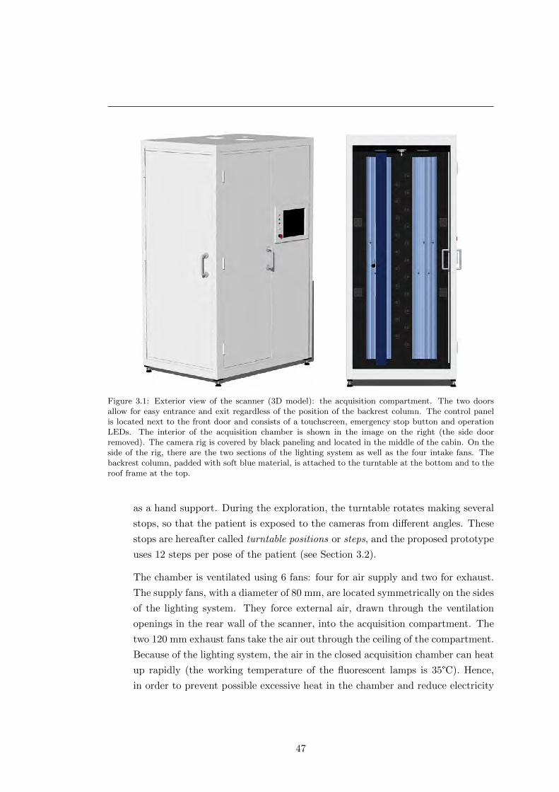
Figure 3.1: Exterior view of the scanner (3D model): the acquisition compartment. The two doorsallow for easy entrance and exit regardless of the position of the backrest column. The control panelis located next to the front door and consists of a touchscreen, emergency stop button and operationLEDs. The interior of the acquisition chamber is shown in the image on the right (the side doorremoved). The camera rig is covered by black paneling and located in the middle of the cabin. On theside of the rig, there are the two sections of the lighting system as well as the four intake fans. Thebackrest column, padded with soft blue material, is attached to the turntable at the bottom and to theroof frame at the top.
as a hand support. During the exploration, the turntable rotates making several
stops, so that the patient is exposed to the cameras from different angles. These
stops are hereafter called turntable positions or steps, and the proposed prototype
uses 12 steps per pose of the patient (see Section 3.2).
The chamber is ventilated using 6 fans: four for air supply and two for exhaust.
The supply fans, with a diameter of 80 mm, are located symmetrically on the sides
of the lighting system. They force external air, drawn through the ventilation
openings in the rear wall of the scanner, into the acquisition compartment. The
two 120 mm exhaust fans take the air out through the ceiling of the compartment.
Because of the lighting system, the air in the closed acquisition chamber can heat
up rapidly (the working temperature of the fluorescent lamps is 35°C). Hence,
in order to prevent possible excessive heat in the chamber and reduce electricity
47
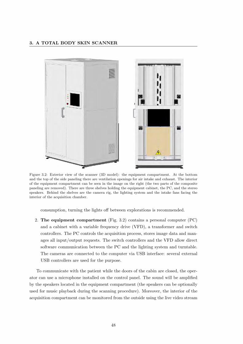
3. A TOTAL BODY SKIN SCANNER
Figure 3.2: Exterior view of the scanner (3D model): the equipment compartment. At the bottomand the top of the side paneling there are ventilation openings for air intake and exhaust. The interiorof the equipment compartment can be seen in the image on the right (the two parts of the compositepaneling are removed). There are three shelves holding the equipment cabinet, the PC, and the stereospeakers. Behind the shelves are the camera rig, the lighting system and the intake fans facing theinterior of the acquisition chamber.
consumption, turning the lights off between explorations is recommended.
2. The equipment compartment (Fig. 3.2) contains a personal computer (PC)
and a cabinet with a variable frequency drive (VFD), a transformer and switch
controllers. The PC controls the acquisition process, stores image data and man-
ages all input/output requests. The switch controllers and the VFD allow direct
software communication between the PC and the lighting system and turntable.
The cameras are connected to the computer via USB interface: several external
USB controllers are used for the purpose.
To communicate with the patient while the doors of the cabin are closed, the oper-
ator can use a microphone installed on the control panel. The sound will be amplified
by the speakers located in the equipment compartment (the speakers can be optionally
used for music playback during the scanning procedure). Moreover, the interior of the
acquisition compartment can be monitored from the outside using the live video stream
48
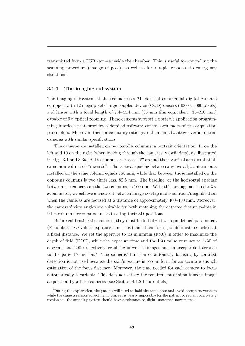
transmitted from a USB camera inside the chamber. This is useful for controlling the
scanning procedure (change of pose), as well as for a rapid response to emergency
situations.
3.1.1 The imaging subsystem
The imaging subsystem of the scanner uses 21 identical commercial digital cameras
equipped with 12 mega-pixel charge-coupled device (CCD) sensors (4000×3000 pixels)
and lenses with a focal length of 7.4–44.4 mm (35 mm film equivalent: 35–210 mm)
capable of 6× optical zooming. These cameras support a portable application program-
ming interface that provides a detailed software control over most of the acquisition
parameters. Moreover, their price-quality ratio gives them an advantage over industrial
cameras with similar specifications.
The cameras are installed on two parallel columns in portrait orientation: 11 on the
left and 10 on the right (when looking through the cameras’ viewfinders), as illustrated
in Figs. 3.1 and 3.3a. Both columns are rotated 5° around their vertical axes, so that all
cameras are directed “inwards”. The vertical spacing between any two adjacent cameras
installed on the same column equals 165 mm, while that between those installed on the
opposing columns is two times less, 82.5 mm. The baseline, or the horizontal spacing
between the cameras on the two columns, is 100 mm. With this arrangement and a 3×zoom factor, we achieve a trade-off between image overlap and resolution/magnification
when the cameras are focused at a distance of approximately 400–450 mm. Moreover,
the cameras’ view angles are suitable for both matching the detected feature points in
inter-column stereo pairs and extracting their 3D positions.
Before calibrating the cameras, they must be initialized with predefined parameters
(F-number, ISO value, exposure time, etc.) and their focus points must be locked at
a fixed distance. We set the aperture to its minimum (F8.0) in order to maximize the
depth of field (DOF), while the exposure time and the ISO value were set to 1/30 of
a second and 200 respectively, resulting in well-lit images and an acceptable tolerance
to the patient’s motion.2 The cameras’ function of automatic focusing by contrast
detection is not used because the skin’s texture is too uniform for an accurate enough
estimation of the focus distance. Moreover, the time needed for each camera to focus
automatically is variable. This does not satisfy the requirement of simultaneous image
acquisition by all the cameras (see Section 4.1.2.1 for details).
2During the exploration, the patient will need to hold the same pose and avoid abrupt movementswhile the camera sensors collect light. Since it is nearly impossible for the patient to remain completelymotionless, the scanning system should have a tolerance to slight, unwanted movements.
49
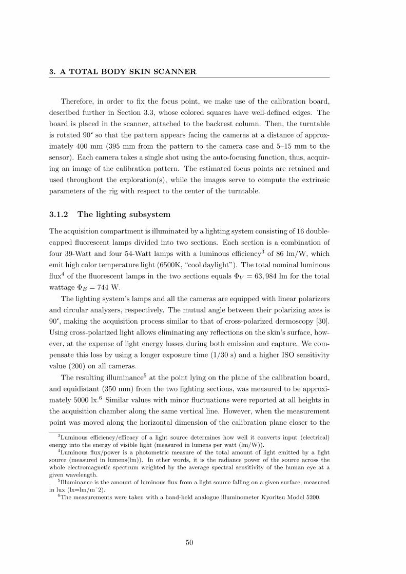
3. A TOTAL BODY SKIN SCANNER
Therefore, in order to fix the focus point, we make use of the calibration board,
described further in Section 3.3, whose colored squares have well-defined edges. The
board is placed in the scanner, attached to the backrest column. Then, the turntable
is rotated 90° so that the pattern appears facing the cameras at a distance of approx-
imately 400 mm (395 mm from the pattern to the camera case and 5–15 mm to the
sensor). Each camera takes a single shot using the auto-focusing function, thus, acquir-
ing an image of the calibration pattern. The estimated focus points are retained and
used throughout the exploration(s), while the images serve to compute the extrinsic
parameters of the rig with respect to the center of the turntable.
3.1.2 The lighting subsystem
The acquisition compartment is illuminated by a lighting system consisting of 16 double-
capped fluorescent lamps divided into two sections. Each section is a combination of
four 39-Watt and four 54-Watt lamps with a luminous efficiency3 of 86 lm/W, which
emit high color temperature light (6500K, “cool daylight”). The total nominal luminous
flux4 of the fluorescent lamps in the two sections equals ΦV = 63, 984 lm for the total
wattage ΦE = 744 W.
The lighting system’s lamps and all the cameras are equipped with linear polarizers
and circular analyzers, respectively. The mutual angle between their polarizing axes is
90°, making the acquisition process similar to that of cross-polarized dermoscopy [30].
Using cross-polarized light allows eliminating any reflections on the skin’s surface, how-
ever, at the expense of light energy losses during both emission and capture. We com-
pensate this loss by using a longer exposure time (1/30 s) and a higher ISO sensitivity
value (200) on all cameras.
The resulting illuminance5 at the point lying on the plane of the calibration board,
and equidistant (350 mm) from the two lighting sections, was measured to be approxi-
mately 5000 lx.6 Similar values with minor fluctuations were reported at all heights in
the acquisition chamber along the same vertical line. However, when the measurement
point was moved along the horizontal dimension of the calibration plane closer to the
3Luminous efficiency/efficacy of a light source determines how well it converts input (electrical)energy into the energy of visible light (measured in lumens per watt (lm/W)).
4Luminous flux/power is a photometric measure of the total amount of light emitted by a lightsource (measured in lumens(lm)). In other words, it is the radiance power of the source across thewhole electromagnetic spectrum weighted by the average spectral sensitivity of the human eye at agiven wavelength.
5Illuminance is the amount of luminous flux from a light source falling on a given surface, measuredin lux (lx=lm/mˆ2).
6The measurements were taken with a hand-held analogue illuminometer Kyoritsu Model 5200.
50

center of light ray concentration of the lighting system sections, the obtained illumi-
nance values reached as much as 7000 lx. These levels of illuminance are adequate to
uniformly light the skin surface of the patient at the focusing distance of the camera
rig and account for light losses during the image’s capture. For comparison, the recom-
mended level of illuminance for the performance of visual tasks of low contrast or very
small size over a prolonged period (inspection tasks, very difficult assembly or jewelery
manufacturing) is 2000–5000 lx [385].
According to [386], fluorescent light sources with similar characteristics belong to
the Risk Group 0 (RG0, “exempt from risk”) of photo-biological hazard. Moreover,
the effects of short-term exposure to ultraviolet radiation emitted by a fluorescent light
source are thought to be negligible. Similarly, there is no evidence that blue light from
artificial lighting belonging to RG0 would have an impact on the retina greater than
that of sunlight. Therefore, as the sole precaution during the exploration, the patient is
advised to either avoid looking directly at the light source or have his/her eyes closed.
3.2 The scanning procedure
Once the focus points are fixed and the cameras calibrated (see Section 3.3), the image
acquisition procedure can be started. In order to photograph a minimum of 85% of the
skin’s surface, the patient needs to assume two poses:
� Pose 1: face the backrest column with the hands down at the sides (Fig. 3.3b).
Used to scan the posterior region of the body, the shoulders, the arms and the
back of the hands.
� Pose 2: back to the column, grasping the horizontal bar behind with both hands
(Fig. 3.3c). Exposes the anterior region of the body, the face and the sides of the
trunk to the cameras .
To begin, the patient assumes pose 1. The turntable rotates 180 degrees counter-
clockwise making stops for the cameras to acquire images at the following 11 angles or
positions: 15°, 30°, 45°, 60°, 80°, 100°, 120°, 135°, 150°, 165° and 180° (see Fig. 3.4).
In total, there are 12 positions at which the images are acquired, starting with step
0, when the turntable is in the initial state. Note that in the range of the first and
the last 4 positions, the turntable makes 15-degree rotations each step, while at the
four middle positions it rotates 20°. This is done to increase the overlap between the
images acquired when the body (shoulders) is closer to the cameras, and hence, the
51
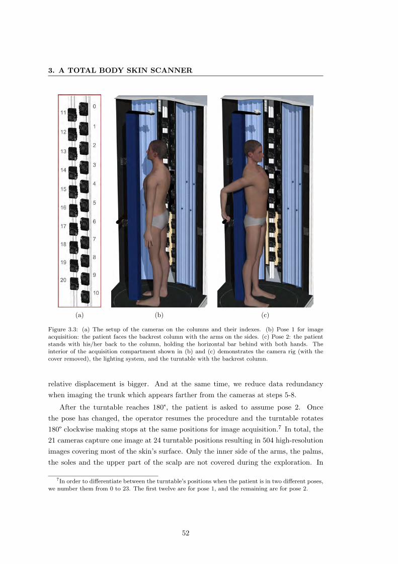
3. A TOTAL BODY SKIN SCANNER
(a) (b) (c)
Figure 3.3: (a) The setup of the cameras on the columns and their indexes. (b) Pose 1 for imageacquisition: the patient faces the backrest column with the arms on the sides. (c) Pose 2: the patientstands with his/her back to the column, holding the horizontal bar behind with both hands. Theinterior of the acquisition compartment shown in (b) and (c) demonstrates the camera rig (with thecover removed), the lighting system, and the turntable with the backrest column.
relative displacement is bigger. And at the same time, we reduce data redundancy
when imaging the trunk which appears farther from the cameras at steps 5-8.
After the turntable reaches 180°, the patient is asked to assume pose 2. Once
the pose has changed, the operator resumes the procedure and the turntable rotates
180° clockwise making stops at the same positions for image acquisition.7 In total, the
21 cameras capture one image at 24 turntable positions resulting in 504 high-resolution
images covering most of the skin’s surface. Only the inner side of the arms, the palms,
the soles and the upper part of the scalp are not covered during the exploration. In
7In order to differentiate between the turntable’s positions when the patient is in two different poses,we number them from 0 to 23. The first twelve are for pose 1, and the remaining are for pose 2.
52
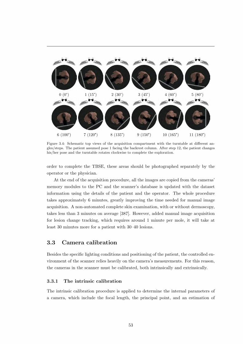
0 (0°) 1 (15°) 2 (30°) 3 (45°) 4 (60°) 5 (80°)
6 (100°) 7 (120°) 8 (135°) 9 (150°) 10 (165°) 11 (180°)
Figure 3.4: Schematic top views of the acquisition compartment with the turntable at different an-gles/steps. The patient assumed pose 1 facing the backrest column. After step 12, the patient changeshis/her pose and the turntable rotates clockwise to complete the exploration.
order to complete the TBSE, these areas should be photographed separately by the
operator or the physician.
At the end of the acquisition procedure, all the images are copied from the cameras’
memory modules to the PC and the scanner’s database is updated with the dataset
information using the details of the patient and the operator. The whole procedure
takes approximately 6 minutes, greatly improving the time needed for manual image
acquisition. A non-automated complete skin examination, with or without dermoscopy,
takes less than 3 minutes on average [387]. However, added manual image acquisition
for lesion change tracking, which requires around 1 minute per mole, it will take at
least 30 minutes more for a patient with 30–40 lesions.
3.3 Camera calibration
Besides the specific lighting conditions and positioning of the patient, the controlled en-
vironment of the scanner relies heavily on the camera’s measurements. For this reason,
the cameras in the scanner must be calibrated, both intrinsically and extrinsically.
3.3.1 The intrinsic calibration
The intrinsic calibration procedure is applied to determine the internal parameters of
a camera, which include the focal length, the principal point, and an estimation of
53

3. A TOTAL BODY SKIN SCANNER
the lens distortion. These parameters need to be estimated not only to obtain the
exact characteristics of a camera, but also to make use of the epipolar geometry (see
Appendix A.2) when one or two cameras are installed in a stereo rig. In brief, the focal
length is the distance between the focal point of the lens and the image plane (the
sensor of the camera). The projection of the focal point onto the image plane along
the optical axis8 defines the principal point. Finally, there are several types of lens
distortion, such as radial, tangential and “thin prism”, which can be approximated by
means of different models. These models are normally represented using a system of
parametric equations, which reduce the description of distortion to several parameters.
Detailed information on the intrinsic camera parameters and a variety of methods for
their estimation can be found in [388,389].
Despite the fact that all the cameras employed in the scanner are of the same
model, the intrinsic calibration we obtain for one cannot be applied to all. This is
due to distinctions in the acquired parameters which are normally the result of lens
imperfections or differences in the mechanical components. These distinctions lead
to considerable inaccuracies in the epipolar geometry of the camera rig, which is an
important part of the lesion mapping pipeline (see Section 4).
Therefore, each camera had to be calibrated individually. For that purpose, we used
a black-and-white calibration checkerboard containing 19× 27 squares of 9.5× 9.5 mm
and the Camera Calibration Toolbox for Matlabr [390]. According to the pinhole
camera model [388], the projection of a point Q = (X,Y, Z)T , given in the camera’s
reference frame, to the image plane is:
q =
[f XZ + px
f YZ + py
], (3.1)
where f is the focal length of the camera, and (px, py)T are the coordinates of the
principal point (all expressed in metrics).
The goal of the camera calibration procedure is to find the transformation matrix
K, so that: [q
1
]= K[I|0]
[Q
1
]. (3.2)
In this equation, I is a 3 × 3 identity matrix, 0 is a 3 × 1 vector of zeros, and the
resulting point q is expressed in homogeneous coordinates. The matrix K is called the
8The optical axis is the line passing through the center(s) of curvature of the lens or an opticalsystem. This axis normally coincides with the symmetry axis of the lens(es).
54
intrinsic camera calibration matrix and has the following form:
K =
f 0 px
0 f py
0 0 1
. (3.3)
Eq. 3.2 assumes that point Q is expressed in the coordinate system of the camera.
When the point(s) in space Q are expressed in terms of a different coordinate system
(the world coordinate frame), Eq. 3.2 is generalized to include the camera’s orientation
and position with respect to that system:[q
1
]= K[R|t]
[Q
1
]. (3.4)
R is the rotation matrix and t is the translation vector, which together represent the
extrinsic parameters of the camera.
When we work with CCD cameras, it is convenient to establish direct metric-to-
pixel correspondences. Thus, to obtain a point on the image plane expressed in pixel
units, we can modify K in the following way:
K′ =
mx 0 0
0 my 0
0 0 1
· K =
αx 0 x0
0 αy y0
0 0 1
. (3.5)
In this representation, mx and my are the pixel dimensions in the horizontal and vertical
directions respectively, αx = fmx and αy = fmy represent the focal length of the
camera in pixel units, and (x0, y0) are the coordinates of the principal point, also in
pixels. A more generic version of the calibration matrix K′ includes a skew parameter
for non-rectangular pixels K′1,2 = s, however, it is seldom used, and is normally equal
to zero.
However, the simplest pinhole model described above does not provide a description
of the lens distortion, and hence, cannot be accurately applied to real cameras. In order
to add distortion to the pinhole model, we need to start at the very beginning as lens
distortion occurs during the initial projection of the world point to the image plane.
Assuming a normalized projection of point Q onto the image plane (f = 1), and that
the origin of the camera coordinates coincides with the principal point (px = py = 0),
55
3. A TOTAL BODY SKIN SCANNER
we obtain
qn =
[qnx
qny
]=
[XZYZ
]. (3.6)
Having a distortion model, we can apply it directly to the normalized image coordinates
and obtain the distorted point qd. The distortion model implemented in [390] combines
the radial and tangential components in the following way:
qd = drqn + dt = (1 + k1r2 + k2r
4)
[qnx
qny
]+
[2k3 · qnxqny + k4(r2 + 2q2
nx)
2k4 · qnxqny + k3(r2 + 2q2ny)
], (3.7)
where r2 = q2nx + q2
ny , and {k1, k2} and {k3, k4} are the coefficients for the radial and
the tangential components, respectively.
Now, in order to obtain the normalized distorted point qd in pixel units, it has to
be denormalized and transformed accordingly using the calibration matrix K′:
qp = K′qd. (3.8)
Once the point correspondences Q 7→ qp are known, the calibration using the tool-
box is performed in two steps [390]: the initialization and the nonlinear optimization.
The initialization provides a closed-form solution to compute the calibration parame-
ters based on the vanishing points and using the pinhole model without lens distortion.
During the nonlinear optimization step, the total reprojection error is iteratively min-
imized (in the least-squares sense) over all the calibration parameters by means of the
gradient descent algorithm. As the toolbox also computes the extrinsic parameters of
the cameras with respect to the calibration plane, there will be 8 + 6n parameters
to estimate: 8 intrinsic (αx, αy, (px; py), {k1, k2, k3, k4}) and 6n extrinsic (3 angles of
rotation and 3 displacements, where n is the number of pattern images).
Table 3.1 shows the parameters obtained after calibrating all the cameras in the
rig. As can be seen, there is a considerable discrepancy between the estimated lo-
cations of the principal points for different cameras. In a perfect camera assembly,
we would expect the principal point to be in the geometrical center of the sensor at
the pixel (1500; 2000). However, its mean location for the 21 calibrated cameras is
at (1495.60; 1972.28), with a standard deviation of 94.6 and 30.96 pixels for the hor-
izontal and the vertical coordinates, respectively. The error, or the uncertainty, of
the estimated principal points for all the cameras has a mean value of 2.92 pixels for
the horizontal and 3.15 for the vertical coordinate. This is a solid result, especially
considering the high image resolution of 3000× 4000 pixels.
56
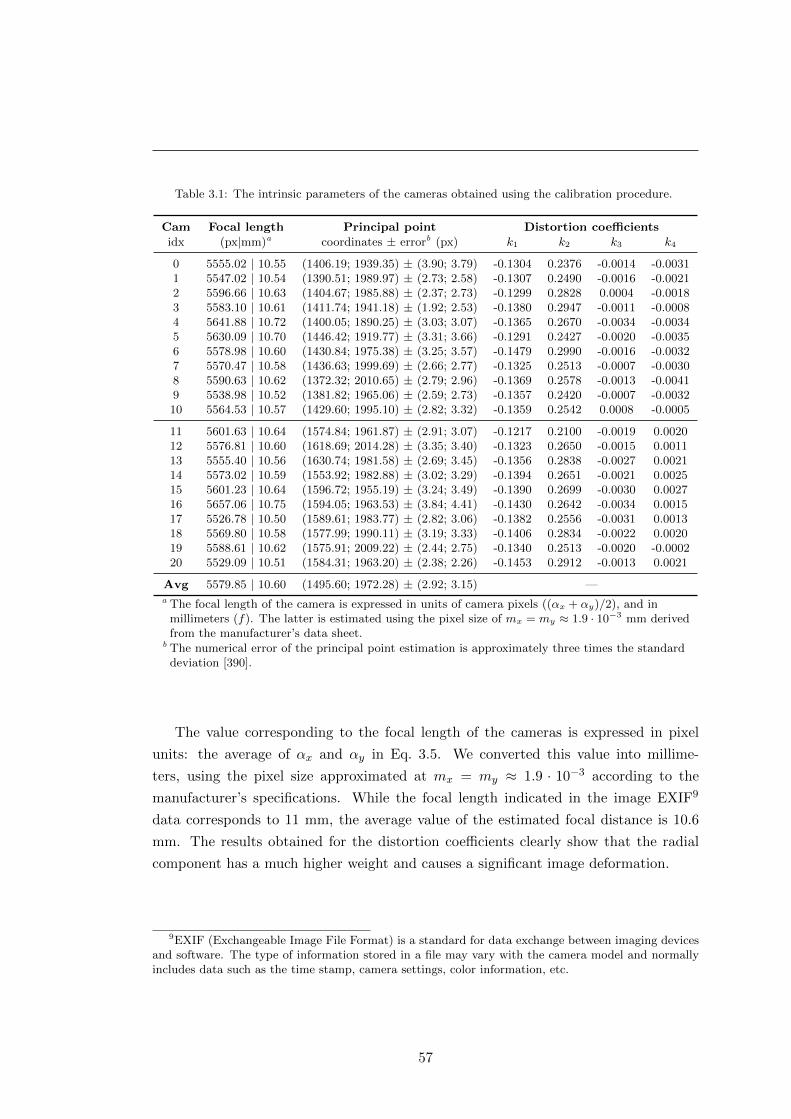
Table 3.1: The intrinsic parameters of the cameras obtained using the calibration procedure.
Cam Focal length Principal point Distortion coefficients
idx (px|mm)a coordinates ± errorb (px) k1 k2 k3 k4
0 5555.02 | 10.55 (1406.19; 1939.35) ± (3.90; 3.79) -0.1304 0.2376 -0.0014 -0.00311 5547.02 | 10.54 (1390.51; 1989.97) ± (2.73; 2.58) -0.1307 0.2490 -0.0016 -0.00212 5596.66 | 10.63 (1404.67; 1985.88) ± (2.37; 2.73) -0.1299 0.2828 0.0004 -0.00183 5583.10 | 10.61 (1411.74; 1941.18) ± (1.92; 2.53) -0.1380 0.2947 -0.0011 -0.00084 5641.88 | 10.72 (1400.05; 1890.25) ± (3.03; 3.07) -0.1365 0.2670 -0.0034 -0.00345 5630.09 | 10.70 (1446.42; 1919.77) ± (3.31; 3.66) -0.1291 0.2427 -0.0020 -0.00356 5578.98 | 10.60 (1430.84; 1975.38) ± (3.25; 3.57) -0.1479 0.2990 -0.0016 -0.00327 5570.47 | 10.58 (1436.63; 1999.69) ± (2.66; 2.77) -0.1325 0.2513 -0.0007 -0.00308 5590.63 | 10.62 (1372.32; 2010.65) ± (2.79; 2.96) -0.1369 0.2578 -0.0013 -0.00419 5538.98 | 10.52 (1381.82; 1965.06) ± (2.59; 2.73) -0.1357 0.2420 -0.0007 -0.003210 5564.53 | 10.57 (1429.60; 1995.10) ± (2.82; 3.32) -0.1359 0.2542 0.0008 -0.0005
11 5601.63 | 10.64 (1574.84; 1961.87) ± (2.91; 3.07) -0.1217 0.2100 -0.0019 0.002012 5576.81 | 10.60 (1618.69; 2014.28) ± (3.35; 3.40) -0.1323 0.2650 -0.0015 0.001113 5555.40 | 10.56 (1630.74; 1981.58) ± (2.69; 3.45) -0.1356 0.2838 -0.0027 0.002114 5573.02 | 10.59 (1553.92; 1982.88) ± (3.02; 3.29) -0.1394 0.2651 -0.0021 0.002515 5601.23 | 10.64 (1596.72; 1955.19) ± (3.24; 3.49) -0.1390 0.2699 -0.0030 0.002716 5657.06 | 10.75 (1594.05; 1963.53) ± (3.84; 4.41) -0.1430 0.2642 -0.0034 0.001517 5526.78 | 10.50 (1589.61; 1983.77) ± (2.82; 3.06) -0.1382 0.2556 -0.0031 0.001318 5569.80 | 10.58 (1577.99; 1990.11) ± (3.19; 3.33) -0.1406 0.2834 -0.0022 0.002019 5588.61 | 10.62 (1575.91; 2009.22) ± (2.44; 2.75) -0.1340 0.2513 -0.0020 -0.000220 5529.09 | 10.51 (1584.31; 1963.20) ± (2.38; 2.26) -0.1453 0.2912 -0.0013 0.0021
Avg 5579.85 | 10.60 (1495.60; 1972.28) ± (2.92; 3.15) —a The focal length of the camera is expressed in units of camera pixels ((αx + αy)/2), and in
millimeters (f). The latter is estimated using the pixel size of mx = my ≈ 1.9 · 10−3 mm derivedfrom the manufacturer’s data sheet.
b The numerical error of the principal point estimation is approximately three times the standarddeviation [390].
The value corresponding to the focal length of the cameras is expressed in pixel
units: the average of αx and αy in Eq. 3.5. We converted this value into millime-
ters, using the pixel size approximated at mx = my ≈ 1.9 · 10−3 according to the
manufacturer’s specifications. While the focal length indicated in the image EXIF9
data corresponds to 11 mm, the average value of the estimated focal distance is 10.6
mm. The results obtained for the distortion coefficients clearly show that the radial
component has a much higher weight and causes a significant image deformation.
9EXIF (Exchangeable Image File Format) is a standard for data exchange between imaging devicesand software. The type of information stored in a file may vary with the camera model and normallyincludes data such as the time stamp, camera settings, color information, etc.
57
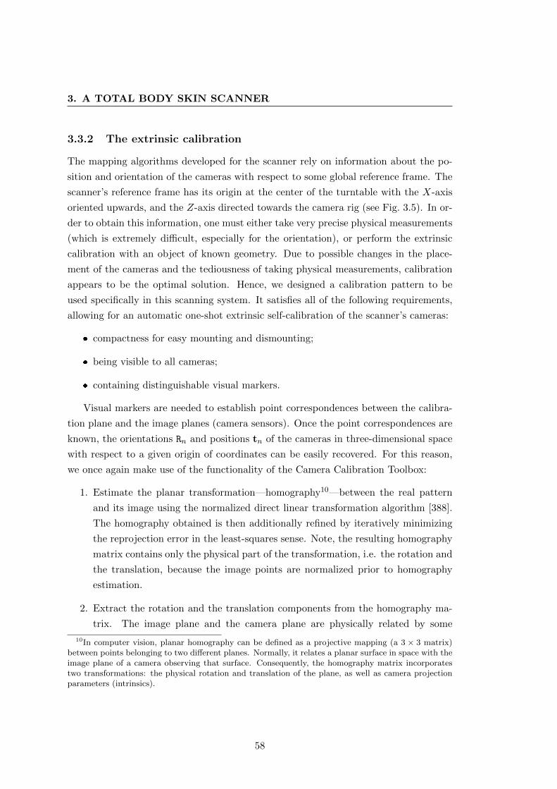
3. A TOTAL BODY SKIN SCANNER
3.3.2 The extrinsic calibration
The mapping algorithms developed for the scanner rely on information about the po-
sition and orientation of the cameras with respect to some global reference frame. The
scanner’s reference frame has its origin at the center of the turntable with the X-axis
oriented upwards, and the Z-axis directed towards the camera rig (see Fig. 3.5). In or-
der to obtain this information, one must either take very precise physical measurements
(which is extremely difficult, especially for the orientation), or perform the extrinsic
calibration with an object of known geometry. Due to possible changes in the place-
ment of the cameras and the tediousness of taking physical measurements, calibration
appears to be the optimal solution. Hence, we designed a calibration pattern to be
used specifically in this scanning system. It satisfies all of the following requirements,
allowing for an automatic one-shot extrinsic self-calibration of the scanner’s cameras:
� compactness for easy mounting and dismounting;
� being visible to all cameras;
� containing distinguishable visual markers.
Visual markers are needed to establish point correspondences between the calibra-
tion plane and the image planes (camera sensors). Once the point correspondences are
known, the orientations Rn and positions tn of the cameras in three-dimensional space
with respect to a given origin of coordinates can be easily recovered. For this reason,
we once again make use of the functionality of the Camera Calibration Toolbox:
1. Estimate the planar transformation—homography10—between the real pattern
and its image using the normalized direct linear transformation algorithm [388].
The homography obtained is then additionally refined by iteratively minimizing
the reprojection error in the least-squares sense. Note, the resulting homography
matrix contains only the physical part of the transformation, i.e. the rotation and
the translation, because the image points are normalized prior to homography
estimation.
2. Extract the rotation and the translation components from the homography ma-
trix. The image plane and the camera plane are physically related by some
10In computer vision, planar homography can be defined as a projective mapping (a 3 × 3 matrix)between points belonging to two different planes. Normally, it relates a planar surface in space with theimage plane of a camera observing that surface. Consequently, the homography matrix incorporatestwo transformations: the physical rotation and translation of the plane, as well as camera projectionparameters (intrinsics).
58

Figure 3.5: Schematic representation of the coordinate systems used in the scanner. The origin of theworld coordinate system Ow is in the center of the turntable. Ob and Oc1 ..Oc21 are the coordinateorigins of the calibration board and the cameras, respectively.
rotation R and some translation t. Hence, we can rewrite Eq. 3.4 to represent
the homography between the point on the plane (Z = 0) and a normalized image
plane point:
[qn
1
]=[R|t] [Q
1
]=[r1 r2 r3 t
]X
Y
0
1
=[r1 r2 t
]XY1
. (3.9)
Therefore, qnxqny1
= sH
XY1
, (3.10)
where H is the homography matrix defined up to a scale factor s due to universal
scale ambiguity (s is decoupled from H). From this last equation, we can directly
deduce the translation vector t and the rotation components r1 and r2 which
must be normalized previously. Finally, the third rotation vector can be found
using the orthogonality property: r3 = r1 × r2.
3.3.2.1 The calibration board
The calibration pattern is based on a colored checkerboard with squares of 10 × 10
mm. In this pattern, vertices common to at least four adjacent squares represent
59

3. A TOTAL BODY SKIN SCANNER
marker points, which are also referred to as corners. Each corner can be made unique
and distinguishable by means of the colors of the squares and additional symbolic
information. In order to minimize the number of distinct colors used in this encoding
and to maximize the number of codes they provide, the colors are distributed in the
pattern according to what we define as the abacus encoding scheme. The name suggests
an analogy with abacus beads alternately slid along adjacent wires in order to create a
number or, in this case, a pattern.
The idea of the scheme is the following: given n (n ∈ Z, n > 0) uniquely col-
ored squares and one distinguishable separator square, we can build a pattern X =
[x1 · · ·xk · · ·xn+1]T , where x1 . . .xn+1 are row-vectors with (2n + 1) elements, while
k is the position of the middle row. This pattern will contain an n × 2n matrix C of
uniquely encoded internal corners (markers). In order to build X and obtain C, we need
to perform the following steps:
(1) Using the given squares, create a row-vector y = 〈y1, y2, . . . , y6n+1〉, where colored
squares and separators are alternated, so that there are exactly 2n − 1 squares
between any two repeating colors. Start with the separator square.
(2) Superimpose a window w of 2n+ 1 elements on vector y at position pk = 2n+ 1,
so that:
wpk = 〈ypk , ypk+1, . . . ypk+2n+1〉. (3.11)
(3) Determine the index of the middle row (xk) of pattern X and assign the selected
window wpk to it:
k = d(n+ 1)/2e, (3.12)
xk = wpk , (3.13)
where d·e is the ceiling operator returning the smallest integer that is greater than
or equal to the enclosed value.
(4) The rest of the rows in X are assigned by sliding window w left or right along y:
xi = wpi = 〈ypi , ypi+1, . . . ypi+2n+1〉, (3.14)
where
pi =
{pk +m, if m ∈ 2Z + 1
pk −m, if m ∈ 2Zand m = |k − i|. (3.15)
(5) Matrix C is formed by the internal corners of pattern X. Each corner is uniquely
60
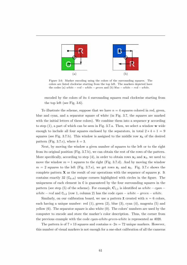
(a) (b)
Figure 3.6: Marker encoding using the colors of the surrounding squares. Thecolors are listed clockwise starting from the top left. The markers depicted havethe codes (a) white− red− white− green and (b) blue− white− red− white.
encoded by the colors of its 4 surrounding squares read clockwise starting from
the top left (see Fig. 3.6).
To illustrate the scheme, suppose that we have n = 4 squares colored in red, green,
blue and cyan, and a separator square of white (in Fig. 3.7, the squares are marked
with the initial letters of these colors). We combine them into a sequence y according
to step (1), a part of which can be seen in Fig. 3.7.a. Then, we select a window w wide
enough to include all four squares enclosed by the separators, in total 2 ∗ 4 + 1 = 9
squares (see Fig. 3.7.b). This window is assigned to the middle row xk of the desired
pattern (Fig. 3.7.c), where k = 3.
Next, by moving the window a given number of squares to the left or to the right
from its original position (Fig. 3.7.b), we can obtain the rest of the rows of the pattern.
More specifically, according to step (4), in order to obtain rows x2 and x4, we need to
move the window m = 1 squares to the right (Fig. 3.7.d). And by moving the window
m = 2 squares to the left (Fig. 3.7.e), we get rows x1 and x5. Fig. 3.7.c shows the
complete pattern X as the result of our operations with the sequence of squares y. It
contains exactly 32 (C4×8) unique corners highlighted with circles in the figure. The
uniqueness of each element in C is guaranteed by the four surrounding squares in the
pattern (see step (5) of the scheme). For example, C1,1 is identified as white− cyan−white− red and C1,2 (row 1, column 2) has the code cyan− white− green− white.
Similarly, on our calibration board, we use a pattern X created with n = 6 colors,
each having a unique number: red (1), green (2), blue (3), cyan (4), magenta (5) and
yellow (6). The separator square is also white (0). The colors’ numbers are used by the
computer to encode and store the marker’s color description. Thus, the corner from
the previous example with the code cyan-white-green-white is represented as 4020.
The pattern is of 7× 13 squares and contains n · 2n = 72 unique markers. However,
this number of visual markers is not enough for a one-shot calibration of all the cameras
61

3. A TOTAL BODY SKIN SCANNER
Figure 3.7: The abacus encoding scheme for n = 4 colors. (a) Part of the vector y = 〈y1, y2, . . . , y25〉.(b) Window w of 2 ∗ 4 + 1 = 9 squares superimposed on y at position 9. (c) Final pattern built bycombining different parts of vector y, obtained in (b), (d) and (e). The circles denote the matrix ofmarkers (corners) C4×8. (d) Window w slid one square to the right with respect to (b). (e) Window wslid two squares to the left.
because the pattern would appear in the field of view of only a few of them. There-
fore, we replicated it and tiled the copies along the vertical and horizontal dimensions,
creating a continuous periodic pattern X′. It consists of 33× 2 sub-patterns X, so that
X′i,j = X for i, j ∈ N>0, and measures 1980×250 mm. An image of this pattern acquired
by one of the cameras is shown in Fig. 3.8.
Vertically, the tiling was done so that the last row of the upper sub-pattern X′i,j is
at the same time the first row of the sub-pattern X′i+1,j directly below it. In the same
way, for the patterns tiled horizontally, the last column of sub-pattern X′i,j to the left
is the first column of X′i,j+1 to the right. Each colored square in the pattern X′ bears
a number identifying the row i and the column j of its corresponding sub-pattern X′i,j .
This ensures the uniqueness of the markers in the whole pattern. The numbers are
written inside the squares, and their colors have the same hue, but a lower intensity
as compared to the background. In this way, the numbers are easily readable and the
color integrity of the squares is sufficient.
Overall, using this calibration pattern, all that is needed is to recognize one number
and the colors of two diagonal squares in order to identify all the markers visible in the
image. This makes it a very robust system for automatic camera calibration.
62
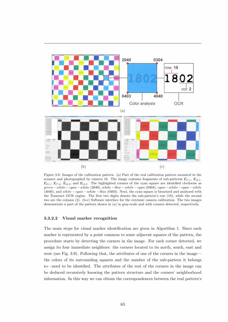
(a)
(b) (c)
Figure 3.8: Images of the calibration pattern. (a) Part of the real calibration pattern mounted in thescanner and photographed by camera 16. The image contains fragments of sub-patterns X′17,1, X′18,1,X′19,1, X′17,2, X′18,2, and X′19,2. The highlighted corners of the cyan square are identified clockwise asgreen−white− cyan−white (2040), white− blue−white− cyan (0304), cyan−white− cyan−white(4040), and white− cyan−white− blue (0403). Next, the cyan square is binarized and analyzed withthe Tesseract OCR engine. The first two digits denote the sub-pattern’s row (18), while the secondtwo are the column (2). (b-c) Software interface for the extrinsic camera calibration. The two imagesdemonstrate a part of the pattern shown in (a) in gray-scale and with corners detected, respectively.
3.3.2.2 Visual marker recognition
The main steps for visual marker identification are given in Algorithm 1. Since each
marker is represented by a point common to some adjacent squares of the pattern, the
procedure starts by detecting the corners in the image. For each corner detected, we
assign its four immediate neighbors: the corners located to its north, south, east and
west (see Fig. 3.9). Following that, the attributes of one of the corners in the image—
the colors of its surrounding squares and the number of the sub-pattern it belongs
to—need to be identified. The attributes of the rest of the corners in the image can
be deduced recursively knowing the pattern structure and the corners’ neighborhood
information. In this way we can obtain the correspondences between the real pattern’s
63

3. A TOTAL BODY SKIN SCANNER
Algorithm 1: Primary steps for visual marker identification
Data: Image of the calibration pattern I
Result: List of point correspondences pp
1 /* Corner detection */
2 /* 1. Transform I to gray scale */
3 G← colorToGrayscale(I);4 /* 2. Smooth G */
5 G← applyGaussianFilter(G);6 /* 3. Find corners in the binary image */
7 cc← detectCorners(G);
8 /* Corner identification */
9 /* 4. Assign neighbors (north, south, east and west) to each corner */
10 nn← findNeighbors(cc);11 /* 5. Recognize initial corner */
12 ppi ← identifyInitialCorner(cc,nn);13 /* 6. Identify the rest of the corners recursively */
14 pp← identifyCorners(ppi,nn)
markers and their coordinates in the images.
The steps outlined in Algorithm 1 are applied to all 21 images acquired during the
calibration phase (see Section 3.1.1). The description of each step in the algorithm is
provided below:
1. Color-to-gray-scale image conversion. The main task of the gray-scale image
conversion is to increase the contrast between the white and the colored squares
in the gray-level image. To do this we retain the lowest color intensity value for
each pixel:
Gx,y = min(Ix,y,1, Ix,y,2, Ix,y,3), (3.16)
where x, y are pixel coordinates, and I and G are the color and gray-scale images,
respectively. The white squares have higher intensities than the surrounding
colored squares in all channels, so the contrast between the resulting “white” and
“gray” areas will be significant. See Fig. 3.8b for an example of the gray-scale
conversion.
2. Smoothing the gray-scale image. After the conversion, the gray-scale image
is not going to be uniform. This is due to the image noise and the fact that
the numbers indicating the sub-pattern have lower intensities than that of their
respective squares. For these reasons, the corner detection may produce unwanted
artifact corners inside the squares. In order to smooth the non-uniform areas, the
64
image is convolved with a Gaussian filter.11 For the chosen lens magnification
factor and the distance between the calibration board and the cameras, the size
of the filter was set to 9× 9 pixels with σ = 3.
3. The corner detection is performed by means of the Harris corner detector [391].
The minimum distance between the corners found was set to 100 pixels (based
on the calibration images) and only the most stable ones in this vicinity were
retained. The sensitivity parameter of the detector was set to k = 0.2.
4. Neighbor assignment. Each marker in the real pattern has a maximum of 4
immediate orthogonal neighbors: those lying to the north, south, east and west of
the marker of interest (see Fig. 3.9a). Most of the markers have a full 4-connected
neighborhood, except for those located at the extreme corners of the calibration
pattern (2 neighbors) and those on the borders (3 neighbors).
In order to establish a link between the pattern corners detected in the images
and the real markers in the pattern, we need to determine their neighborhoods.
For that, we select the 4 points closest to each corner of interest and assess the
angles between the vectors formed by the neighbor-pairs and the axes in the
image (Fig. 3.9). The angle between the neighbor-pair vector and the vertical
axis (−→x ) conditions the north and the south neighbors, while the east and the
west neighbors are determined by the angle with the horizontal axis (−→y ). Ideally,
the vectors should coincide with the axes, but because the pattern is not strictly
fronto-parallel to the cameras, the angle will be defined within a certain range tα,
which was empirically set to 17°.
Following the example in Fig. 3.9a, point E is assigned as the eastern neighbor of
C if the angle between the vector−→CE and the −→y -axis is less than tα. Similarly,
point N is the northern neighbor of C if vector−−→CN and the −→x -axis form an angle
less than 180°− tα (compensated for the opposite directions of the vectors). The
other neighbors are assigned in the same way.
5. Corner attribute identification. In order to identify the attributes of a corner
of interest, i.e. the colors of the squares and the sub-pattern number, the regions
of interest (ROIs) corresponding to the diagonally opposite squares have to be
extracted. For that we rely on the neighborhood information obtained in the
previous step and extract the ROI containing the pattern square north-west of
11In 2-D, a circularly symmetric Gaussian filter has the form: G(x, y) = 12πσ2 e
− x2+y2
2σ2 , where σ isthe standard deviation of the Gaussian distribution.
65
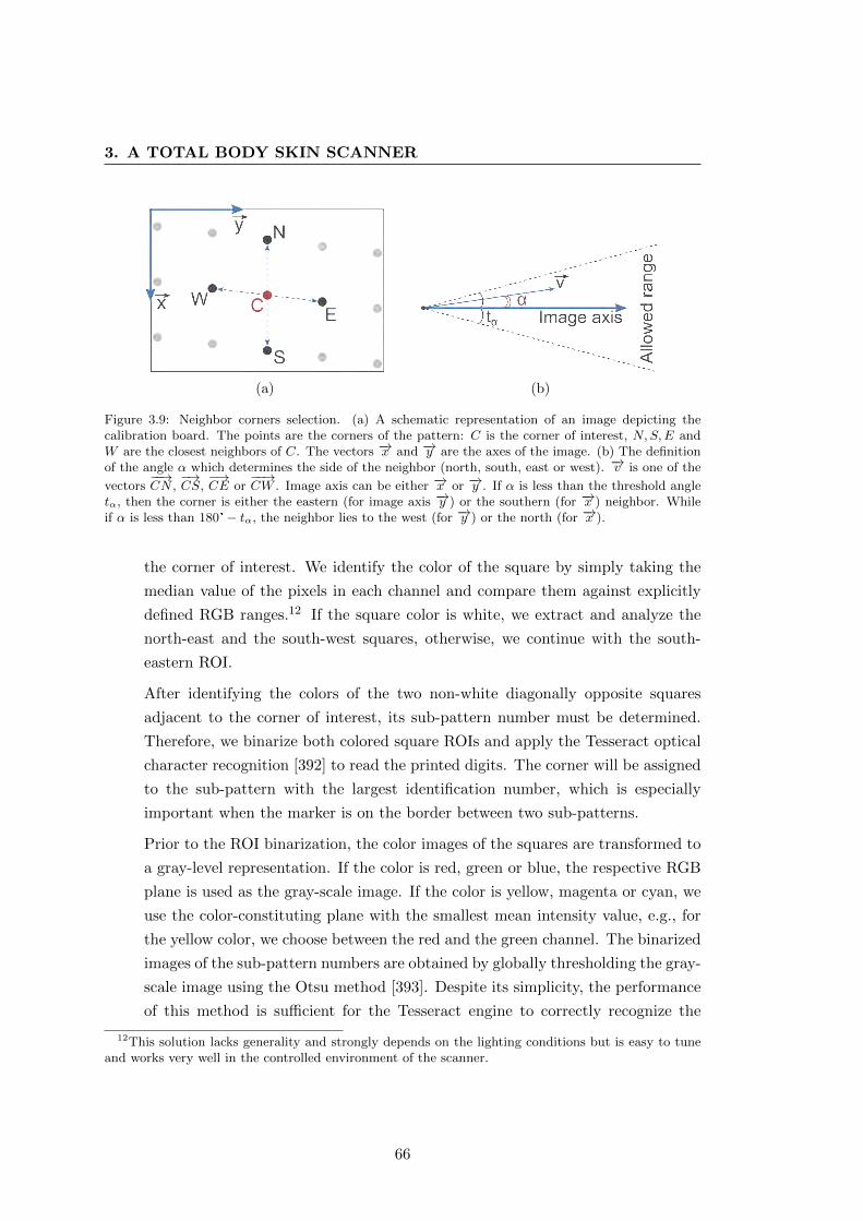
3. A TOTAL BODY SKIN SCANNER
(a) (b)
Figure 3.9: Neighbor corners selection. (a) A schematic representation of an image depicting thecalibration board. The points are the corners of the pattern: C is the corner of interest, N,S,E andW are the closest neighbors of C. The vectors −→x and −→y are the axes of the image. (b) The definitionof the angle α which determines the side of the neighbor (north, south, east or west). −→v is one of the
vectors−−→CN ,
−→CS,
−→CE or
−−→CW . Image axis can be either −→x or −→y . If α is less than the threshold angle
tα, then the corner is either the eastern (for image axis −→y ) or the southern (for −→x ) neighbor. Whileif α is less than 180°− tα, the neighbor lies to the west (for −→y ) or the north (for −→x ).
the corner of interest. We identify the color of the square by simply taking the
median value of the pixels in each channel and compare them against explicitly
defined RGB ranges.12 If the square color is white, we extract and analyze the
north-east and the south-west squares, otherwise, we continue with the south-
eastern ROI.
After identifying the colors of the two non-white diagonally opposite squares
adjacent to the corner of interest, its sub-pattern number must be determined.
Therefore, we binarize both colored square ROIs and apply the Tesseract optical
character recognition [392] to read the printed digits. The corner will be assigned
to the sub-pattern with the largest identification number, which is especially
important when the marker is on the border between two sub-patterns.
Prior to the ROI binarization, the color images of the squares are transformed to
a gray-level representation. If the color is red, green or blue, the respective RGB
plane is used as the gray-scale image. If the color is yellow, magenta or cyan, we
use the color-constituting plane with the smallest mean intensity value, e.g., for
the yellow color, we choose between the red and the green channel. The binarized
images of the sub-pattern numbers are obtained by globally thresholding the gray-
scale image using the Otsu method [393]. Despite its simplicity, the performance
of this method is sufficient for the Tesseract engine to correctly recognize the
12This solution lacks generality and strongly depends on the lighting conditions but is easy to tuneand works very well in the controlled environment of the scanner.
66
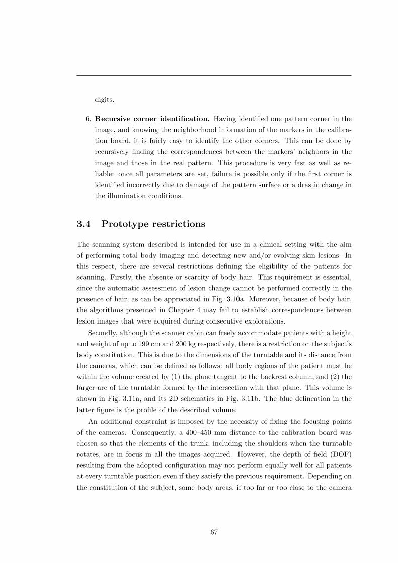
digits.
6. Recursive corner identification. Having identified one pattern corner in the
image, and knowing the neighborhood information of the markers in the calibra-
tion board, it is fairly easy to identify the other corners. This can be done by
recursively finding the correspondences between the markers’ neighbors in the
image and those in the real pattern. This procedure is very fast as well as re-
liable: once all parameters are set, failure is possible only if the first corner is
identified incorrectly due to damage of the pattern surface or a drastic change in
the illumination conditions.
3.4 Prototype restrictions
The scanning system described is intended for use in a clinical setting with the aim
of performing total body imaging and detecting new and/or evolving skin lesions. In
this respect, there are several restrictions defining the eligibility of the patients for
scanning. Firstly, the absence or scarcity of body hair. This requirement is essential,
since the automatic assessment of lesion change cannot be performed correctly in the
presence of hair, as can be appreciated in Fig. 3.10a. Moreover, because of body hair,
the algorithms presented in Chapter 4 may fail to establish correspondences between
lesion images that were acquired during consecutive explorations.
Secondly, although the scanner cabin can freely accommodate patients with a height
and weight of up to 199 cm and 200 kg respectively, there is a restriction on the subject’s
body constitution. This is due to the dimensions of the turntable and its distance from
the cameras, which can be defined as follows: all body regions of the patient must be
within the volume created by (1) the plane tangent to the backrest column, and (2) the
larger arc of the turntable formed by the intersection with that plane. This volume is
shown in Fig. 3.11a, and its 2D schematics in Fig. 3.11b. The blue delineation in the
latter figure is the profile of the described volume.
An additional constraint is imposed by the necessity of fixing the focusing points
of the cameras. Consequently, a 400–450 mm distance to the calibration board was
chosen so that the elements of the trunk, including the shoulders when the turntable
rotates, are in focus in all the images acquired. However, the depth of field (DOF)
resulting from the adopted configuration may not perform equally well for all patients
at every turntable position even if they satisfy the previous requirement. Depending on
the constitution of the subject, some body areas, if too far or too close to the camera
67
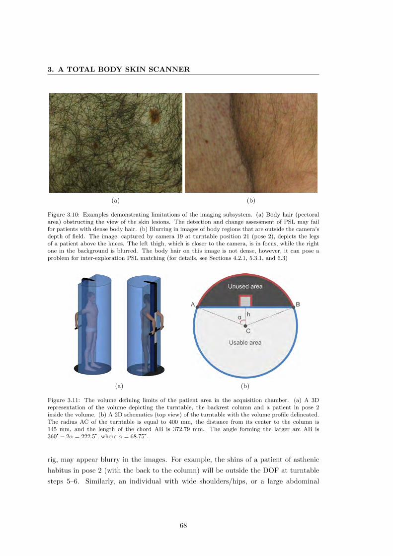
3. A TOTAL BODY SKIN SCANNER
(a) (b)
Figure 3.10: Examples demonstrating limitations of the imaging subsystem. (a) Body hair (pectoralarea) obstructing the view of the skin lesions. The detection and change assessment of PSL may failfor patients with dense body hair. (b) Blurring in images of body regions that are outside the camera’sdepth of field. The image, captured by camera 19 at turntable position 21 (pose 2), depicts the legsof a patient above the knees. The left thigh, which is closer to the camera, is in focus, while the rightone in the background is blurred. The body hair on this image is not dense, however, it can pose aproblem for inter-exploration PSL matching (for details, see Sections 4.2.1, 5.3.1, and 6.3)
(a) (b)
Figure 3.11: The volume defining limits of the patient area in the acquisition chamber. (a) A 3Drepresentation of the volume depicting the turntable, the backrest column and a patient in pose 2inside the volume. (b) A 2D schematics (top view) of the turntable with the volume profile delineated.The radius AC of the turntable is equal to 400 mm, the distance from its center to the column is145 mm, and the length of the chord AB is 372.79 mm. The angle forming the larger arc AB is360°− 2α = 222.5°, where α = 68.75°.
rig, may appear blurry in the images. For example, the shins of a patient of asthenic
habitus in pose 2 (with the back to the column) will be outside the DOF at turntable
steps 5–6. Similarly, an individual with wide shoulders/hips, or a large abdominal
68
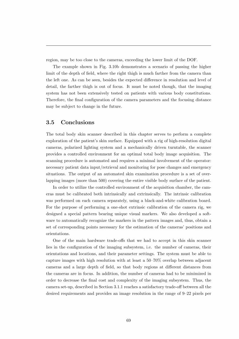
region, may be too close to the cameras, exceeding the lower limit of the DOF.
The example shown in Fig. 3.10b demonstrates a scenario of passing the higher
limit of the depth of field, where the right thigh is much farther from the camera than
the left one. As can be seen, besides the expected difference in resolution and level of
detail, the farther thigh is out of focus. It must be noted though, that the imaging
system has not been extensively tested on patients with various body constitutions.
Therefore, the final configuration of the camera parameters and the focusing distance
may be subject to change in the future.
3.5 Conclusions
The total body skin scanner described in this chapter serves to perform a complete
exploration of the patient’s skin surface. Equipped with a rig of high-resolution digital
cameras, polarized lighting system and a mechanically driven turntable, the scanner
provides a controlled environment for an optimal total body image acquisition. The
scanning procedure is automated and requires a minimal involvement of the operator:
necessary patient data input/retrieval and monitoring for pose changes and emergency
situations. The output of an automated skin examination procedure is a set of over-
lapping images (more than 500) covering the entire visible body surface of the patient.
In order to utilize the controlled environment of the acquisition chamber, the cam-
eras must be calibrated both intrinsically and extrinsically. The intrinsic calibration
was performed on each camera separately, using a black-and-white calibration board.
For the purpose of performing a one-shot extrinsic calibration of the camera rig, we
designed a special pattern bearing unique visual markers. We also developed a soft-
ware to automatically recognize the markers in the pattern images and, thus, obtain a
set of corresponding points necessary for the estimation of the cameras’ positions and
orientations.
One of the main hardware trade-offs that we had to accept in this skin scanner
lies in the configuration of the imaging subsystem, i.e. the number of cameras, their
orientations and locations, and their parameter settings. The system must be able to
capture images with high resolution with at least a 50–70% overlap between adjacent
cameras and a large depth of field, so that body regions at different distances from
the cameras are in focus. In addition, the number of cameras had to be minimized in
order to decrease the final cost and complexity of the imaging subsystem. Thus, the
camera set-up, described in Section 3.1.1 reaches a satisfactory trade-off between all the
desired requirements and provides an image resolution in the range of 9–22 pixels per
69

3. A TOTAL BODY SKIN SCANNER
millimeter (px/mm), with an average of 14 px/mm.13 Nevertheless, this setup must be
extensively tested in a real clinical setting on patients with different body constitutions,
hence, the established camera parameters and the focusing distance may be modified
to achieve a better overall performance.
In addition, there are ways to improve the image quality with respect to focusing
and image resolution, sacrificing, however, the cost of the scanner. One of them is
using either an external, active auto-focusing system based on ultrasonic sound waves
or cameras equipped with such a system. In this way, it will be possible to dynamically
define the focus point for each camera. Such a set-up can be used as far as the cameras
are able to capture images simultaneously after establishing the focusing distance.
Overall, given the characteristics of the equipment employed, the proposed scanner
set-up provides an optimal balance between the image resolution, the depth of field and
the number of cameras employed. Moreover, the mutual orientation of the two camera
columns allows for reliable interest point matching in stereo images, which, in turn,
forms the algorithmic basis for the PSL mapping proposed in the following chapter.
13This range was estimated using the PSL data of two patients of different heights and weights.Overall, the image resolution is conditioned by the distances between the cameras and the body regionin the field of view, and will vary depending on the patient’s constitution.
70
Do not “tinker” with pigmented lesions.
Stanford Cade, “Malignant Melanoma” [2]
Chapter 4
Automatic PSL change detection
The total body skin scanner presented acquires 504 high-definition skin surface
images in one exploration. This is a large amount of raw data and cannot be used “as
is” to detect changes in PSLs. In the first place, the data need to be processed so as to
segregate images of lesions which are going to be compared with the baseline. Moreover,
it is clear that many lesions will appear in more than one image, hence, it is essential
that the system identifies these lesions and keeps track of all their views. Finally, all
the PSLs detected during one exploration must be matched to those obtained in a
successive scan. Therefore, a set of image and data processing operations allowing for
such data segregation and organization, which we call mole mapping, must be applied.
Mole mapping means detecting PSLs in the images and establishing their intra- and
inter-exploration correspondences. While the former defines correspondences between
PSLs on the patient’s body and their images acquired during one exploration, the
latter links lesions between two successive scans. In other words, upon completing an
exploration, the scanner will have a set of images from different angles assigned to
each lesion detected. And after scanning the same patient again, it will automatically
determine correspondences between lesions identified in the two explorations.
4.1 Intra-exploration mole mapping
The pipeline for obtaining intra-exploration correspondences, or a mole map, consists
of the three main stages shown in Fig. 4.1. The first stage provides 2D information
about the lesions in the images, i.e. locations and dimensions. Then, this information
is passed to the next stage where groups of moles (mole sets) are acquired at each
position of the turntable. In the final stage, these sets are combined into one map.
71
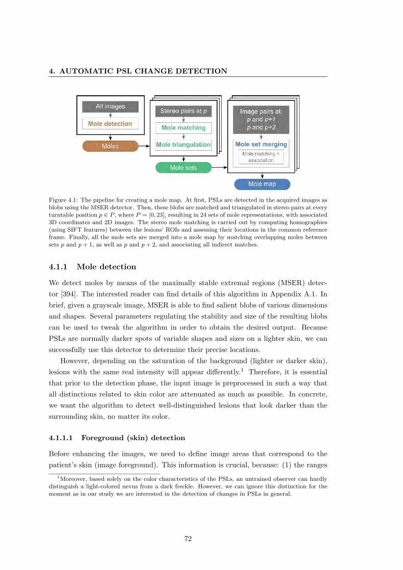
4. AUTOMATIC PSL CHANGE DETECTION
Figure 4.1: The pipeline for creating a mole map. At first, PSLs are detected in the acquired images asblobs using the MSER detector. Then, these blobs are matched and triangulated in stereo pairs at everyturntable position p ∈ P , where P = [0, 23], resulting in 24 sets of mole representations, with associated3D coordinates and 2D images. The stereo mole matching is carried out by computing homographies(using SIFT features) between the lesions’ ROIs and assessing their locations in the common referenceframe. Finally, all the mole sets are merged into a mole map by matching overlapping moles betweensets p and p+ 1, as well as p and p+ 2, and associating all indirect matches.
4.1.1 Mole detection
We detect moles by means of the maximally stable extremal regions (MSER) detec-
tor [394]. The interested reader can find details of this algorithm in Appendix A.1. In
brief, given a grayscale image, MSER is able to find salient blobs of various dimensions
and shapes. Several parameters regulating the stability and size of the resulting blobs
can be used to tweak the algorithm in order to obtain the desired output. Because
PSLs are normally darker spots of variable shapes and sizes on a lighter skin, we can
successfully use this detector to determine their precise locations.
However, depending on the saturation of the background (lighter or darker skin),
lesions with the same real intensity will appear differently.1 Therefore, it is essential
that prior to the detection phase, the input image is preprocessed in such a way that
all distinctions related to skin color are attenuated as much as possible. In concrete,
we want the algorithm to detect well-distinguished lesions that look darker than the
surrounding skin, no matter its color.
4.1.1.1 Foreground (skin) detection
Before enhancing the images, we need to define image areas that correspond to the
patient’s skin (image foreground). This information is crucial, because: (1) the ranges
1Moreover, based solely on the color characteristics of the PSLs, an untrained observer can hardlydistinguish a light-colored nevus from a dark freckle. However, we can ignore this distinction for themoment as in our study we are interested in the detection of changes in PSLs in general.
72
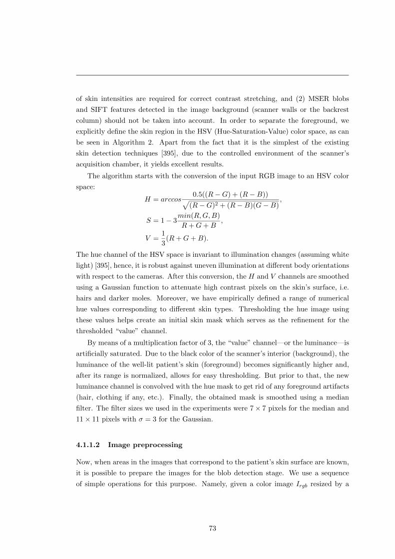
of skin intensities are required for correct contrast stretching, and (2) MSER blobs
and SIFT features detected in the image background (scanner walls or the backrest
column) should not be taken into account. In order to separate the foreground, we
explicitly define the skin region in the HSV (Hue-Saturation-Value) color space, as can
be seen in Algorithm 2. Apart from the fact that it is the simplest of the existing
skin detection techniques [395], due to the controlled environment of the scanner’s
acquisition chamber, it yields excellent results.
The algorithm starts with the conversion of the input RGB image to an HSV color
space:
H = arccos0.5((R−G) + (R−B))√
(R−G)2 + (R−B)(G−B),
S = 1− 3min(R,G,B)
R+G+B,
V =1
3(R+G+B).
The hue channel of the HSV space is invariant to illumination changes (assuming white
light) [395], hence, it is robust against uneven illumination at different body orientations
with respect to the cameras. After this conversion, the H and V channels are smoothed
using a Gaussian function to attenuate high contrast pixels on the skin’s surface, i.e.
hairs and darker moles. Moreover, we have empirically defined a range of numerical
hue values corresponding to different skin types. Thresholding the hue image using
these values helps create an initial skin mask which serves as the refinement for the
thresholded “value” channel.
By means of a multiplication factor of 3, the “value” channel—or the luminance—is
artificially saturated. Due to the black color of the scanner’s interior (background), the
luminance of the well-lit patient’s skin (foreground) becomes significantly higher and,
after its range is normalized, allows for easy thresholding. But prior to that, the new
luminance channel is convolved with the hue mask to get rid of any foreground artifacts
(hair, clothing if any, etc.). Finally, the obtained mask is smoothed using a median
filter. The filter sizes we used in the experiments were 7× 7 pixels for the median and
11× 11 pixels with σ = 3 for the Gaussian.
4.1.1.2 Image preprocessing
Now, when areas in the images that correspond to the patient’s skin surface are known,
it is possible to prepare the images for the blob detection stage. We use a sequence
of simple operations for this purpose. Namely, given a color image Irgb resized by a
73
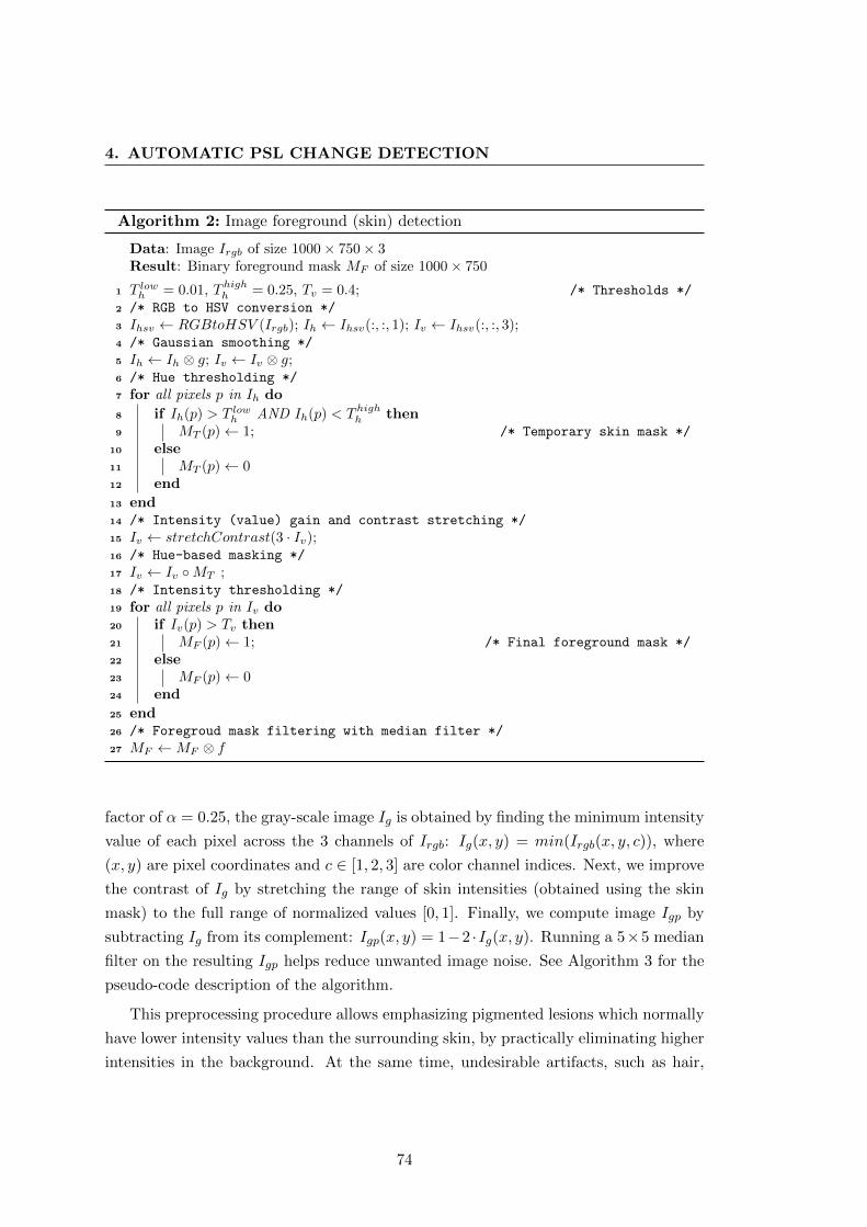
4. AUTOMATIC PSL CHANGE DETECTION
Algorithm 2: Image foreground (skin) detection
Data: Image Irgb of size 1000× 750× 3Result: Binary foreground mask MF of size 1000× 750
1 T lowh = 0.01, Thigh
h = 0.25, Tv = 0.4; /* Thresholds */
2 /* RGB to HSV conversion */
3 Ihsv ← RGBtoHSV (Irgb); Ih ← Ihsv(:, :, 1); Iv ← Ihsv(:, :, 3);4 /* Gaussian smoothing */
5 Ih ← Ih ⊗ g; Iv ← Iv ⊗ g;6 /* Hue thresholding */
7 for all pixels p in Ih do
8 if Ih(p) > T lowh AND Ih(p) < Thigh
h then9 MT (p)← 1; /* Temporary skin mask */
10 else11 MT (p)← 012 end
13 end14 /* Intensity (value) gain and contrast stretching */
15 Iv ← stretchContrast(3 · Iv);16 /* Hue-based masking */
17 Iv ← Iv ◦MT ;18 /* Intensity thresholding */
19 for all pixels p in Iv do20 if Iv(p) > Tv then21 MF (p)← 1; /* Final foreground mask */
22 else23 MF (p)← 024 end
25 end26 /* Foregroud mask filtering with median filter */
27 MF ←MF ⊗ f
factor of α = 0.25, the gray-scale image Ig is obtained by finding the minimum intensity
value of each pixel across the 3 channels of Irgb: Ig(x, y) = min(Irgb(x, y, c)), where
(x, y) are pixel coordinates and c ∈ [1, 2, 3] are color channel indices. Next, we improve
the contrast of Ig by stretching the range of skin intensities (obtained using the skin
mask) to the full range of normalized values [0, 1]. Finally, we compute image Igp by
subtracting Ig from its complement: Igp(x, y) = 1−2 ·Ig(x, y). Running a 5×5 median
filter on the resulting Igp helps reduce unwanted image noise. See Algorithm 3 for the
pseudo-code description of the algorithm.
This preprocessing procedure allows emphasizing pigmented lesions which normally
have lower intensity values than the surrounding skin, by practically eliminating higher
intensities in the background. At the same time, undesirable artifacts, such as hair,
74

Algorithm 3: Image preprocessing for mole detection
Data: RGB image Irgb of size 4000× 3000× 3Result: Processed grayscale image Igp of size 1000× 750
1 Irgb ← resize(Irgb, 0.25);2 /* Obtain grayscale image Ig */
3 for i← 1 to 1000 do4 for j ← 1 to 750 do5 Ig(i, j)← min([Irgb(i, j, 1), Irgb(i, j, 2), Irgb(i, j, 3)]);6 end
7 end8 /* Stretch image contrast using the skin intensity values */
9 Ig ← stretchContrast(Ig, skinMask);10 /* Subtract Ig from its complement */
11 Igp ← 1− 2 · Ig;12 /* Filter the result */
13 Igp ← Igp ⊗ f ;
acne and pores, are attenuated and cannot be represented as stable extremal regions
as PSLs after the preprocessing.
Running the MSER detector on the image Igp yields stable mole regions (blobs)
which are approximated by ellipses with their respective dimensions (major and minor
axes) and locations (center coordinates). Additionally, we filter these blobs based on
their size and aspect ratio. It is rather safe to assume that PSLs with the largest axis
less than Ta = 15 pixels are not going to be useful for a change analysis. Furthermore,
the natural shape of a PSL is an ellipse with a small value of flattening. Highly flattened
shapes, such as blobs produced by hair or skin folds, can be discarded by thresholding
their compression factor: the ratio between the minor and the major semi-axes. The
minimum value allowed was empirically set to Tar = 0.2.
4.1.2 Stereo-pair processing
Depending on the location, each camera in the scanner has 2 or 4 immediate neighbor
cameras, whose arrangement makes a significant vertical or horizontal overlap of their
images possible. We distinguish between vertical and diagonal camera neighbors as:
(a) adjacent cameras on the same column and (b) those belonging to different columns,
respectively. These cameras can be combined into stereo pairs, 39 in total.
The stereo image pairs acquired by these cameras can be used for matching and
subsequent triangulation of the moles detected (MSER blobs). However, stereo pairs
can be combined only using images obtained at the same turntable position p ∈ P ,
75
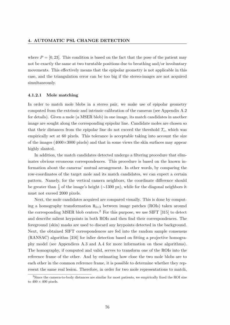
4. AUTOMATIC PSL CHANGE DETECTION
where P = [0, 23]. This condition is based on the fact that the pose of the patient may
not be exactly the same at two turntable positions due to breathing and/or involuntary
movements. This effectively means that the epipolar geometry is not applicable in this
case, and the triangulation error can be too big if the stereo-images are not acquired
simultaneously.
4.1.2.1 Mole matching
In order to match mole blobs in a stereo pair, we make use of epipolar geometry
computed from the extrinsic and intrinsic calibration of the cameras (see Appendix A.2
for details). Given a mole (a MSER blob) in one image, its match candidates in another
image are sought along the corresponding epipolar line. Candidate moles are chosen so
that their distances from the epipolar line do not exceed the threshold Te, which was
empirically set at 60 pixels. This tolerance is acceptable taking into account the size
of the images (4000×3000 pixels) and that in some views the skin surfaces may appear
highly slanted.
In addition, the match candidates detected undergo a filtering procedure that elim-
inates obvious erroneous correspondences. This procedure is based on the known in-
formation about the cameras’ mutual arrangement. In other words, by comparing the
row-coordinates of the target mole and its match candidates, we can expect a certain
pattern. Namely, for the vertical camera neighbors, the coordinate difference should
be greater than 13 of the image’s height (∼1300 px), while for the diagonal neighbors it
must not exceed 2000 pixels.
Next, the mole candidates acquired are compared visually. This is done by comput-
ing a homography transformation H3×3 between image patches (ROIs) taken around
the corresponding MSER blob centers.2 For this purpose, we use SIFT [315] to detect
and describe salient keypoints in both ROIs and then find their correspondences. The
foreground (skin) masks are used to discard any keypoints detected in the background.
Next, the obtained SIFT correspondences are fed into the random sample consensus
(RANSAC) algorithm [316] for inlier detection based on fitting a projective homogra-
phy model (see Appendices A.3 and A.4 for more information on these algorithms).
The homography, if computed and valid, serves to transform one of the ROIs into the
reference frame of the other. And by estimating how close the two mole blobs are to
each other in the common reference frame, it is possible to determine whether they rep-
resent the same real lesion. Therefore, in order for two mole representations to match,
2Since the camera-to-body distances are similar for most patients, we empirically fixed the ROI sizeto 400× 400 pixels.
76
Algorithm 4: Mole matching in a stereo pair
Data: Images I1, I2; lists of detected MSER blobs in each image m1,m2;threshold THResult: Matrix M containing index pairs of matching MSER blobs
1 /* Get epipolar match candidates */
2 cM ← getEpipolarMatches(m1,m2);3 for all candidates c in cM do4 /* Extract image ROIs around the blobs */
5 R1 ← extractROI(I1,m1); R2 = extractROI(I2,m2);6 /* Extract skin mask ROIs around the blobs */
7 B1 ← extractSkinMask(I1,m1); B2 = extractSkinMask(I2,m2);8 /* Compute homography transformation */
9 H← computeHomography(R1, R2, B1, B2);10 if H is NOT empty AND exp(abs(ln(abs(H(3, 1)) + abs(H(3, 2))))) > TH then11 /* Warp the MSER ellipse of mole2 to the ref. frame of mole 1 */
12 m2 ← warp(m2, H);13 /* Compute the distance between the two ellipses */
14 d← euclideanDistance(m1.location,m2.location);15 if d < m1.majorAxis AND d < m2.majorAxis then16 Append m1(cM(c, 1)) and m2(cM(c, 2)) to M17 end
18 end
19 end
the following condition has to be satisfied:
� The distance between the centers of the moles’ ellipses must be smaller than both
their major axes.
See Algorithm 4 for the pseudo-code of the matching procedure.
If the homography can be computed, i.e. there are enough SIFT feature matches,
its validity is verified by satisfying the condition
e|ln(|H3,1|+|H3,2|)| < TH, (4.1)
where TH = 800 is the accepted threshold. The absolute sum of the elements H3,1 and
H3,2 of the normalized homography can give an idea of how misshaped the image will be
after the transformation: the larger the value, the more the induced deformation. An
excessively misshaped image means that the transformation homography was computed
using wrong SIFT feature matches and, thus, should be discarded. By using logarithmic
and exponential functions, we can amplify the resulting value so that the threshold can
reliably cut off incorrect transformations.
77
4. AUTOMATIC PSL CHANGE DETECTION
4.1.2.2 Mole triangulation
Once the matching MSER blobs in a stereo pair have been found, we can now acquire
their locations in 3D space, i.e perform the triangulation. Knowing the intrinsic and
extrinsic parameters of the stereo rig, the reconstruction by triangulation is unambigu-
ous and straightforward. The “mid-point method” [396, 397] used for this purpose is
very simple. Although its accuracy is considered to be poor [397], it can well be applied
to obtain the 3D locations of PSLs. Firstly, because the final triangulation output is
not expected to be, nor can be, precise due to the unavoidable motion of the subject
during the exploration. And secondly, due to the linear implementation, the algorithm
is very fast, which is an important advantage when processing many points (lesions).
The interested reader can find a detailed explanation of the algorithm in Appendix A.5.
During the triangulation, we also compute normals to the local surfaces of the
lesions. To do this, a ring of 180 points is placed around the center of the mole ellipse
in one ROI. The diameter of the ring is equal to the major axis of the mole’s MSER
ellipse. Knowing the homography transformation between the two regions of interest,
the coordinates of each point in the ring can be computed in the other ROI. Then, by
triangulating these points, a three-dimensional ring surrounding the detected lesion is
obtained. The normal of the plane fit to the 3D point ring is the normal to the mole’s
surface.
Using the normal to the lesion surface, we can compute two important metrics. One
is the resolution of the image at the mole site, which shows how many pixels of the mole
ROI constitute 1 millimeter on the skin’s surface (px/mm). In order to compute this,
we need to know the distance from the camera to the PSL and its estimated diameter
in millimeters. While the former is straightforward, the latter can be obtained using
the relationship from the pinhole camera model [388]:
d
D=f
L. (4.2)
In this relationship, f is the focal length of the camera, L is the distance between the
mole and the camera, and D and d are the diameter of the mole and its projection (in
mm), respectively. Consequently, the local resolution of the image at the lesion site is
γ =d′
D, (4.3)
where d′ is the diameter of the lesion’s blob in pixels.
The second metric η is a relative quantitative measure which will serve to define
78

Figure 4.2: The projection, n, of a lesion’s normal unit vector, n, to the image plane. It is used tocompute the η-metric for best mole view selection.
the best view of a mole among the available images (at least two). In this metric, we
seek to maximize the pixel-per-millimeter resolution and, at the same time, minimize
the skew of the mole’s projection on the image plane. In other words, a camera with
the smallest η will be both close to the lesion and as perpendicular to its normal as
possible. The definition of the metric is
η =|n2|γ, (4.4)
where n is the image projection of the unit vector normal to the surface of the lesion
(see Fig. 4.2). The less perpendicular the mole’s normal is to the camera plane, the
larger the length of the projected vector. In addition, we raise the numerator to the
second power to prioritize the orientation of the mole over the image resolution.
Overall, the result of the stereo-pair processing performed at each turntable position
is a set of 3D points corresponding to the centers of the real PSLs. Each 3D point
has a local surface normal and is connected to the two ROIs of the stereo pair with
known px/mm resolutions and η-metrics. At this stage, the points representing the
same real lesion, but obtained using different stereo pairs, are not yet identified. This
identification is done at the next stage of the mole mapping pipeline—the mole set
creation.
4.1.3 Mole set creation
Once the detected PSLs are matched and triangulated across all stereo pairs, they
can be grouped into mole sets. A mole set is a totality of all detected lesions linked
79
4. AUTOMATIC PSL CHANGE DETECTION
with their 2-D views (ROIs containing MSER ellipses) and triangulations3 at a given
turntable position. Throughout the text, the elements of mole sets are referred to as
mole representations or virtual moles.
In order to create a mole set, the ellipses and triangulations of every PSL obtained
using various stereo pairs have to be linked together. For example, if MSER ellipse
number 15 in image 5 (m515) is matched to ellipse number 19 in image 6 (m6
19), which,
in turn, is linked to m1620, it means that ellipses m5
15 and m1620 must be connected as
well. Using recursive tracing, it is easy to recover all such indirect connections of
the triangulations via the lesion’s direct stereo match information. In this particular
example, when searching for all 2D views of a mole represented by m515, we will first
explore its stereo matches (m619), then the matches of the matches (m16
20), and so on,
until the total number of connected ellipses has been covered. In this way, we will
get a set of MSER ellipses (here, it will include only m515, m16
20, and m619) and their
corresponding triangulations representing one real PSL on the patient’s body.
The schematic in Fig. 4.3a demonstrates an ideal input for the tracing algorithm:
the MSER ellipses successfully matched and triangulated across the AB, AC, AD, BD
and CD stereo pairs. Had connections AB and AC not been established previously, the
recursive search would still show that the ellipses in images A, B, C and D represent
the same real PSL.
However, in certain cases, the tracing may not produce the desired results: it can
either create false connections or skip the true ones. Consequently, it is possible that
one lesion has multiple representations, and vice versa—several real PSLs can be rep-
resented as one mole.
4.1.3.1 Multiple representations of one lesion
It is possible that during stereo matching, an image pair depicting the same PSL is
not registered correctly due to an insufficient number of SIFT feature matches for
homography computation. Effectively, this will lead to a break in the recursive search,
and two or more groups of stereo triangulations may not be merged, creating several
representations of one real mole (see Fig. 4.3b for the schematic of such a scenario).
The problem during SIFT feature matching can be a result of the peculiarity of the
skin area around the lesion (e.g. lesions on skin folds or in areas with a non-uniform
3A real mole can have more than one triangulation because it appears in more than one stereo pairat the same turntable position. Although not coinciding completely due to image noise, their positionsare very close normally, hence, their average is a good approximation of the real mole’s location in 3Dspace.
80
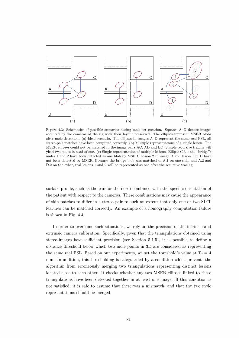
(a) (b) (c)
Figure 4.3: Schematics of possible scenarios during mole set creation. Squares A–D denote imagesacquired by the cameras of the rig with their layout preserved. The ellipses represent MSER blobsafter mole detection. (a) Ideal scenario. The ellipses in images A–D represent the same real PSL, allstereo-pair matches have been computed correctly. (b) Multiple representations of a single lesion. TheMSER ellipses could not be matched in the image pairs AC, AD and BD. Simple recursive tracing willyield two moles instead of one. (c) Single representation of multiple lesions. Ellipse C.3 is the “bridge”:moles 1 and 2 have been detected as one blob by MSER. Lesion 2 in image B and lesion 1 in D havenot been detected by MSER. Because the bridge blob was matched to A.1 on one side, and A.2 andD.2 on the other, real lesions 1 and 2 will be represented as one after the recursive tracing.
surface profile, such as the ears or the nose) combined with the specific orientation of
the patient with respect to the cameras. These combinations may cause the appearance
of skin patches to differ in a stereo pair to such an extent that only one or two SIFT
features can be matched correctly. An example of a homography computation failure
is shown in Fig. 4.4.
In order to overcome such situations, we rely on the precision of the intrinsic and
extrinsic camera calibration. Specifically, given that the triangulations obtained using
stereo-images have sufficient precision (see Section 5.1.5), it is possible to define a
distance threshold below which two mole points in 3D are considered as representing
the same real PSL. Based on our experiments, we set the threshold’s value at Td = 4
mm. In addition, this thresholding is safeguarded by a condition which prevents the
algorithm from erroneously merging two triangulations representing distinct lesions
located close to each other. It checks whether any two MSER ellipses linked to these
triangulations have been detected together in at least one image. If this condition is
not satisfied, it is safe to assume that there was a mismatch, and that the two mole
representations should be merged.
81
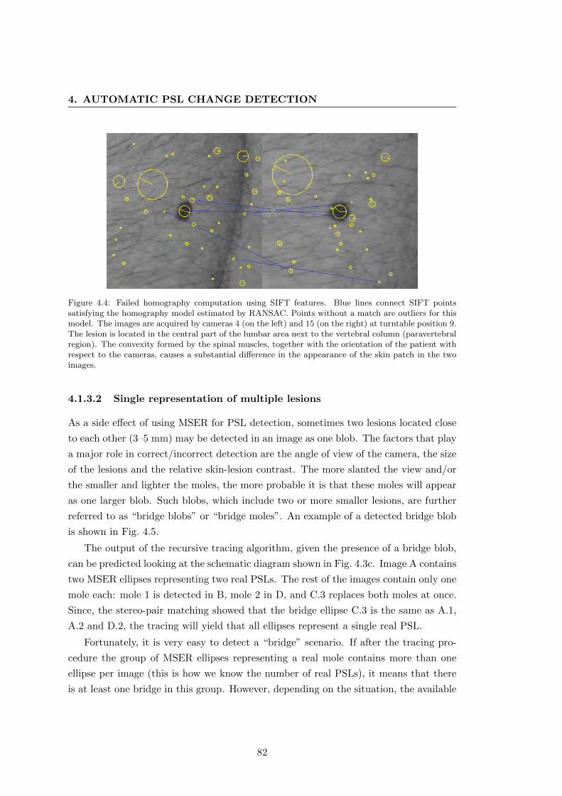
4. AUTOMATIC PSL CHANGE DETECTION
Figure 4.4: Failed homography computation using SIFT features. Blue lines connect SIFT pointssatisfying the homography model estimated by RANSAC. Points without a match are outliers for thismodel. The images are acquired by cameras 4 (on the left) and 15 (on the right) at turntable position 9.The lesion is located in the central part of the lumbar area next to the vertebral column (paravertebralregion). The convexity formed by the spinal muscles, together with the orientation of the patient withrespect to the cameras, causes a substantial difference in the appearance of the skin patch in the twoimages.
4.1.3.2 Single representation of multiple lesions
As a side effect of using MSER for PSL detection, sometimes two lesions located close
to each other (3–5 mm) may be detected in an image as one blob. The factors that play
a major role in correct/incorrect detection are the angle of view of the camera, the size
of the lesions and the relative skin-lesion contrast. The more slanted the view and/or
the smaller and lighter the moles, the more probable it is that these moles will appear
as one larger blob. Such blobs, which include two or more smaller lesions, are further
referred to as “bridge blobs” or “bridge moles”. An example of a detected bridge blob
is shown in Fig. 4.5.
The output of the recursive tracing algorithm, given the presence of a bridge blob,
can be predicted looking at the schematic diagram shown in Fig. 4.3c. Image A contains
two MSER ellipses representing two real PSLs. The rest of the images contain only one
mole each: mole 1 is detected in B, mole 2 in D, and C.3 replaces both moles at once.
Since, the stereo-pair matching showed that the bridge ellipse C.3 is the same as A.1,
A.2 and D.2, the tracing will yield that all ellipses represent a single real PSL.
Fortunately, it is very easy to detect a “bridge” scenario. If after the tracing pro-
cedure the group of MSER ellipses representing a real mole contains more than one
ellipse per image (this is how we know the number of real PSLs), it means that there
is at least one bridge in this group. However, depending on the situation, the available
82
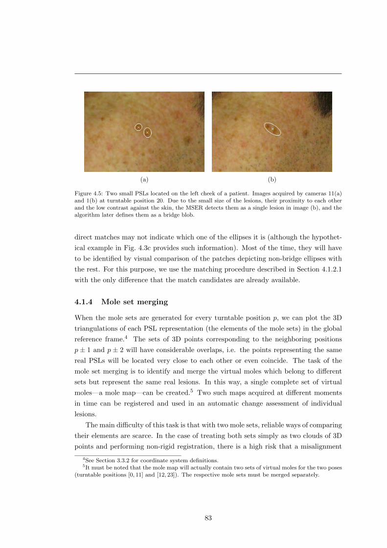
(a) (b)
Figure 4.5: Two small PSLs located on the left cheek of a patient. Images acquired by cameras 11(a)and 1(b) at turntable position 20. Due to the small size of the lesions, their proximity to each otherand the low contrast against the skin, the MSER detects them as a single lesion in image (b), and thealgorithm later defines them as a bridge blob.
direct matches may not indicate which one of the ellipses it is (although the hypothet-
ical example in Fig. 4.3c provides such information). Most of the time, they will have
to be identified by visual comparison of the patches depicting non-bridge ellipses with
the rest. For this purpose, we use the matching procedure described in Section 4.1.2.1
with the only difference that the match candidates are already available.
4.1.4 Mole set merging
When the mole sets are generated for every turntable position p, we can plot the 3D
triangulations of each PSL representation (the elements of the mole sets) in the global
reference frame.4 The sets of 3D points corresponding to the neighboring positions
p ± 1 and p ± 2 will have considerable overlaps, i.e. the points representing the same
real PSLs will be located very close to each other or even coincide. The task of the
mole set merging is to identify and merge the virtual moles which belong to different
sets but represent the same real lesions. In this way, a single complete set of virtual
moles—a mole map—can be created.5 Two such maps acquired at different moments
in time can be registered and used in an automatic change assessment of individual
lesions.
The main difficulty of this task is that with two mole sets, reliable ways of comparing
their elements are scarce. In the case of treating both sets simply as two clouds of 3D
points and performing non-rigid registration, there is a high risk that a misalignment
4See Section 3.3.2 for coordinate system definitions.5It must be noted that the mole map will actually contain two sets of virtual moles for the two poses
(turntable positions [0, 11] and [12, 23]). The respective mole sets must be merged separately.
83
4. AUTOMATIC PSL CHANGE DETECTION
will occur. The most probable scenario for that happening is the following:
� Two lesions are located next to each other on the patient’s body. One of them
was detected and triangulated only in the first mole set, while the other mole was
detected only in the second set. Using only a distance constraint with respect to
the rest of the moles, it is impossible to distinguish between the two lesions while
merging the sets, so they are very likely to be registered incorrectly.
Thus, we can use the geometrical constraint only when coupled with some additional
information such as the moles’ appearance. But the parameters of the moles’ MSER
ellipses (dimensions and orientation) are not sufficient in the case of resembling lesions
or when there is a drastic change in the viewing angle. Therefore, besides the visual in-
formation of the lesion itself, the topological information around the mole (neighboring
lesions and the skin) must be taken into account as well.
4.1.4.1 Matching moles across mole sets
In order to carry out the comparison of two virtual moles belonging to different mole
sets, taking into account both the geometrical and visual constraints, we can apply
the principle of the mole matching procedure described in Section 4.1.2.1. However, a
number of important adjustments and modifications need to be made:
1. Match candidate selection. The candidate pairs are selected based on their
distance from each other in 3D space: moles within the radius of rc = 30 mm are
chosen for visual comparison. This distance is enough to account for slight pose
shifts of the patient during the turntable rotation. Using this approach, every
mole will have to be compared with each of its neighbors,6 making it a rather
computationally expensive procedure.
One way to reduce the number of comparisons per two mole sets is to prune the
candidate pairs after a successful match. We can discard the pairs that include
one of the moles just compared, if the following condition is satisfied:
� The distance computed in an image between the matched lesion from one
mole set, m1, and a candidate from the same set, mc, must exceed, up to
a factor, the size of the major axis of the matched lesion from the other
set, m2. Of course, to compute this distance, m1 and mc must have their
corresponding MSER blobs detected in the same image.
6Due to the possible presence of bridge moles (see Section 4.1.3.2) in one of the sets, an exhaustivecomparison is preferred.
84
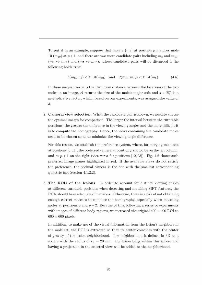
To put it in an example, suppose that mole 8 (m8) at position p matches mole
10 (m10) at p+ 1, and there are two more candidate pairs including m8 and m10:
(m8 ↔ m12) and (m7 ↔ m10). These candidate pairs will be discarded if the
following holds true:
d(m8,m7) < k ·A(m10) and d(m10,m12) < k ·A(m8). (4.5)
In these inequalities, d is the Euclidean distance between the locations of the two
moles in an image, A returns the size of the mole’s major axis and k ∈ R+1 is a
multiplicative factor, which, based on our experiments, was assigned the value of
3.
2. Camera/view selection. When the candidate pair is known, we need to choose
the optimal images for comparison. The larger the interval between the turntable
positions, the greater the difference in the viewing angles and the more difficult it
is to compute the homography. Hence, the views containing the candidate moles
need to be chosen so as to minimize the viewing angle difference.
For this reason, we establish the preference system, where, for merging mole sets
at positions [0, 11], the preferred camera at position p should be on the left column,
and at p + 1 on the right (vice-versa for positions [12, 23]). Fig. 4.6 shows such
preferred image planes highlighted in red. If the available views do not satisfy
the preference, the optimal camera is the one with the smallest corresponding
η-metric (see Section 4.1.2.2).
3. The ROIs of the lesions. In order to account for distinct viewing angles
at different turntable positions when detecting and matching SIFT features, the
ROIs should have adequate dimensions. Otherwise, there is a risk of not obtaining
enough correct matches to compute the homography, especially when matching
moles at positions p and p+ 2. Because of this, following a series of experiments
with images of different body regions, we increased the original 400× 400 ROI to
600× 600 pixels.
In addition, to make use of the visual information from the lesion’s neighbors in
the mole set, the ROI is extracted so that its center coincides with the center
of gravity of the lesion neighborhood. The neighborhood is defined in 3D as a
sphere with the radius of rn = 20 mm: any lesion lying within this sphere and
having a projection in the selected view will be added to the neighborhood.
85
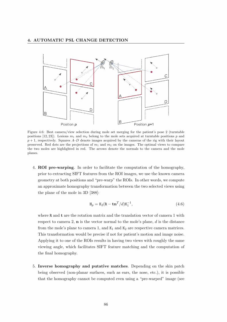
4. AUTOMATIC PSL CHANGE DETECTION
Figure 4.6: Best camera/view selection during mole set merging for the patient’s pose 2 (turntablepositions [12, 23]). Lesions m1 and m2 belong to the mole sets acquired at turntable positions p andp + 1, respectively. Squares A–D denote images acquired by the cameras of the rig with their layoutpreserved. Red dots are the projections of m1 and m2 on the images. The optimal views to comparethe two moles are highlighted in red. The arrows denote the normals to the camera and the moleplanes.
4. ROI pre-warping. In order to facilitate the computation of the homography,
prior to extracting SIFT features from the ROI images, we use the known camera
geometry at both positions and “pre-warp” the ROIs. In other words, we compute
an approximate homography transformation between the two selected views using
the plane of the mole in 3D [388]:
Hp = K2(R− tnT /d)K−11 , (4.6)
where R and t are the rotation matrix and the translation vector of camera 1 with
respect to camera 2, n is the vector normal to the mole’s plane, d is the distance
from the mole’s plane to camera 1, and K1 and K2 are respective camera matrices.
This transformation would be precise if not for patient’s motion and image noise.
Applying it to one of the ROIs results in having two views with roughly the same
viewing angle, which facilitates SIFT feature matching and the computation of
the final homography.
5. Inverse homography and putative matches. Depending on the skin patch
being observed (non-planar surfaces, such as ears, the nose, etc.), it is possible
that the homography cannot be computed even using a “pre-warped” image (see
86
Fig. 5.10 for an example). To deal with such cases, we make use of the inverse ho-
mographies. That is to say, given the left and right ROIs from different turntable
positions, we first find two “pre-homographies” to warp the left ROI onto the
right image, and vice versa. After that, we try to compute the homography
transformations for the two pairs of ROIs using SIFT features.
When a valid homography cannot be obtained for one of the pairs, it is probable
that the second pair will give a correct transformation. If this is not the case
(this may happen for the aforementioned areas when merging nonconsecutive
mole sets), the match is considered to be a putative match:
� The moles may represent the same or different real PSLs, but because of the
viewing angles neither statement can be confirmed.
When the merging procedure of the two mole sets has finished, some of the result-
ing putative matches can be pruned by simply checking if one of the candidate
moles was matched to any other mole. In a further stage of the mole match prop-
agation (see the next subsection), all putative matches are completely filtered.
6. Match condition. When the homographies between the two selected views have
been computed and the ROIs warped, it must be established whether the two vir-
tual moles represent the same real PSL. In most cases (especially for consecutive
mole sets) the matching ellipses will have their centers within each other’s bound-
aries. But due to the difference in the viewing angles and the skin patch topology,
it is possible that while not satisfying the “centers-in-the-boundaries” condition,
the two ellipses still represent the same real lesion. A straightforward workaround
for such cases would be to increase the allowed distance between the centers of
the ellipses. However, an opposite scenario is also possible—two virtual moles
representing different lesions can be located very close to each other (Fig. 4.7d),
making such thresholding inefficient. Thus, an alternative and more elaborate
condition is needed.
To ensure that all the scenarios shown in Fig. 4.7 are correctly resolved, an alter-
native condition should provide a trade-off between the relative dimensions of the
ellipses and the distance between their centers. Effectively, the two ellipses should
be considered matching if (1) the distance between their centers is comparable
with their minor axes and (2) their orientations are aligned.
The first requirement can be satisfied using the line connecting the centers of both
ellipses and the points where this line intersects them. The distance along this
87
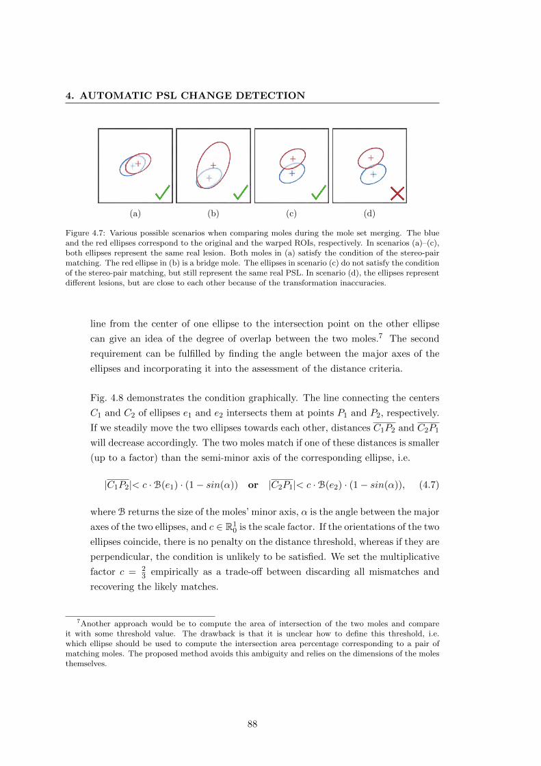
4. AUTOMATIC PSL CHANGE DETECTION
(a) (b) (c) (d)
Figure 4.7: Various possible scenarios when comparing moles during the mole set merging. The blueand the red ellipses correspond to the original and the warped ROIs, respectively. In scenarios (a)–(c),both ellipses represent the same real lesion. Both moles in (a) satisfy the condition of the stereo-pairmatching. The red ellipse in (b) is a bridge mole. The ellipses in scenario (c) do not satisfy the conditionof the stereo-pair matching, but still represent the same real PSL. In scenario (d), the ellipses representdifferent lesions, but are close to each other because of the transformation inaccuracies.
line from the center of one ellipse to the intersection point on the other ellipse
can give an idea of the degree of overlap between the two moles.7 The second
requirement can be fulfilled by finding the angle between the major axes of the
ellipses and incorporating it into the assessment of the distance criteria.
Fig. 4.8 demonstrates the condition graphically. The line connecting the centers
C1 and C2 of ellipses e1 and e2 intersects them at points P1 and P2, respectively.
If we steadily move the two ellipses towards each other, distances C1P2 and C2P1
will decrease accordingly. The two moles match if one of these distances is smaller
(up to a factor) than the semi-minor axis of the corresponding ellipse, i.e.
|C1P2|< c ·B(e1) · (1− sin(α)) or |C2P1|< c ·B(e2) · (1− sin(α)), (4.7)
where B returns the size of the moles’ minor axis, α is the angle between the major
axes of the two ellipses, and c ∈ R10 is the scale factor. If the orientations of the two
ellipses coincide, there is no penalty on the distance threshold, whereas if they are
perpendicular, the condition is unlikely to be satisfied. We set the multiplicative
factor c = 23 empirically as a trade-off between discarding all mismatches and
recovering the likely matches.
7Another approach would be to compute the area of intersection of the two moles and compareit with some threshold value. The drawback is that it is unclear how to define this threshold, i.e.which ellipse should be used to compute the intersection area percentage corresponding to a pair ofmatching moles. The proposed method avoids this ambiguity and relies on the dimensions of the molesthemselves.
88

Figure 4.8: The lesion matching condition during the mole set merging procedure. C1 and C2 are the
centers of ellipses e1 and e2, respectively. Line←−→C1C2 intersects e1 at point P1 and e2 at P2. The two
moles match if Eq. 4.7 is satisfied.
4.1.4.2 Mole match propagation
Once the mole sets have been merged at all successive turntable positions (p± 1,p± 2),
we need to run a recursive procedure to associate mole matches from nonsuccessive
positions (p ± x, where x ∈ Z>2). That is to say, two moles from mole sets A and B
can match another mole from set C, but not match each other (indirect match). The
objective of the association procedure is to make every mole match its counterparts
from other sets directly examining all indirect matches recursively. In this way, for
each mole of every set, there will be a group of lesions it matches in the rest of the sets.
The procedure is very similar to that described in Section 4.1.3, although the ex-
ceptions have to be resolved in a different manner. The main exception scenario also
involves bridge moles, whose simplest case is shown in Fig. 4.9a. Two moles from set
A as well as the mole in set C match the bridge mole in set B. As the result of the
recursive match propagation procedure, all the moles in the three sets will be grouped
to represent one real lesion.
Fortunately, it is easy to detect such exceptions, because in a group of virtual moles
representing a real lesion, there should not be more than one lesion per set.8 If this
condition is not satisfied, it indicates the presence of at least one bridge mole. However,
determining which one(s) of the moles is/are the bridge(s) is not as straightforward.
Ideally, it will be the lesion(s) directly matching two or more moles from the same mole
set. But not all bridges in a group can be discovered in this way, as there may be
several consecutive bridge moles, some of which are matched only to a single mole in
8In fact, it can happen that a bridge mole connects only single lesions in other mole sets. In thiscase, it is not possible to detect the exception, but the inconsistencies in the mole representation willnot be present either.
89
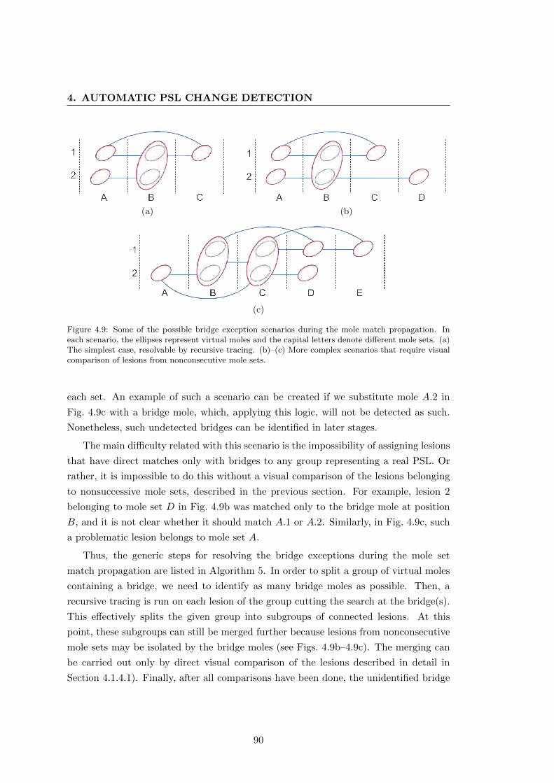
4. AUTOMATIC PSL CHANGE DETECTION
(a) (b)
(c)
Figure 4.9: Some of the possible bridge exception scenarios during the mole match propagation. Ineach scenario, the ellipses represent virtual moles and the capital letters denote different mole sets. (a)The simplest case, resolvable by recursive tracing. (b)–(c) More complex scenarios that require visualcomparison of lesions from nonconsecutive mole sets.
each set. An example of such a scenario can be created if we substitute mole A.2 in
Fig. 4.9c with a bridge mole, which, applying this logic, will not be detected as such.
Nonetheless, such undetected bridges can be identified in later stages.
The main difficulty related with this scenario is the impossibility of assigning lesions
that have direct matches only with bridges to any group representing a real PSL. Or
rather, it is impossible to do this without a visual comparison of the lesions belonging
to nonsuccessive mole sets, described in the previous section. For example, lesion 2
belonging to mole set D in Fig. 4.9b was matched only to the bridge mole at position
B, and it is not clear whether it should match A.1 or A.2. Similarly, in Fig. 4.9c, such
a problematic lesion belongs to mole set A.
Thus, the generic steps for resolving the bridge exceptions during the mole set
match propagation are listed in Algorithm 5. In order to split a group of virtual moles
containing a bridge, we need to identify as many bridge moles as possible. Then, a
recursive tracing is run on each lesion of the group cutting the search at the bridge(s).
This effectively splits the given group into subgroups of connected lesions. At this
point, these subgroups can still be merged further because lesions from nonconsecutive
mole sets may be isolated by the bridge moles (see Figs. 4.9b–4.9c). The merging can
be carried out only by direct visual comparison of the lesions described in detail in
Section 4.1.4.1). Finally, after all comparisons have been done, the unidentified bridge
90

Algorithm 5: Resolving a bridge exception during mole match propagation
Data: A group of virtual moles with bridge moles, gResult: A set of groups representing real lesions, G, the result of splitting g
1 /* Detect identifyable bridge lesions */
2 b← identifyBridgeMoles(g);3 /* Trace the direct matches of every mole in the group, trimming the
search at the bridges. Concatenate the obtained subgroups into a set.
*/
4 for all m in g do5 gTemp← traceMatches(m, b);6 G← concatenate(G, gTemp);
7 end8 /* Search for indirect matches: compare the groups in G visually and
merge the ones matching */
9 mm← compareSubgroups(G);10 G← mergeSubgroups(G,mm);11 /* Detect any unidentified bridge moles by checking for the repeating
moles across the subgroups */
12 b← identifyBridgeMoles(G)
moles can be detected by simply checking the subgroups for common lesions.
Once the matches have been propagated across all the turntable positions, the
mole map is ready. In fact, the map has the same structure as a mole set, with
the 3D locations and the local normals of the PSLs computed as the average of the
corresponding values in the matching mole sets. Similarly, each virtual mole will have
a number of corresponding 2D images from different viewpoints with a given η-metric
and px/mm resolution, which will be employed in the change detection procedure.
4.2 Inter-exploration operations
Two explorations of the patient’s skin surface performed several months apart can be
used for automatic detection of changes that individual lesions undergo over time (see
the general schema in Fig. 4.10). To do this, we only need to establish the correspon-
dences between the lesions of the two mole maps, i.e. given a PSL in one map, we have
to find which lesion it corresponds to on the other map. Once it has been done, the
change detection using the image patches around the moles is straightforward.
91
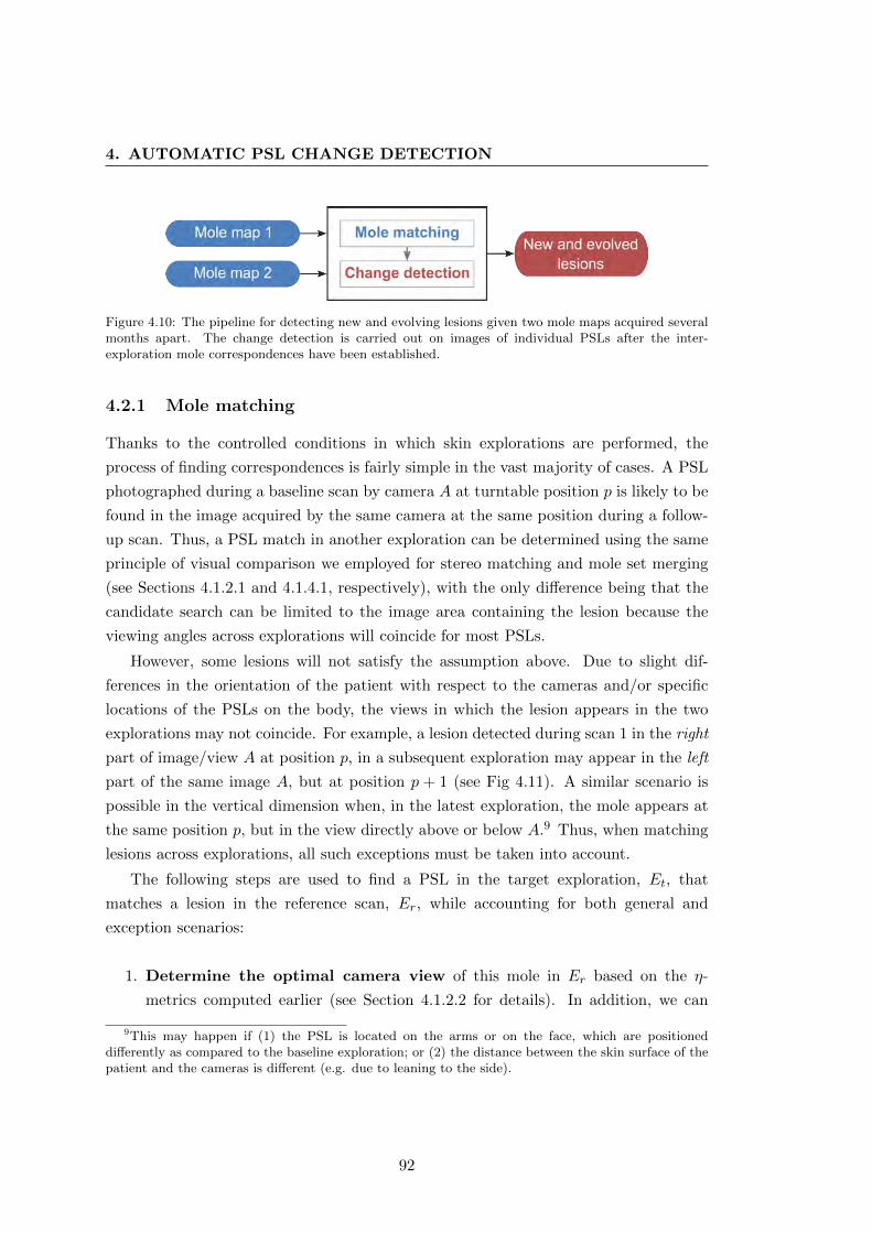
4. AUTOMATIC PSL CHANGE DETECTION
Figure 4.10: The pipeline for detecting new and evolving lesions given two mole maps acquired severalmonths apart. The change detection is carried out on images of individual PSLs after the inter-exploration mole correspondences have been established.
4.2.1 Mole matching
Thanks to the controlled conditions in which skin explorations are performed, the
process of finding correspondences is fairly simple in the vast majority of cases. A PSL
photographed during a baseline scan by camera A at turntable position p is likely to be
found in the image acquired by the same camera at the same position during a follow-
up scan. Thus, a PSL match in another exploration can be determined using the same
principle of visual comparison we employed for stereo matching and mole set merging
(see Sections 4.1.2.1 and 4.1.4.1, respectively), with the only difference being that the
candidate search can be limited to the image area containing the lesion because the
viewing angles across explorations will coincide for most PSLs.
However, some lesions will not satisfy the assumption above. Due to slight dif-
ferences in the orientation of the patient with respect to the cameras and/or specific
locations of the PSLs on the body, the views in which the lesion appears in the two
explorations may not coincide. For example, a lesion detected during scan 1 in the right
part of image/view A at position p, in a subsequent exploration may appear in the left
part of the same image A, but at position p + 1 (see Fig 4.11). A similar scenario is
possible in the vertical dimension when, in the latest exploration, the mole appears at
the same position p, but in the view directly above or below A.9 Thus, when matching
lesions across explorations, all such exceptions must be taken into account.
The following steps are used to find a PSL in the target exploration, Et, that
matches a lesion in the reference scan, Er, while accounting for both general and
exception scenarios:
1. Determine the optimal camera view of this mole in Er based on the η-
metrics computed earlier (see Section 4.1.2.2 for details). In addition, we can
9This may happen if (1) the PSL is located on the arms or on the face, which are positioneddifferently as compared to the baseline exploration; or (2) the distance between the skin surface of thepatient and the cameras is different (e.g. due to leaning to the side).
92
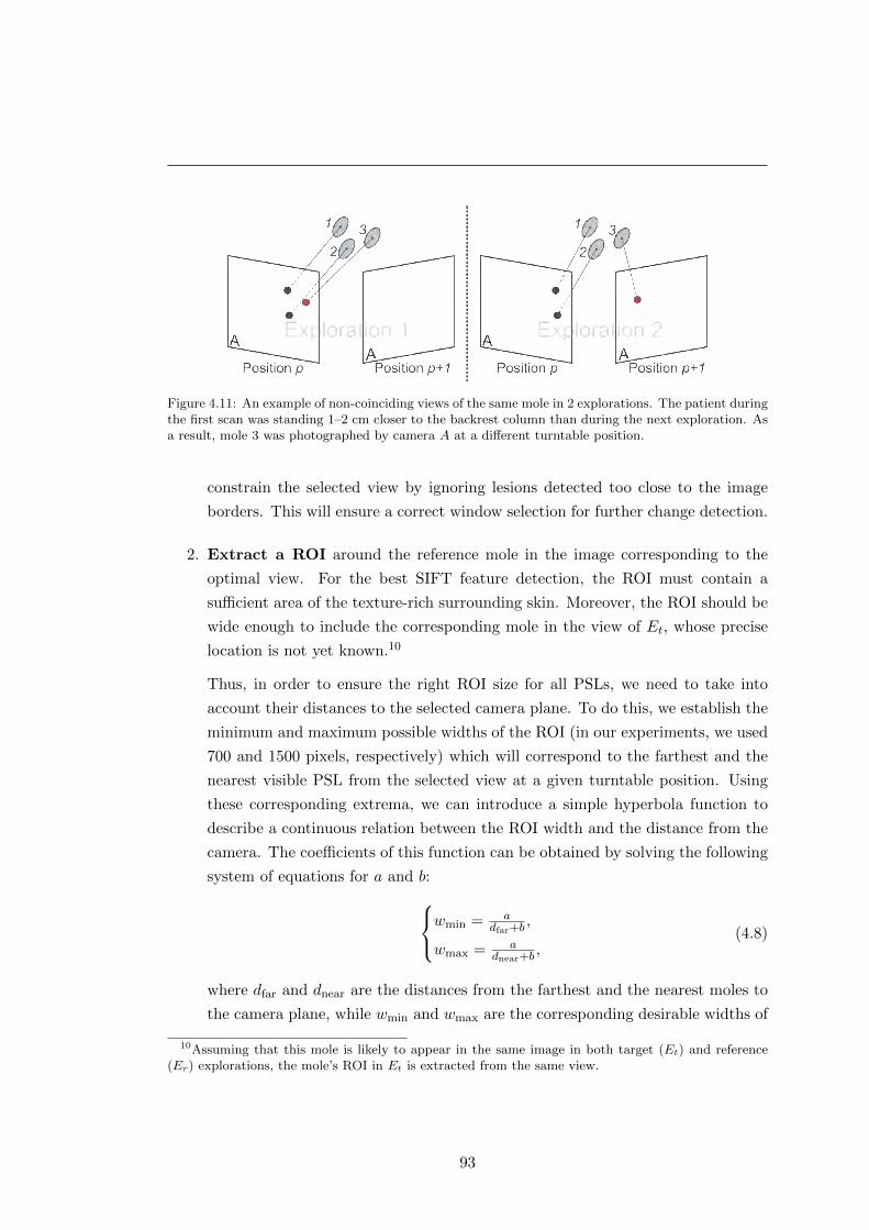
Figure 4.11: An example of non-coinciding views of the same mole in 2 explorations. The patient duringthe first scan was standing 1–2 cm closer to the backrest column than during the next exploration. Asa result, mole 3 was photographed by camera A at a different turntable position.
constrain the selected view by ignoring lesions detected too close to the image
borders. This will ensure a correct window selection for further change detection.
2. Extract a ROI around the reference mole in the image corresponding to the
optimal view. For the best SIFT feature detection, the ROI must contain a
sufficient area of the texture-rich surrounding skin. Moreover, the ROI should be
wide enough to include the corresponding mole in the view of Et, whose precise
location is not yet known.10
Thus, in order to ensure the right ROI size for all PSLs, we need to take into
account their distances to the selected camera plane. To do this, we establish the
minimum and maximum possible widths of the ROI (in our experiments, we used
700 and 1500 pixels, respectively) which will correspond to the farthest and the
nearest visible PSL from the selected view at a given turntable position. Using
these corresponding extrema, we can introduce a simple hyperbola function to
describe a continuous relation between the ROI width and the distance from the
camera. The coefficients of this function can be obtained by solving the following
system of equations for a and b:wmin = adfar+b
,
wmax = adnear+b
,(4.8)
where dfar and dnear are the distances from the farthest and the nearest moles to
the camera plane, while wmin and wmax are the corresponding desirable widths of
10Assuming that this mole is likely to appear in the same image in both target (Et) and reference(Er) explorations, the mole’s ROI in Et is extracted from the same view.
93
4. AUTOMATIC PSL CHANGE DETECTION
the ROI.
3. Compute the homography between the two ROIs and check its validity using
the condition described in Section 4.1.2.1. We can set the threshold to a higher
value (TH = 2500) because the two ROIs are going to have almost the same
viewing angle.
However, an erroneously computed homography means that the contents of the
two ROIs will differ significantly. This can happen because of (1) an abrupt
movement by the patient during the image acquisition, (2) a slightly different
arm positioning when assuming the pose, or (3) if the skin patch of the reference
mole is altered in Et (foreign marks on the skin, clothing, body hair, etc.). If the
failure happened due to (1) or (3), it will not be possible to establish the lesion
correspondence. However, if the homography could not be computed because of
a slight shift in the patient’s pose, selecting a different view will help. Hence,
we can try the available views in order to compute a valid homography, and if
none of the views produces one, we can assume that it is impossible to find the
correspondence automatically. That said, a reference lesion will not be matched
to a PSL in Et only if the image acquisition protocol is not followed precisely.
4. After the homography has been computed successfully, adjust the target im-
age ROI. Depending on the contents of the ROIs, after applying the computed
transformation, the following scenarios are possible:
(a) The target mole ellipse in Et is within the ROI and a smaller mole window11
can be extracted.
(b) The target mole ellipse is outside or too close to one of the ROI borders, but
is within the image boundaries and the mole window can be extracted (see
Fig. 4.12a).
(c) The ellipse is outside or too close to one of the image borders (Figs. 4.12b–c)
and the mole window cannot be extracted.
In the first scenario, we can proceed directly to subsequent steps in the algorithm,
while in the last two, we need to select a different ROI in either the same or
adjacent view acquired in Et. Thus, in scenario (b), we will simply need to
center the ROI on the ellipse projection and extract it from the same image
11A mole window is a small ROI image big enough only to contain the entire PSL and is necessaryfor the change detection phase.
94
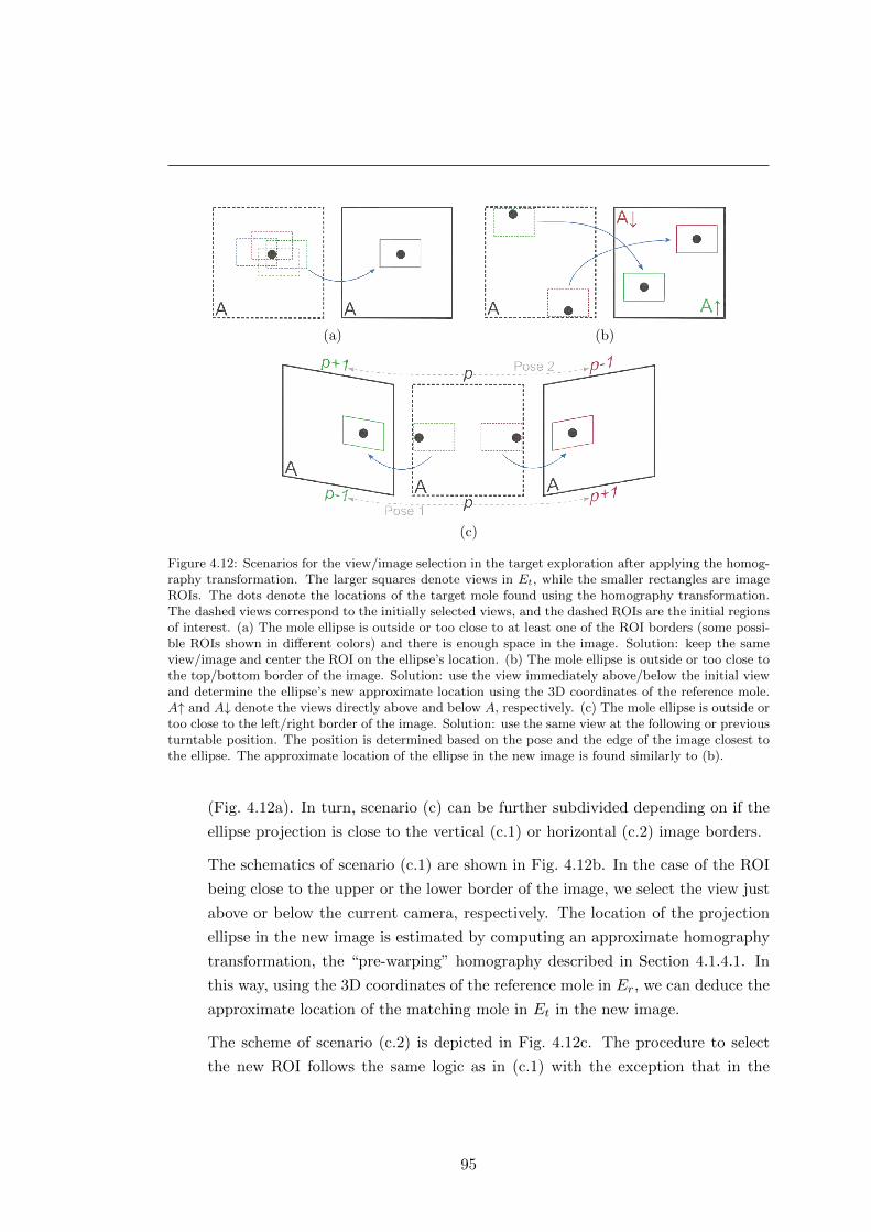
(a) (b)
(c)
Figure 4.12: Scenarios for the view/image selection in the target exploration after applying the homog-raphy transformation. The larger squares denote views in Et, while the smaller rectangles are imageROIs. The dots denote the locations of the target mole found using the homography transformation.The dashed views correspond to the initially selected views, and the dashed ROIs are the initial regionsof interest. (a) The mole ellipse is outside or too close to at least one of the ROI borders (some possi-ble ROIs shown in different colors) and there is enough space in the image. Solution: keep the sameview/image and center the ROI on the ellipse’s location. (b) The mole ellipse is outside or too close tothe top/bottom border of the image. Solution: use the view immediately above/below the initial viewand determine the ellipse’s new approximate location using the 3D coordinates of the reference mole.A↑ and A↓ denote the views directly above and below A, respectively. (c) The mole ellipse is outside ortoo close to the left/right border of the image. Solution: use the same view at the following or previousturntable position. The position is determined based on the pose and the edge of the image closest tothe ellipse. The approximate location of the ellipse in the new image is found similarly to (b).
(Fig. 4.12a). In turn, scenario (c) can be further subdivided depending on if the
ellipse projection is close to the vertical (c.1) or horizontal (c.2) image borders.
The schematics of scenario (c.1) are shown in Fig. 4.12b. In the case of the ROI
being close to the upper or the lower border of the image, we select the view just
above or below the current camera, respectively. The location of the projection
ellipse in the new image is estimated by computing an approximate homography
transformation, the “pre-warping” homography described in Section 4.1.4.1. In
this way, using the 3D coordinates of the reference mole in Er, we can deduce the
approximate location of the matching mole in Et in the new image.
The scheme of scenario (c.2) is depicted in Fig. 4.12c. The procedure to select
the new ROI follows the same logic as in (c.1) with the exception that in the
95
4. AUTOMATIC PSL CHANGE DETECTION
absence of horizontally adjacent views, we select the images acquired at other
turntable positions. Concretely, depending on the pose of the patient (direction
of the turntable rotation) and whether the lesion is closer to the left or the right
border of the image, we select either the next or the previous turntable position,
as shown in the figure.
After acquiring the new ROI in Et, we register the reference and the target ROIs
by once again computing the homography transformation using SIFT feature
matching.
5. Obtain the ellipse of the target mole. This ellipse is needed to extract
a target mole window of adequate size for the change detection as well as to
determine the index of the matching mole in the map of Et. If the ellipse was
detected in the Et mole mapping stage, it can be identified by means of a simple
distance threshold. However, it can either form part of the mole map or not
(the mole could not be matched with other lesions in the stereo pairs or at other
turntable positions).
If it is a new lesion, or if this PSL was not detected during the mapping proce-
dure, it must be segmented using MSER. For this purpose, we use the procedure
described in Section 4.1.1.
6. Extract mole windows from the reference and the target ROIs using the mole
ellipses. The side of the window is equal to
N = 2 · l ·max(A(mr),A(mt)), (4.9)
where mr and mt are the ellipses of the moles in Er and Et, respectively, function
A returns the size of the mole’s major axis and l is a scale coefficient (in our
experiments, we used l = 1.5). However, at this stage, the size of the window
around mt is multiplied by 1.5 for the subsequent stage of image alignment by
translation.
7. Register mole windows by means of the weighted normalized cross-
correlation (NCC). This step is important for a more precise alignment of the
two mole windows. The NCC [398] is performed on the normalized blue channels
of the images, which provides the best skin-lesion contrast and, at the same time,
eliminates weak artifacts such as hair or skin pores. In addition, the area of
the lesion in the window containing mr is weighted, so that significantly more
96
emphasis is put on the relevant pixels.
8. Prepare the mole masks. The binary masks specifying the PSL area in the
mole windows can be obtained using the MSER segmentations computed earlier
(see Section 4.1.1). These segmentations need only to be fit into the windows at
the locations of the mole ellipses.
After all the steps of the algorithm have been performed, for each PSL there will
be a pair of aligned images acquired in the two explorations. These images can be used
for the assessment of changes the lesion has undergone before the follow-up screening.
4.2.2 Change detection
With the aligned mole images and masks extracted from the reference and the target
explorations, the detection of changes in a lesion is straightforward. It is important to
note that we do not intend to describe the changes precisely. Rather, the goal is to
be able to indicate to the physician that certain PSLs are undergoing changes and are
worth a closer examination. In addition, parameterizing the importance of the change
should give a way of controlling noise tolerance in the system’s output.
Algorithm 6 shows the basic steps needed to acquire the change mask of a lesion
from two consecutive scans. At first, the images of the lesion are converted to the
HSV representation, since it allows a more intuitive description of the changes in the
appearance, clearly separating color and saturation. Then we compute a difference
image using each channel individually (hue, saturation, value). This image shows how
each pixel in one image is different from its corresponding pixel in the other image.
From the difference image we generate the gray-level change map by finding the
maximum value of each pixel across all channels and applying a median filter to remove
spurious noise. Now, this map can be binarized using the threshold provided, which, in
our experiments, was set to Tb = 0.1. This parameter allows controlling how sensitive
the system is going to be to the changes detected.
Finally, we combine the lesion masks from both images into one unified mask which
defines the area where change is to be sought. In order to keep only the changes
that occurred within the PSL and not in the surrounding skin, the binary change map
obtained is merged with this unified lesion mask. Using the ratio of the total change area
to the area of the mask, we can parameterize the importance of the lesion’s evolution.
For example, if we set this parameter to Tc = 0.15, the lesions with 15% of their area
altered will be considered as undergoing important changes.
97
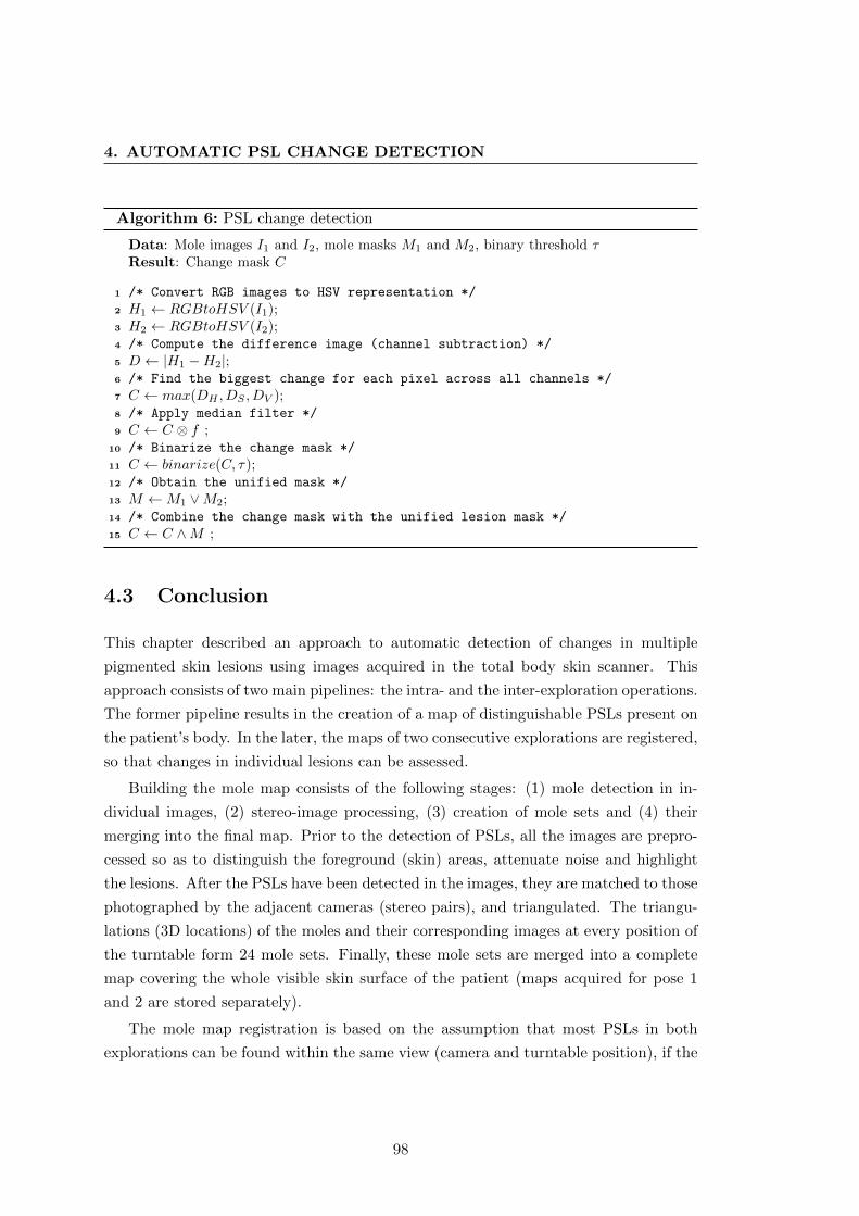
4. AUTOMATIC PSL CHANGE DETECTION
Algorithm 6: PSL change detection
Data: Mole images I1 and I2, mole masks M1 and M2, binary threshold τResult: Change mask C
1 /* Convert RGB images to HSV representation */
2 H1 ← RGBtoHSV (I1);3 H2 ← RGBtoHSV (I2);4 /* Compute the difference image (channel subtraction) */
5 D ← |H1 −H2|;6 /* Find the biggest change for each pixel across all channels */
7 C ← max(DH , DS , DV );8 /* Apply median filter */
9 C ← C ⊗ f ;10 /* Binarize the change mask */
11 C ← binarize(C, τ);12 /* Obtain the unified mask */
13 M ←M1 ∨M2;14 /* Combine the change mask with the unified lesion mask */
15 C ← C ∧M ;
4.3 Conclusion
This chapter described an approach to automatic detection of changes in multiple
pigmented skin lesions using images acquired in the total body skin scanner. This
approach consists of two main pipelines: the intra- and the inter-exploration operations.
The former pipeline results in the creation of a map of distinguishable PSLs present on
the patient’s body. In the later, the maps of two consecutive explorations are registered,
so that changes in individual lesions can be assessed.
Building the mole map consists of the following stages: (1) mole detection in in-
dividual images, (2) stereo-image processing, (3) creation of mole sets and (4) their
merging into the final map. Prior to the detection of PSLs, all the images are prepro-
cessed so as to distinguish the foreground (skin) areas, attenuate noise and highlight
the lesions. After the PSLs have been detected in the images, they are matched to those
photographed by the adjacent cameras (stereo pairs), and triangulated. The triangu-
lations (3D locations) of the moles and their corresponding images at every position of
the turntable form 24 mole sets. Finally, these mole sets are merged into a complete
map covering the whole visible skin surface of the patient (maps acquired for pose 1
and 2 are stored separately).
The mole map registration is based on the assumption that most PSLs in both
explorations can be found within the same view (camera and turntable position), if the
98
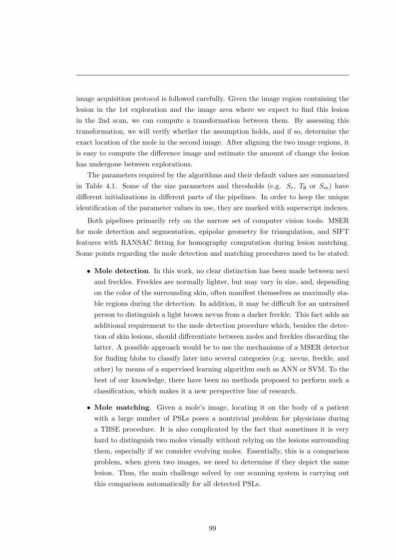
image acquisition protocol is followed carefully. Given the image region containing the
lesion in the 1st exploration and the image area where we expect to find this lesion
in the 2nd scan, we can compute a transformation between them. By assessing this
transformation, we will verify whether the assumption holds, and if so, determine the
exact location of the mole in the second image. After aligning the two image regions, it
is easy to compute the difference image and estimate the amount of change the lesion
has undergone between explorations.
The parameters required by the algorithms and their default values are summarized
in Table 4.1. Some of the size parameters and thresholds (e.g. Sr, TH or Sm) have
different initializations in different parts of the pipelines. In order to keep the unique
identification of the parameter values in use, they are marked with superscript indexes.
Both pipelines primarily rely on the narrow set of computer vision tools: MSER
for mole detection and segmentation, epipolar geometry for triangulation, and SIFT
features with RANSAC fitting for homography computation during lesion matching.
Some points regarding the mole detection and matching procedures need to be stated:
� Mole detection. In this work, no clear distinction has been made between nevi
and freckles. Freckles are normally lighter, but may vary in size, and, depending
on the color of the surrounding skin, often manifest themselves as maximally sta-
ble regions during the detection. In addition, it may be difficult for an untrained
person to distinguish a light brown nevus from a darker freckle. This fact adds an
additional requirement to the mole detection procedure which, besides the detec-
tion of skin lesions, should differentiate between moles and freckles discarding the
latter. A possible approach would be to use the mechanisms of a MSER detector
for finding blobs to classify later into several categories (e.g. nevus, freckle, and
other) by means of a supervised learning algorithm such as ANN or SVM. To the
best of our knowledge, there have been no methods proposed to perform such a
classification, which makes it a new perspective line of research.
� Mole matching. Given a mole’s image, locating it on the body of a patient
with a large number of PSLs poses a nontrivial problem for physicians during
a TBSE procedure. It is also complicated by the fact that sometimes it is very
hard to distinguish two moles visually without relying on the lesions surrounding
them, especially if we consider evolving moles. Essentially, this is a comparison
problem, when given two images, we need to determine if they depict the same
lesion. Thus, the main challenge solved by our scanning system is carrying out
this comparison automatically for all detected PSLs.
99
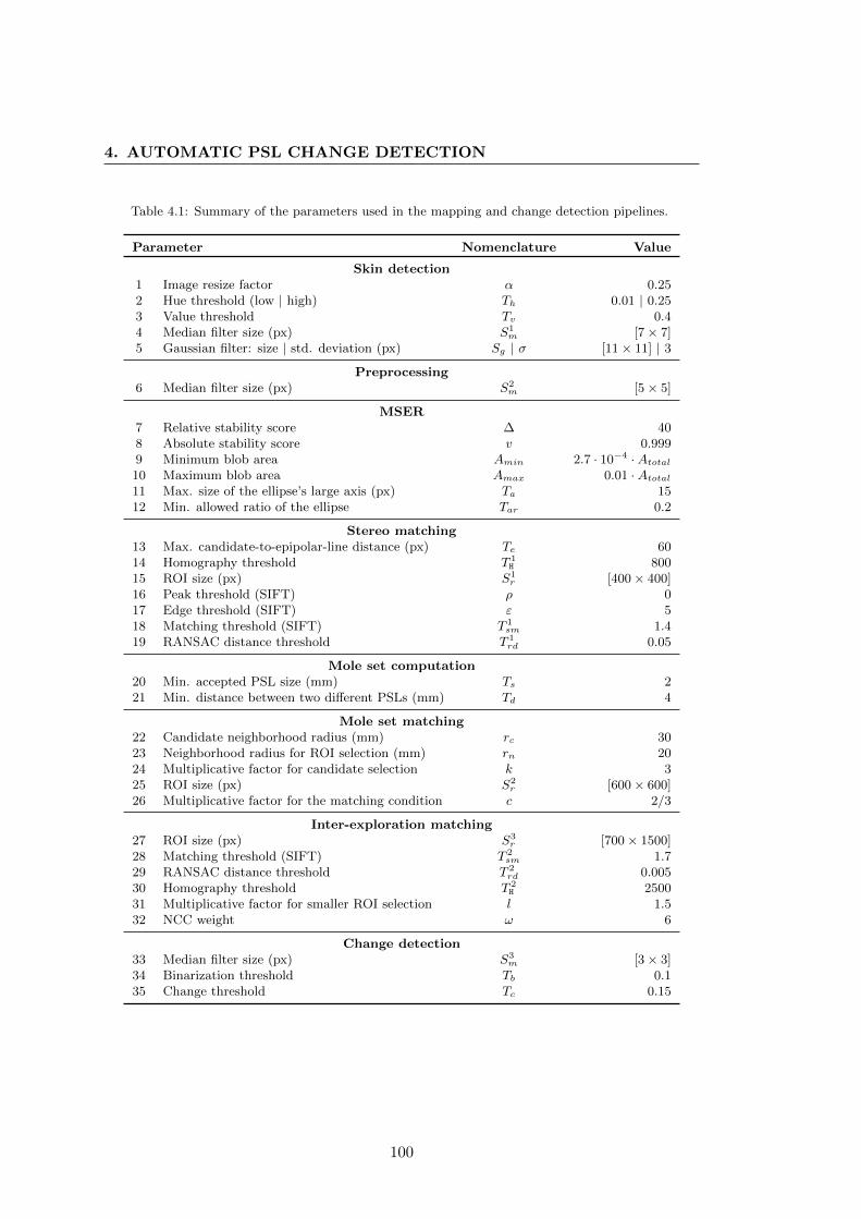
4. AUTOMATIC PSL CHANGE DETECTION
Table 4.1: Summary of the parameters used in the mapping and change detection pipelines.
Parameter Nomenclature Value
Skin detection1 Image resize factor α 0.252 Hue threshold (low | high) Th 0.01 | 0.253 Value threshold Tv 0.44 Median filter size (px) S1
m [7× 7]5 Gaussian filter: size | std. deviation (px) Sg | σ [11× 11] | 3
Preprocessing6 Median filter size (px) S2
m [5× 5]
MSER7 Relative stability score ∆ 408 Absolute stability score v 0.9999 Minimum blob area Amin 2.7 · 10−4 ·Atotal10 Maximum blob area Amax 0.01 ·Atotal11 Max. size of the ellipse’s large axis (px) Ta 1512 Min. allowed ratio of the ellipse Tar 0.2
Stereo matching13 Max. candidate-to-epipolar-line distance (px) Te 6014 Homography threshold T 1
H 80015 ROI size (px) S1
r [400× 400]16 Peak threshold (SIFT) ρ 017 Edge threshold (SIFT) ε 518 Matching threshold (SIFT) T 1
sm 1.419 RANSAC distance threshold T 1
rd 0.05
Mole set computation20 Min. accepted PSL size (mm) Ts 221 Min. distance between two different PSLs (mm) Td 4
Mole set matching22 Candidate neighborhood radius (mm) rc 3023 Neighborhood radius for ROI selection (mm) rn 2024 Multiplicative factor for candidate selection k 325 ROI size (px) S2
r [600× 600]26 Multiplicative factor for the matching condition c 2/3
Inter-exploration matching27 ROI size (px) S3
r [700× 1500]28 Matching threshold (SIFT) T 2
sm 1.729 RANSAC distance threshold T 2
rd 0.00530 Homography threshold T 2
H 250031 Multiplicative factor for smaller ROI selection l 1.532 NCC weight ω 6
Change detection33 Median filter size (px) S3
m [3× 3]34 Binarization threshold Tb 0.135 Change threshold Tc 0.15
100

In the same way as physicians constrain their search by knowing the region of the
body depicted in an image, our system uses the known geometry of the cameras.
However, our approach to determine the precise location of a mole is different.
Unlike physicians, who normally refine their search using the moles’ dermoscopic
structures, the proposed system relies strongly on the visual information of the
skin surrounding the mole. One of the drawbacks of such an approach is that it
can be sensitive to the viewing angle of the cameras.
For instance, the appearance of a mole located on the medial border of the shoul-
der blade can vary in two images to an extent that it is impossible to find corre-
sponding SIFT features. This may happen when comparing mole images acquired
at the pth and (p + 2)th turntable positions. In such cases, it is unclear whether
two images depict the same lesion, so the result is considered to be a putative
match until it can be resolved by the match association procedure.
A putative match cannot be resolved only when one of the moles does not have
any matches in other mole sets. However, we discard such lesions, because, as
experiments have shown, these are less stable and/or undersized moles/freckles
which are not yet of interest for future change detection. But if, with time, these
lesions enlarge or grow darker, they will be automatically detected during the
exploration and compared with the baseline.
The experimental results of applying the proposed algorithms to real data are dis-
cussed in the next chapter.
101

4. AUTOMATIC PSL CHANGE DETECTION
102

...we must reinforce argument with results.
“The Booker T. Washington Papers: 1903–4” [399]
Chapter 5
Results and discussion
This chapter presents experimental results of the algorithms for the automatic PSL
change detection in images acquired using the total body skin scanner described in
Chapter 3. All input parameters for the algorithms were set empirically during the
experiments. The results reported herein contain all necessary references to the de-
scription of the algorithms.
5.1 Intra-exploration operations
In each of the following subsections, we analyze and discuss the performance of indi-
vidual stages of the mole mapping pipeline (intra-exploration operations).
5.1.1 Skin detection
Prior to the image processing and detection of PSLs on the patient’s body, we generate
a “skin mask”: a binary image that defines the foreground area where the lesions are to
be detected. This mask is essential for a correct estimation of the skin’s intensity ranges
during the preprocessing stage. It is also useful for discarding MSER blobs detected
on background elements such as the backrest column. This algorithm was described in
Section 4.1.1.1, and the results of its application to the scanner’s image data are shown
in Fig. 5.1.
As illustrated in the figure, the approach, although simple, allows for correct de-
tection of skin of different types without producing many artifacts. Figs. 5.1a and b
demonstrate a successful detection even in the presence of a tanned skin and clothing.
A slight inconsistency in the masks can be seen in shaded underlit areas, for example,
in Figs. 5.1c or 5.1e. In the former, it is the area of the chin, while in the latter, it is the
103
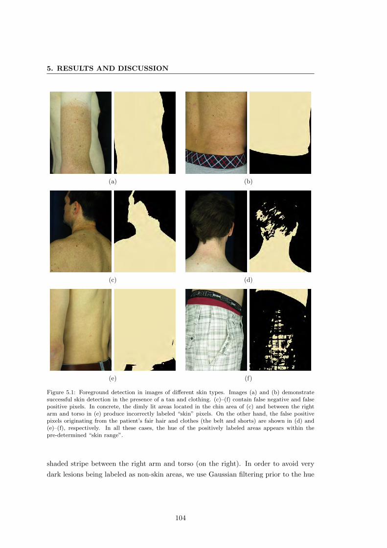
5. RESULTS AND DISCUSSION
(a) (b)
(c) (d)
(e) (f)
Figure 5.1: Foreground detection in images of different skin types. Images (a) and (b) demonstratesuccessful skin detection in the presence of a tan and clothing. (c)–(f) contain false negative and falsepositive pixels. In concrete, the dimly lit areas located in the chin area of (c) and between the rightarm and torso in (e) produce incorrectly labeled “skin” pixels. On the other hand, the false positivepixels originating from the patient’s fair hair and clothes (the belt and shorts) are shown in (d) and(e)–(f), respectively. In all these cases, the hue of the positively labeled areas appears within thepre-determined “skin range”.
shaded stripe between the right arm and torso (on the right). In order to avoid very
dark lesions being labeled as non-skin areas, we use Gaussian filtering prior to the hue
104
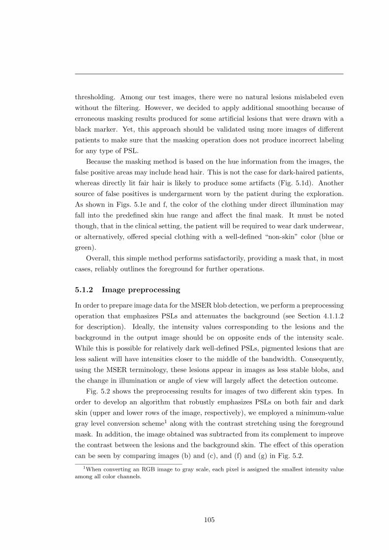
thresholding. Among our test images, there were no natural lesions mislabeled even
without the filtering. However, we decided to apply additional smoothing because of
erroneous masking results produced for some artificial lesions that were drawn with a
black marker. Yet, this approach should be validated using more images of different
patients to make sure that the masking operation does not produce incorrect labeling
for any type of PSL.
Because the masking method is based on the hue information from the images, the
false positive areas may include head hair. This is not the case for dark-haired patients,
whereas directly lit fair hair is likely to produce some artifacts (Fig. 5.1d). Another
source of false positives is undergarment worn by the patient during the exploration.
As shown in Figs. 5.1e and f, the color of the clothing under direct illumination may
fall into the predefined skin hue range and affect the final mask. It must be noted
though, that in the clinical setting, the patient will be required to wear dark underwear,
or alternatively, offered special clothing with a well-defined “non-skin” color (blue or
green).
Overall, this simple method performs satisfactorily, providing a mask that, in most
cases, reliably outlines the foreground for further operations.
5.1.2 Image preprocessing
In order to prepare image data for the MSER blob detection, we perform a preprocessing
operation that emphasizes PSLs and attenuates the background (see Section 4.1.1.2
for description). Ideally, the intensity values corresponding to the lesions and the
background in the output image should be on opposite ends of the intensity scale.
While this is possible for relatively dark well-defined PSLs, pigmented lesions that are
less salient will have intensities closer to the middle of the bandwidth. Consequently,
using the MSER terminology, these lesions appear in images as less stable blobs, and
the change in illumination or angle of view will largely affect the detection outcome.
Fig. 5.2 shows the preprocessing results for images of two different skin types. In
order to develop an algorithm that robustly emphasizes PSLs on both fair and dark
skin (upper and lower rows of the image, respectively), we employed a minimum-value
gray level conversion scheme1 along with the contrast stretching using the foreground
mask. In addition, the image obtained was subtracted from its complement to improve
the contrast between the lesions and the background skin. The effect of this operation
can be seen by comparing images (b) and (c), and (f) and (g) in Fig. 5.2.
1When converting an RGB image to gray scale, each pixel is assigned the smallest intensity valueamong all color channels.
105
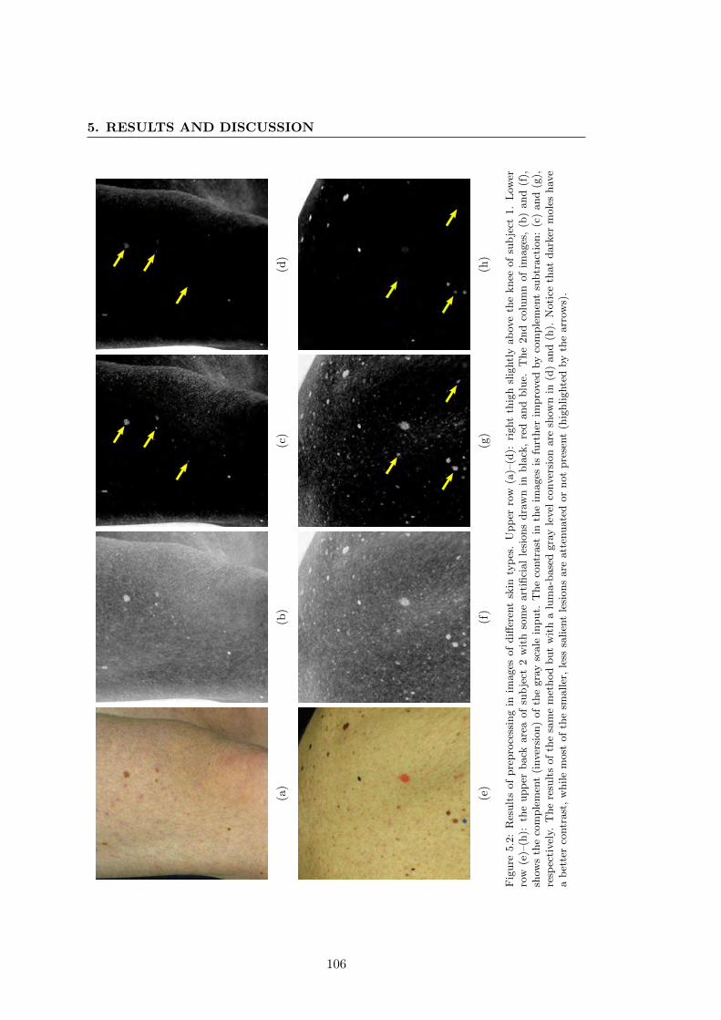
5. RESULTS AND DISCUSSION
(a)
(b)
(c)
(d)
(e)
(f)
(g)
(h)
Fig
ure
5.2
:R
esult
sof
pre
pro
cess
ing
inim
ages
of
diff
eren
tsk
inty
pes
.U
pp
erro
w(a
)–(d
):ri
ght
thig
hsl
ightl
yab
ove
the
knee
of
sub
ject
1.
Low
erro
w(e
)–(h
):th
eupp
erback
are
aof
sub
ject
2w
ith
som
eart
ifici
al
lesi
ons
dra
wn
inbla
ck,
red
and
blu
e.T
he
2nd
colu
mn
of
images
,(b
)and
(f),
show
sth
eco
mple
men
t(i
nver
sion)
of
the
gra
ysc
ale
input.
The
contr
ast
inth
eim
ages
isfu
rther
impro
ved
by
com
ple
men
tsu
btr
act
ion:
(c)
and
(g),
resp
ecti
vel
y.T
he
resu
lts
of
the
sam
em
ethod
but
wit
ha
lum
a-b
ase
dgra
yle
vel
conver
sion
are
show
nin
(d)
and
(h).
Noti
ceth
at
dark
erm
ole
shav
ea
bet
ter
contr
ast
,w
hile
most
of
the
smaller
,le
sssa
lien
tle
sions
are
att
enuate
dor
not
pre
sent
(hig
hlighte
dby
the
arr
ows)
.
106
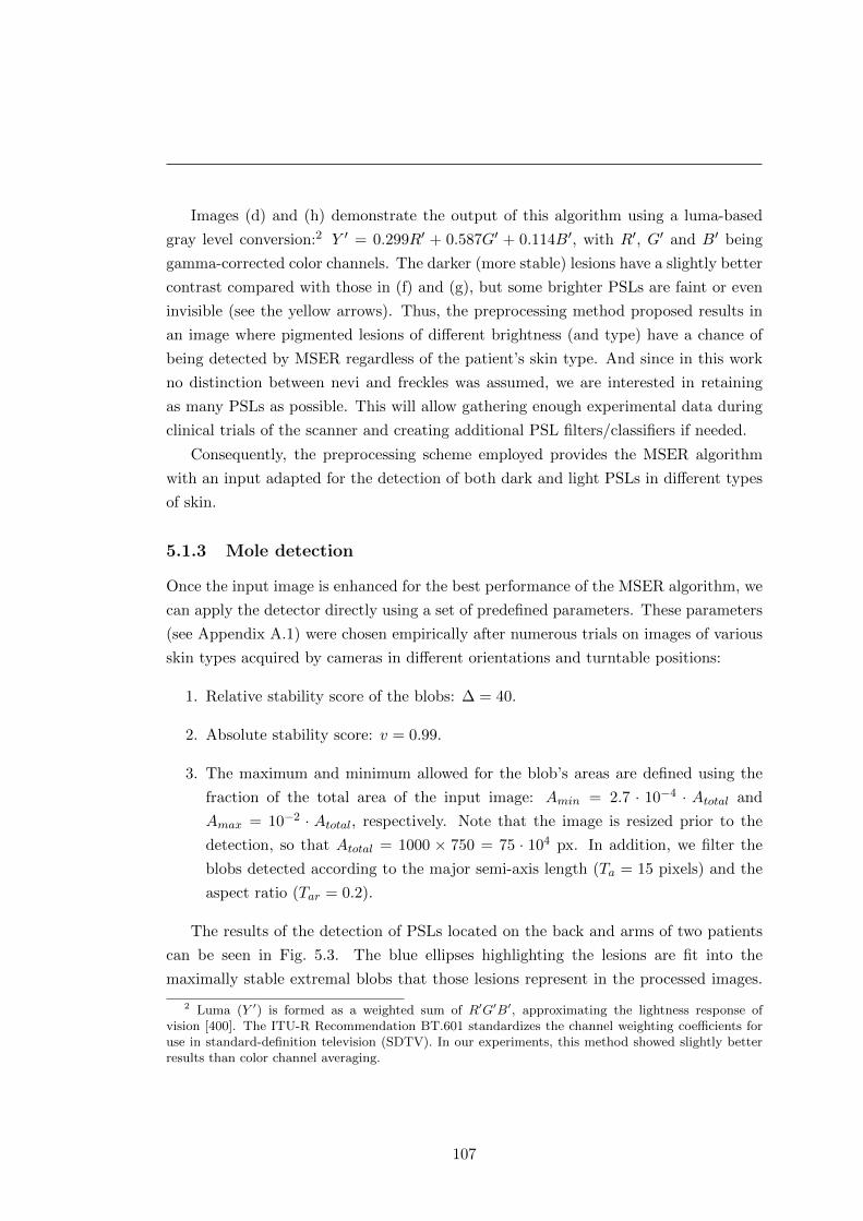
Images (d) and (h) demonstrate the output of this algorithm using a luma-based
gray level conversion:2 Y ′ = 0.299R′ + 0.587G′ + 0.114B′, with R′, G′ and B′ being
gamma-corrected color channels. The darker (more stable) lesions have a slightly better
contrast compared with those in (f) and (g), but some brighter PSLs are faint or even
invisible (see the yellow arrows). Thus, the preprocessing method proposed results in
an image where pigmented lesions of different brightness (and type) have a chance of
being detected by MSER regardless of the patient’s skin type. And since in this work
no distinction between nevi and freckles was assumed, we are interested in retaining
as many PSLs as possible. This will allow gathering enough experimental data during
clinical trials of the scanner and creating additional PSL filters/classifiers if needed.
Consequently, the preprocessing scheme employed provides the MSER algorithm
with an input adapted for the detection of both dark and light PSLs in different types
of skin.
5.1.3 Mole detection
Once the input image is enhanced for the best performance of the MSER algorithm, we
can apply the detector directly using a set of predefined parameters. These parameters
(see Appendix A.1) were chosen empirically after numerous trials on images of various
skin types acquired by cameras in different orientations and turntable positions:
1. Relative stability score of the blobs: ∆ = 40.
2. Absolute stability score: v = 0.99.
3. The maximum and minimum allowed for the blob’s areas are defined using the
fraction of the total area of the input image: Amin = 2.7 · 10−4 · Atotal and
Amax = 10−2 · Atotal, respectively. Note that the image is resized prior to the
detection, so that Atotal = 1000 × 750 = 75 · 104 px. In addition, we filter the
blobs detected according to the major semi-axis length (Ta = 15 pixels) and the
aspect ratio (Tar = 0.2).
The results of the detection of PSLs located on the back and arms of two patients
can be seen in Fig. 5.3. The blue ellipses highlighting the lesions are fit into the
maximally stable extremal blobs that those lesions represent in the processed images.
2 Luma (Y ′) is formed as a weighted sum of R′G′B′, approximating the lightness response ofvision [400]. The ITU-R Recommendation BT.601 standardizes the channel weighting coefficients foruse in standard-definition television (SDTV). In our experiments, this method showed slightly betterresults than color channel averaging.
107
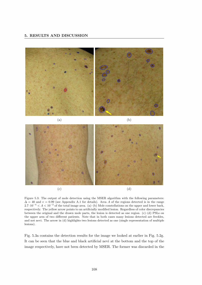
5. RESULTS AND DISCUSSION
(a) (b)
(c) (d)
Figure 5.3: The output of mole detection using the MSER algorithm with the following parameters:∆ = 40 and v = 0.99 (see Appendix A.1 for details). Area A of the regions detected is in the range2.7 ·10−4 < A < 10−2 of the total image area. (a)–(b) Mole constellations on the upper and lower back,respectively. The yellow arrow points to an artificially modified lesion. Regardless of color discrepanciesbetween the original and the drawn mole parts, the lesion is detected as one region. (c)–(d) PSLs onthe upper arm of two different patients. Note that in both cases many lesions detected are freckles,and not nevi. The arrow in (d) highlights two lesions detected as one (single representation of multiplelesions).
Fig. 5.3a contains the detection results for the image we looked at earlier in Fig. 5.2g.
It can be seen that the blue and black artificial nevi at the bottom and the top of the
image respectively, have not been detected by MSER. The former was discarded in the
108
skin masking stage because bright blue is outside the defined skin color range. The
latter mole is located in the dimly-lit area, so the contrast between the lesion and the
skin does not meet the limitations imposed by the MSER parameters. This could be
improved by using an illumination correction algorithm or an adaptive procedure for
local contrast enhancement. However, the drawback with these approaches would be an
unnecessary amplification of other skin details such as hairs, pores or spots. Besides,
the goal is not to detect all PSLs in one image, but rather concentrate on those in
the best lit central area of the image. This is because we want to have the best view
possible of each lesion (good lighting conditions, minimum body curvature, best angle
of view) in order to assess the changes correctly. At the same time, multiple cameras
and a sufficient number of turntable steps give a certain freedom to discarding less
suitable lesion images.
In Fig. 5.3b, all the PSLs have been detected correctly, including a mole with an
artificial change indicated by an arrow. The lesions detected in Figs. 5.3c and d are
mostly freckles. Because the arms appear closer to the cameras during the image
acquisition, the resolution in that area is better and it is easier for the algorithm to
distinguish even the smallest PSL. One future improvement of this system will include
a dynamic threshold definition for the minimum/maximum lesion size depending on
the turntable’s position at which the images were acquired.
An example of a single representation of two lesions, as discussed in Section 4.1.3.2,
can be appreciated in Fig. 5.3d. Despite the fact that one of the two PSLs is a light
freckle, in images acquired at different positions, or by a neighboring camera, they
can be detected as a single lesion, causing a special situation during mole set creation
or merging. These cases can be recognized and corrected by means of the heuristics
described in the previous chapter.
In conclusion, the MSER algorithm is a powerful tool for the detection and coarse
segmentation of multiple PSLs. Since its output is largely dependent on the intensity
information of the input image, we can modify it to direct the method towards the result
we want to obtain. Additionally, its output can be further improved by controlling the
size limitations of the lesions detected as well as by applying machine learning to identify
their types.
5.1.4 Mole matching in stereo pairs
In order to identify a skin lesion in a stereo pair, one must carry out a comparison of
the moles’ visual properties, such as size and shape. Human observers normally rely
109
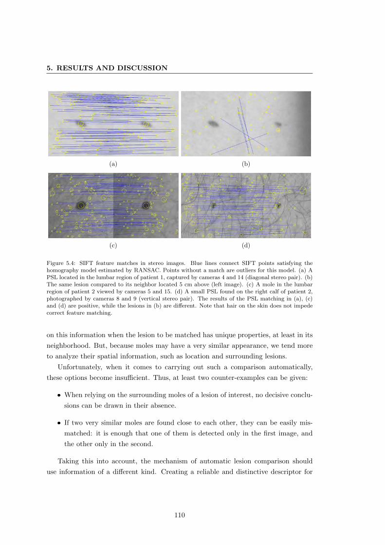
5. RESULTS AND DISCUSSION
(a) (b)
(c) (d)
Figure 5.4: SIFT feature matches in stereo images. Blue lines connect SIFT points satisfying thehomography model estimated by RANSAC. Points without a match are outliers for this model. (a) APSL located in the lumbar region of patient 1, captured by cameras 4 and 14 (diagonal stereo pair). (b)The same lesion compared to its neighbor located 5 cm above (left image). (c) A mole in the lumbarregion of patient 2 viewed by cameras 5 and 15. (d) A small PSL found on the right calf of patient 2,photographed by cameras 8 and 9 (vertical stereo pair). The results of the PSL matching in (a), (c)and (d) are positive, while the lesions in (b) are different. Note that hair on the skin does not impedecorrect feature matching.
on this information when the lesion to be matched has unique properties, at least in its
neighborhood. But, because moles may have a very similar appearance, we tend more
to analyze their spatial information, such as location and surrounding lesions.
Unfortunately, when it comes to carrying out such a comparison automatically,
these options become insufficient. Thus, at least two counter-examples can be given:
� When relying on the surrounding moles of a lesion of interest, no decisive conclu-
sions can be drawn in their absence.
� If two very similar moles are found close to each other, they can be easily mis-
matched: it is enough that one of them is detected only in the first image, and
the other only in the second.
Taking this into account, the mechanism of automatic lesion comparison should
use information of a different kind. Creating a reliable and distinctive descriptor for
110
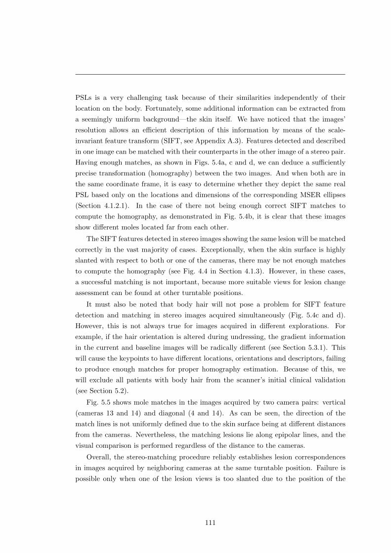
PSLs is a very challenging task because of their similarities independently of their
location on the body. Fortunately, some additional information can be extracted from
a seemingly uniform background—the skin itself. We have noticed that the images’
resolution allows an efficient description of this information by means of the scale-
invariant feature transform (SIFT, see Appendix A.3). Features detected and described
in one image can be matched with their counterparts in the other image of a stereo pair.
Having enough matches, as shown in Figs. 5.4a, c and d, we can deduce a sufficiently
precise transformation (homography) between the two images. And when both are in
the same coordinate frame, it is easy to determine whether they depict the same real
PSL based only on the locations and dimensions of the corresponding MSER ellipses
(Section 4.1.2.1). In the case of there not being enough correct SIFT matches to
compute the homography, as demonstrated in Fig. 5.4b, it is clear that these images
show different moles located far from each other.
The SIFT features detected in stereo images showing the same lesion will be matched
correctly in the vast majority of cases. Exceptionally, when the skin surface is highly
slanted with respect to both or one of the cameras, there may be not enough matches
to compute the homography (see Fig. 4.4 in Section 4.1.3). However, in these cases,
a successful matching is not important, because more suitable views for lesion change
assessment can be found at other turntable positions.
It must also be noted that body hair will not pose a problem for SIFT feature
detection and matching in stereo images acquired simultaneously (Fig. 5.4c and d).
However, this is not always true for images acquired in different explorations. For
example, if the hair orientation is altered during undressing, the gradient information
in the current and baseline images will be radically different (see Section 5.3.1). This
will cause the keypoints to have different locations, orientations and descriptors, failing
to produce enough matches for proper homography estimation. Because of this, we
will exclude all patients with body hair from the scanner’s initial clinical validation
(see Section 5.2).
Fig. 5.5 shows mole matches in the images acquired by two camera pairs: vertical
(cameras 13 and 14) and diagonal (4 and 14). As can be seen, the direction of the
match lines is not uniformly defined due to the skin surface being at different distances
from the cameras. Nevertheless, the matching lesions lie along epipolar lines, and the
visual comparison is performed regardless of the distance to the cameras.
Overall, the stereo-matching procedure reliably establishes lesion correspondences
in images acquired by neighboring cameras at the same turntable position. Failure is
possible only when one of the lesion views is too slanted due to the position of the
111
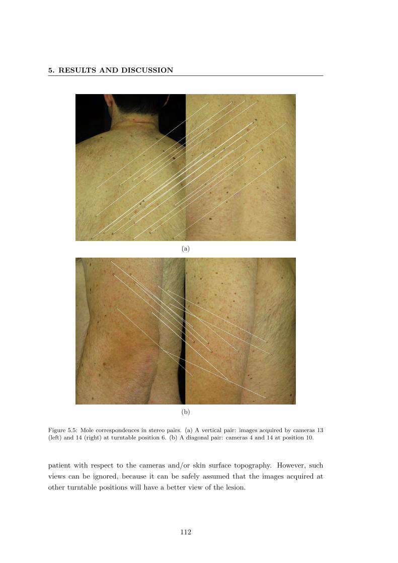
5. RESULTS AND DISCUSSION
(a)
(b)
Figure 5.5: Mole correspondences in stereo pairs. (a) A vertical pair: images acquired by cameras 13(left) and 14 (right) at turntable position 6. (b) A diagonal pair: cameras 4 and 14 at position 10.
patient with respect to the cameras and/or skin surface topography. However, such
views can be ignored, because it can be safely assumed that the images acquired at
other turntable positions will have a better view of the lesion.
112
5.1.5 PSL triangulation and mole set creation
Although the goal of the mole mapping is not to produce an accurate estimation of the
moles’ locations, but how well the system performs on average. The results of mole
triangulation can be evaluated with respect to repeatability (precision) and accuracy.
While the precision defines the consistency of the scanning system in estimating a
3D point’s location with different stereo pairs, the accuracy indicates how close these
estimations are to a real point. In order to determine these measures, we conducted two
experiments: (1) using 4384 visible markers in the calibration pattern and (2) 579 PSLs
detected in four explorations of two different patients. The first experiment included
the ground truth for the 3D points of the calibration board, which provided a basis
for the accuracy computation. For the PSL data of real patients, it is very difficult
to acquire such a ground truth, especially when taking into account the involuntary
movements during image acquisition.
In both experiments, we computed a number of unsigned distances between 3D
points and determined their means and standard deviations; for the accuracy, the dis-
tances between the estimated and real points, and for the precision, those between
triangulations produced by different stereo pairs for the same points/moles. Fig. 5.6
shows the probability density distributions describing the values obtained.3 The dia-
grams clearly demonstrate the difference in precision between the “synthetic” markers
in the pattern and the real mole points (the red lines). The standard deviation is three
times larger in the second experiment, with a mean precision 1.09 and 2.73 millimeters,
respectively. This is explained by the fact that the calibration markers are well defined
“corners” in space, so the detection noise has a much lower impact on the triangulation
precision. In contrast, real lesions are three-dimensional surfaces of different sizes pro-
jected onto the 2D planes of the sensors. The coordinates of their projections’ centroids
are dependent on the orientation of the lesions with respect to the cameras and the
accuracy of the blob detector. This inevitably leads to discrepancies in the 3D points
estimated.
The blue line in Fig. 5.6b confirms that it is practically impossible to obtain accurate
locations of the nevi on the patient’s body due to the use of a turntable. Nevertheless,
the precision shown by the algorithm in this experiment has the mean value of 5.55 mm
with a standard deviation of 3.9 mm. Together with the accuracy measured at µ = 3.24
mm with σ = 0.82, which was obtained on the “synthetic” data points (Fig. 5.6a), this
estimation is sufficient to approximately determine a PSL’s location on the body.
3Because the values are unsigned, the resulting Gaussians are not zero-centered.
113
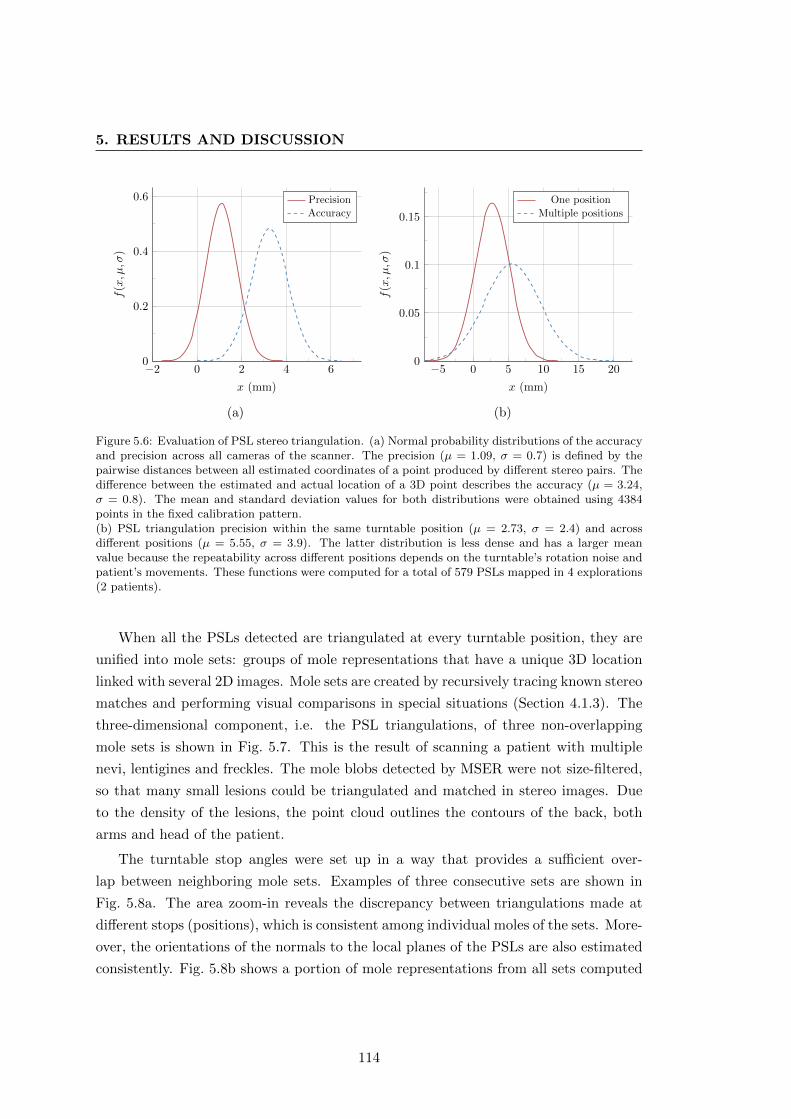
5. RESULTS AND DISCUSSION
−2 0 2 4 60
0.2
0.4
0.6
x (mm)
f(x, µ,σ
)
PrecisionAccuracy
(a)
−5 0 5 10 15 200
0.05
0.1
0.15
x (mm)f
(x, µ,σ
)
One position
Multiple positions
(b)
Figure 5.6: Evaluation of PSL stereo triangulation. (a) Normal probability distributions of the accuracyand precision across all cameras of the scanner. The precision (µ = 1.09, σ = 0.7) is defined by thepairwise distances between all estimated coordinates of a point produced by different stereo pairs. Thedifference between the estimated and actual location of a 3D point describes the accuracy (µ = 3.24,σ = 0.8). The mean and standard deviation values for both distributions were obtained using 4384points in the fixed calibration pattern.(b) PSL triangulation precision within the same turntable position (µ = 2.73, σ = 2.4) and acrossdifferent positions (µ = 5.55, σ = 3.9). The latter distribution is less dense and has a larger meanvalue because the repeatability across different positions depends on the turntable’s rotation noise andpatient’s movements. These functions were computed for a total of 579 PSLs mapped in 4 explorations(2 patients).
When all the PSLs detected are triangulated at every turntable position, they are
unified into mole sets: groups of mole representations that have a unique 3D location
linked with several 2D images. Mole sets are created by recursively tracing known stereo
matches and performing visual comparisons in special situations (Section 4.1.3). The
three-dimensional component, i.e. the PSL triangulations, of three non-overlapping
mole sets is shown in Fig. 5.7. This is the result of scanning a patient with multiple
nevi, lentigines and freckles. The mole blobs detected by MSER were not size-filtered,
so that many small lesions could be triangulated and matched in stereo images. Due
to the density of the lesions, the point cloud outlines the contours of the back, both
arms and head of the patient.
The turntable stop angles were set up in a way that provides a sufficient over-
lap between neighboring mole sets. Examples of three consecutive sets are shown in
Fig. 5.8a. The area zoom-in reveals the discrepancy between triangulations made at
different stops (positions), which is consistent among individual moles of the sets. More-
over, the orientations of the normals to the local planes of the PSLs are also estimated
consistently. Fig. 5.8b shows a portion of mole representations from all sets computed
114
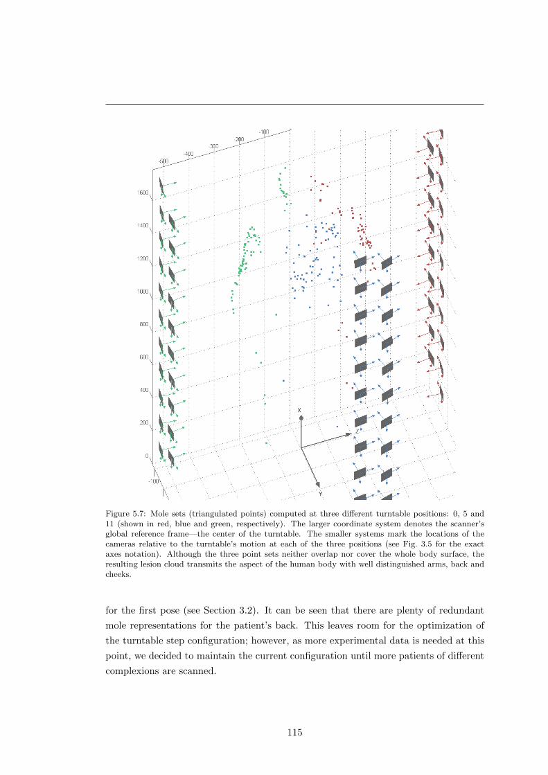
Figure 5.7: Mole sets (triangulated points) computed at three different turntable positions: 0, 5 and11 (shown in red, blue and green, respectively). The larger coordinate system denotes the scanner’sglobal reference frame—the center of the turntable. The smaller systems mark the locations of thecameras relative to the turntable’s motion at each of the three positions (see Fig. 3.5 for the exactaxes notation). Although the three point sets neither overlap nor cover the whole body surface, theresulting lesion cloud transmits the aspect of the human body with well distinguished arms, back andcheeks.
for the first pose (see Section 3.2). It can be seen that there are plenty of redundant
mole representations for the patient’s back. This leaves room for the optimization of
the turntable step configuration; however, as more experimental data is needed at this
point, we decided to maintain the current configuration until more patients of different
complexions are scanned.
115
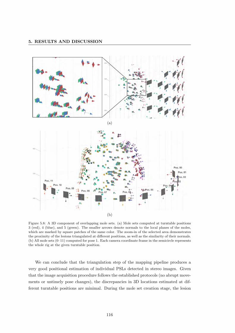
5. RESULTS AND DISCUSSION
(a)
(b)
Figure 5.8: A 3D component of overlapping mole sets. (a) Mole sets computed at turntable positions3 (red), 4 (blue), and 5 (green). The smaller arrows denote normals to the local planes of the moles,which are marked by square patches of the same color. The zoom-in of the selected area demonstratesthe proximity of the lesions triangulated at different positions, as well as the similarity of their normals.(b) All mole sets (0–11) computed for pose 1. Each camera coordinate frame in the semicircle representsthe whole rig at the given turntable position.
We can conclude that the triangulation step of the mapping pipeline produces a
very good positional estimation of individual PSLs detected in stereo images. Given
that the image acquisition procedure follows the established protocols (no abrupt move-
ments or untimely pose changes), the discrepancies in 3D locations estimated at dif-
ferent turntable positions are minimal. During the mole set creation stage, the lesion
116
representations (images and triangulations) obtained with the stereo pairs at every
turntable step are linked together. Essentially, these sets contain information about
PSLs visible to the cameras from a certain point of view (stop angle).
5.1.6 Mole set merging
In order to create a complete map of the PSLs on a patient’s body, the sets of mole
representations obtained at every turntable position must be merged together. The
merging is to be carried out separately for the two poses: turntable steps [0,11] and
[12,23]. For the moment, we have not considered merging the two resulting parts of a
full map, however, this will be addressed in future work (Section 6.4).
The mole set merging procedure uses the same principle of homography-based visual
comparison of individual lesions applied in stereo-pair matching (see Section 4.1.4). Due
to the fact that the images to be compared are not acquired simultaneously and the
patient is not absolutely still, we cannot rely on the epipolar geometry for the match
candidate selection. Instead, the Euclidean distance between moles’ triangulations is
used for the purpose. Images depicting moles are selected so that the difference in the
viewing angles is minimized, and the ROIs are transformed according to the known
camera geometry prior to extracting and matching the SIFT points.
Fig. 5.9 shows an example of a successful matching of mole representations at con-
secutive turntable positions. The lesion highlighted in Figs. 5.9a–c was photographed
by cameras installed on both columns, and has a different appearance in each image.
The view in Fig. 5.9c has the lowest η-metric because the lesion is most fronto-parallel
to camera 14 at position 5. In order to compare any two of the mole’s ROIs, one of
them is transformed using the fixed camera geometry to obtain roughly the same point
of view of the lesion as in the other ROI. Thus, Fig. 5.9d shows SIFT matches between
the transformed image (a) on the right and the original image (b) on the left. The lesion
was photographed at positions 3 and 4 respectively, making it a “p±1” matching case.
Likewise, in Fig. 5.9e, the “p± 2” candidates are matched, with image (a) transformed
accordingly (on the right).
Nevertheless, the visual comparison based on SIFT feature matches may fail in
certain cases. When the difference between the viewing angles of two images is too
sharp and the skin surface around a lesion is not planar, the SIFT points detected
will have dissimilar descriptors. Consequently, the result of SIFT-feature matching
will contain too many outliers, causing the homography estimation by RANSAC to be
unable to converge to a solution. An example of such a failure is shown in Fig. 5.10,
117
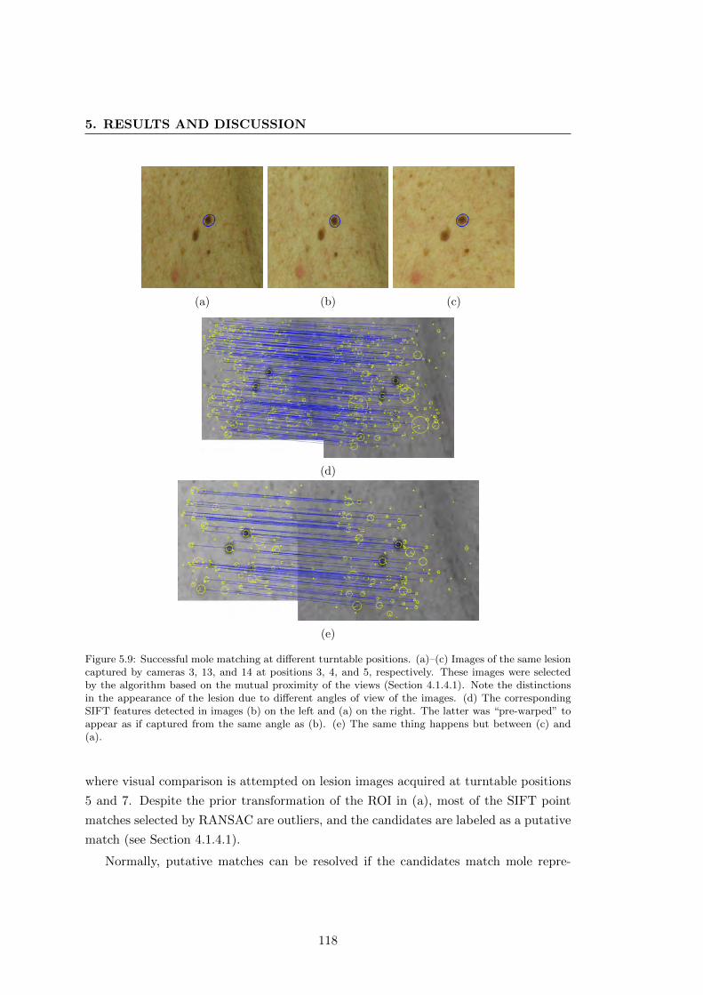
5. RESULTS AND DISCUSSION
(a) (b) (c)
(d)
(e)
Figure 5.9: Successful mole matching at different turntable positions. (a)–(c) Images of the same lesioncaptured by cameras 3, 13, and 14 at positions 3, 4, and 5, respectively. These images were selectedby the algorithm based on the mutual proximity of the views (Section 4.1.4.1). Note the distinctionsin the appearance of the lesion due to different angles of view of the images. (d) The correspondingSIFT features detected in images (b) on the left and (a) on the right. The latter was “pre-warped” toappear as if captured from the same angle as (b). (e) The same thing happens but between (c) and(a).
where visual comparison is attempted on lesion images acquired at turntable positions
5 and 7. Despite the prior transformation of the ROI in (a), most of the SIFT point
matches selected by RANSAC are outliers, and the candidates are labeled as a putative
match (see Section 4.1.4.1).
Normally, putative matches can be resolved if the candidates match mole repre-
118
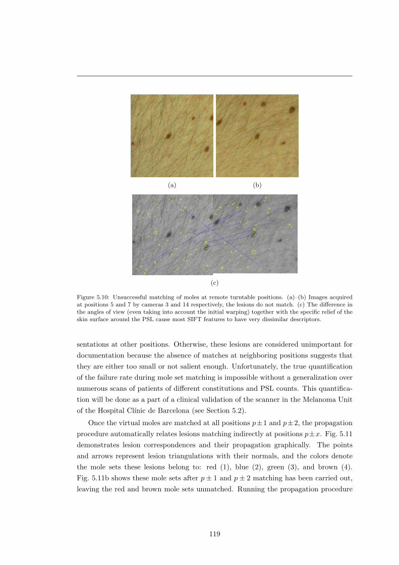
(a) (b)
(c)
Figure 5.10: Unsuccessful matching of moles at remote turntable positions. (a)–(b) Images acquiredat positions 5 and 7 by cameras 3 and 14 respectively, the lesions do not match. (c) The difference inthe angles of view (even taking into account the initial warping) together with the specific relief of theskin surface around the PSL cause most SIFT features to have very dissimilar descriptors.
sentations at other positions. Otherwise, these lesions are considered unimportant for
documentation because the absence of matches at neighboring positions suggests that
they are either too small or not salient enough. Unfortunately, the true quantification
of the failure rate during mole set matching is impossible without a generalization over
numerous scans of patients of different constitutions and PSL counts. This quantifica-
tion will be done as a part of a clinical validation of the scanner in the Melanoma Unit
of the Hospital Clınic de Barcelona (see Section 5.2).
Once the virtual moles are matched at all positions p±1 and p±2, the propagation
procedure automatically relates lesions matching indirectly at positions p±x. Fig. 5.11
demonstrates lesion correspondences and their propagation graphically. The points
and arrows represent lesion triangulations with their normals, and the colors denote
the mole sets these lesions belong to: red (1), blue (2), green (3), and brown (4).
Fig. 5.11b shows these mole sets after p± 1 and p± 2 matching has been carried out,
leaving the red and brown mole sets unmatched. Running the propagation procedure
119
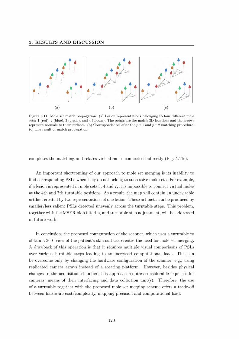
5. RESULTS AND DISCUSSION
(a) (b) (c)
Figure 5.11: Mole set match propagation. (a) Lesion representations belonging to four different molesets: 1 (red), 2 (blue), 3 (green), and 4 (brown). The points are the mole’s 3D locations and the arrowsrepresent normals to their surfaces. (b) Correspondences after the p± 1 and p± 2 matching procedure.(c) The result of match propagation.
completes the matching and relates virtual moles connected indirectly (Fig. 5.11c).
An important shortcoming of our approach to mole set merging is its inability to
find corresponding PSLs when they do not belong to successive mole sets. For example,
if a lesion is represented in mole sets 3, 4 and 7, it is impossible to connect virtual moles
at the 4th and 7th turntable positions. As a result, the map will contain an undesirable
artifact created by two representations of one lesion. These artifacts can be produced by
smaller/less salient PSLs detected unevenly across the turntable steps. This problem,
together with the MSER blob filtering and turntable step adjustment, will be addressed
in future work
In conclusion, the proposed configuration of the scanner, which uses a turntable to
obtain a 360° view of the patient’s skin surface, creates the need for mole set merging.
A drawback of this operation is that it requires multiple visual comparisons of PSLs
over various turntable steps leading to an increased computational load. This can
be overcome only by changing the hardware configuration of the scanner, e.g., using
replicated camera arrays instead of a rotating platform. However, besides physical
changes to the acquisition chamber, this approach requires considerable expenses for
cameras, means of their interfacing and data collection unit(s). Therefore, the use
of a turntable together with the proposed mole set merging scheme offers a trade-off
between hardware cost/complexity, mapping precision and computational load.
120
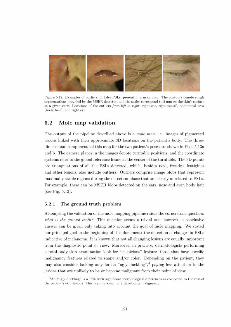
Figure 5.12: Examples of outliers, or false PSLs, present in a mole map. The contours denote roughsegmentations provided by the MSER detector, and the scales correspond to 5 mm on the skin’s surfaceat a given view. Locations of the outliers from left to right : right ear, right nostril, abdominal area(body hair), and right eye.
5.2 Mole map validation
The output of the pipeline described above is a mole map, i.e. images of pigmented
lesions linked with their approximate 3D locations on the patient’s body. The three-
dimensional components of this map for the two patient’s poses are shown in Figs. 5.13a
and b. The camera planes in the images denote turntable positions, and the coordinate
systems refer to the global reference frame at the center of the turntable. The 3D points
are triangulations of all the PSLs detected, which, besides nevi, freckles, lentigines
and other lesions, also include outliers. Outliers comprise image blobs that represent
maximally stable regions during the detection phase that are clearly unrelated to PSLs.
For example, these can be MSER blobs detected on the ears, nose and even body hair
(see Fig. 5.12).
5.2.1 The ground truth problem
Attempting the validation of the mole mapping pipeline raises the cornerstone question:
what is the ground truth? This question seems a trivial one, however, a conclusive
answer can be given only taking into account the goal of mole mapping. We stated
our principal goal in the beginning of this document: the detection of changes in PSLs
indicative of melanoma. It is known that not all changing lesions are equally important
from the diagnostic point of view. Moreover, in practice, dermatologists performing
a total-body skin examination look for “suspicious” lesions: those that have specific
malignancy features related to shape and/or color. Depending on the patient, they
may also consider looking only for an “ugly duckling”,4 paying less attention to the
lesions that are unlikely to be or become malignant from their point of view.
4An “ugly duckling” is a PSL with significant morphological differences as compared to the rest ofthe patient’s skin lesions. This may be a sign of a developing malignancy.
121
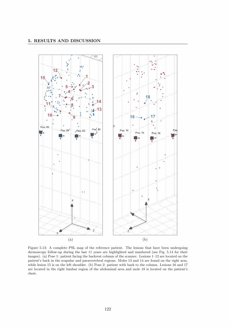
5. RESULTS AND DISCUSSION
(a) (b)
Figure 5.13: A complete PSL map of the reference patient. The lesions that have been undergoingdermoscopy follow-up during the last 11 years are highlighted and numbered (see Fig. 5.14 for theirimages). (a) Pose 1: patient facing the backrest column of the scanner. Lesions 1–12 are located on thepatient’s back in the scapular and paravertebral regions. Moles 13 and 14 are found on the right arm,while lesion 15 is on the left shoulder. (b) Pose 2: patient with back to the column. Lesions 16 and 17are located in the right lumbar region of the abdominal area and mole 18 is located on the patient’schest.
122
Consequently, we are discussing a restriction on the total body skin examination
to the lesions considered relevant. This is a rational approach which saves time in
the presence of numerous nevi; however, the definition of relevance is rather subjective
and can vary from physician to physician. Relevant lesions may also include different
types of PSLs depending on the patient’s history and risk factors. For example, in
some patients, a physician will bias the screening to dysplastic nevi, while in others,
lentigines will be of interest too. As a result, lesions irrelevant from the point of view
of a dermatologist are ignored during the examination, and their evolution over time is
not closely followed.5 In most cases, these skipped lesions do not have any malignancy
potential. However, a manual PSL screening influenced, in addition, by subjective
criteria leaves room for human error.
From this point, we can see that there is no general unambiguous answer to the
ground truth question. Nevertheless, at the current stage of the scanner’s development,
we can specify the minimum results the mapping is expected to produce. In particular,
an exploration map should contain all lesions considered relevant by dermatologists for a
specific patient, as well as those satisfying some appearance criteria. Without additional
filtering (e.g. based on machine learning), the appearance criteria are conditioned only
by the scanner’s camera system and the skin-to-lesion contrast. The camera resolution
restricts the size of observable PSLs, while low-contrast lesions are discarded to avoid
cluttering the map. Having more than relevant lesions in the map reduces the risk of
missing PSLs that can potentially lead to a malignancy.
Thus, in order to comprehensively evaluate the performance of the PSL mapping, we
need to have the ground truth of the patient’s lesions which are considered relevant by
several dermatologists. In clinical practice, such data collection requires combining both
a manual TBSE procedure and an automated exploration using the scanner prototype.
Therefore, the scanner was recently installed in the Melanoma Unit of the Hospital
Clınic de Barcelona for clinical validation under the supervision of Dr. Josep Malvehy
and Dr. Susanna Puig.
5.2.2 Preliminary evaluation
For evaluation of the algorithms’ performance in a laboratory setting, we used the total
body examination history available for one of our volunteer patients. This history data
5In this respect, there is an important conceptual advantage with our scanner. If a lesion that wasnot detected previously is detected during the latest scan, it is possible to verify whether this is a resultof its evolution over time or was simply missed before. By tracking only relevant lesions, as currentlypracticed in TBSE, this verification is impossible.
123
5. RESULTS AND DISCUSSION
included dermoscopy (MoleMax�) and clinical images of several PSLs undergoing regu-
lar monitoring over the last 11 years. During this period, the patient was examined by
several dermatologists trained in dermoscopy, and the images were acquired by different
technicians. The clinical photographs comprise only low-resolution macroscopic images
of the patient in standardized poses (see Section 1.4.1.1), while the high-resolution
dermoscopy images were used for the analysis and temporal monitoring of the lesions.
Hence, the PSLs subject to dermoscopy follow-up were qualified as the relevant lesion
ground truth for that patient.
We selected a total of 17 lesions in the areas visible by the scanner’s cameras6 and
not completely occluded by body hair. The moles undergoing dermoscopy follow-up
were found in the paravertebral and scapular regions, as well as on the right arm,
left shoulder and chest (Fig. 5.13). As shown in Figs. 5.13 and 5.14, all these lesions
were successfully mapped by the scanner. The side-by-side views of the clinical and
corresponding dermoscopic images of the moles are shown in the latter figure. Although
the level of detail offered by the images of different types is incomparable, the scanner’s
photographs can be well used for the detection of changes in the lesions’ shape and
color.
While the lesions in the clinical photographs have the same global orientation,7
their orientations in the dermoscopic images are arbitrary. We deliberately left them
unaltered in order to demonstrate the difficulty of establishing lesion-to-image corre-
spondences manually (see also Fig. 1.6 in Section 1.5). In addition, one of the lesions
examined in the chest region (#18), heavily occluded by body hair, was mapped by
the scanner as well. However, due to the hair occlusion, it cannot be used in automatic
change detection.
The results of the preliminary evaluation do not give a definitive assessment of the
mole mapping pipeline. Nevertheless, they provide valuable information that will help
to anticipate and improve the performance of the algorithms in future clinical trials.
Thus, the following conclusions of this validation can be highlighted:
� In a larger trial, we strive to achieve the same results regarding the sensitivity:
in the test patient, 100% of the lesions considered relevant were mapped.
� The repeatability of mapping smaller/less salient lesions (freckles and lentigines)
should be improved: on average, 7–10 PSLs mapped in one exploration were
missed in other scans. In total, 208–222 lesions (the minimum and maximum
6The lesions found on the soles, the palms and the scalp were not taken into account.7The vertical dimension of the images coincides with the vertical axis of the scanner.
124
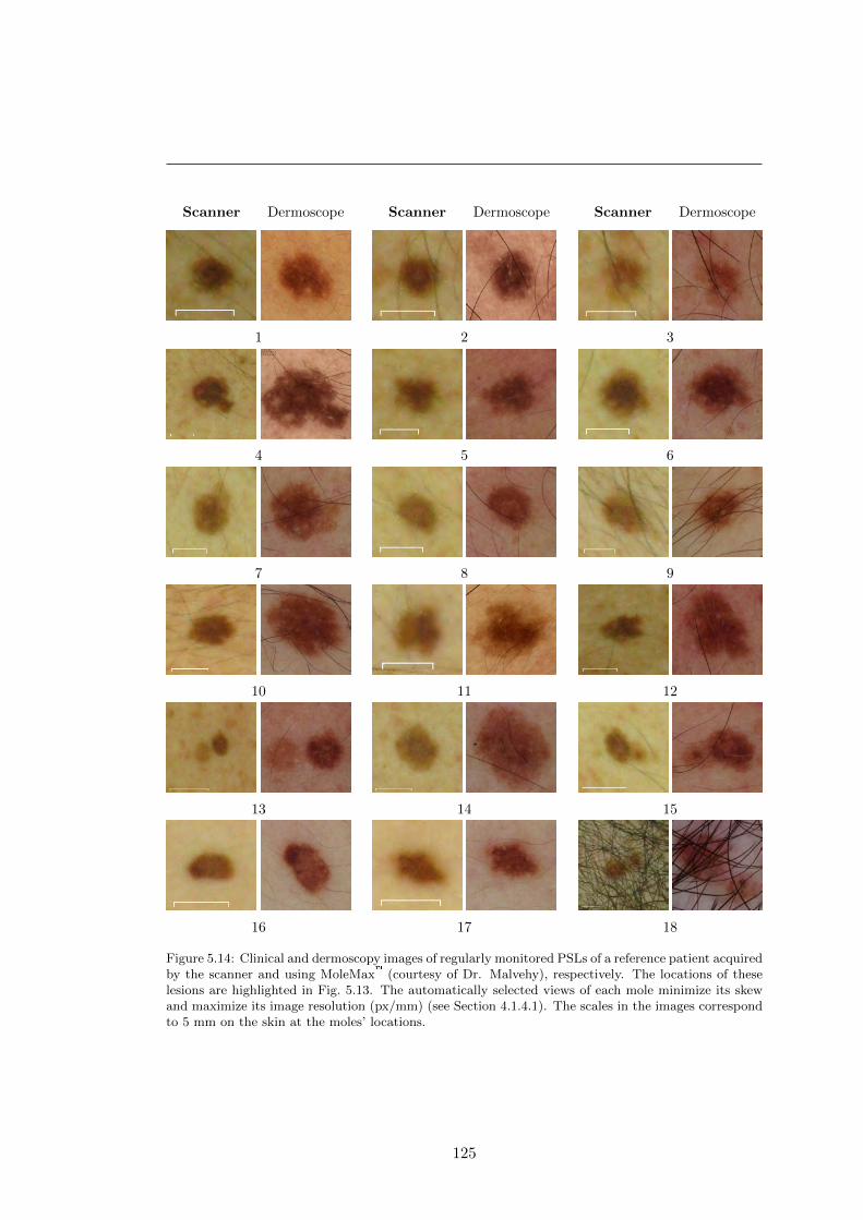
Scanner Dermoscope
1
Scanner Dermoscope
2
Scanner Dermoscope
3
4 5 6
7 8 9
10 11 12
13 14 15
16 17 18
Figure 5.14: Clinical and dermoscopy images of regularly monitored PSLs of a reference patient acquiredby the scanner and using MoleMax� (courtesy of Dr. Malvehy), respectively. The locations of theselesions are highlighted in Fig. 5.13. The automatically selected views of each mole minimize its skewand maximize its image resolution (px/mm) (see Section 4.1.4.1). The scales in the images correspondto 5 mm on the skin at the moles’ locations.
125
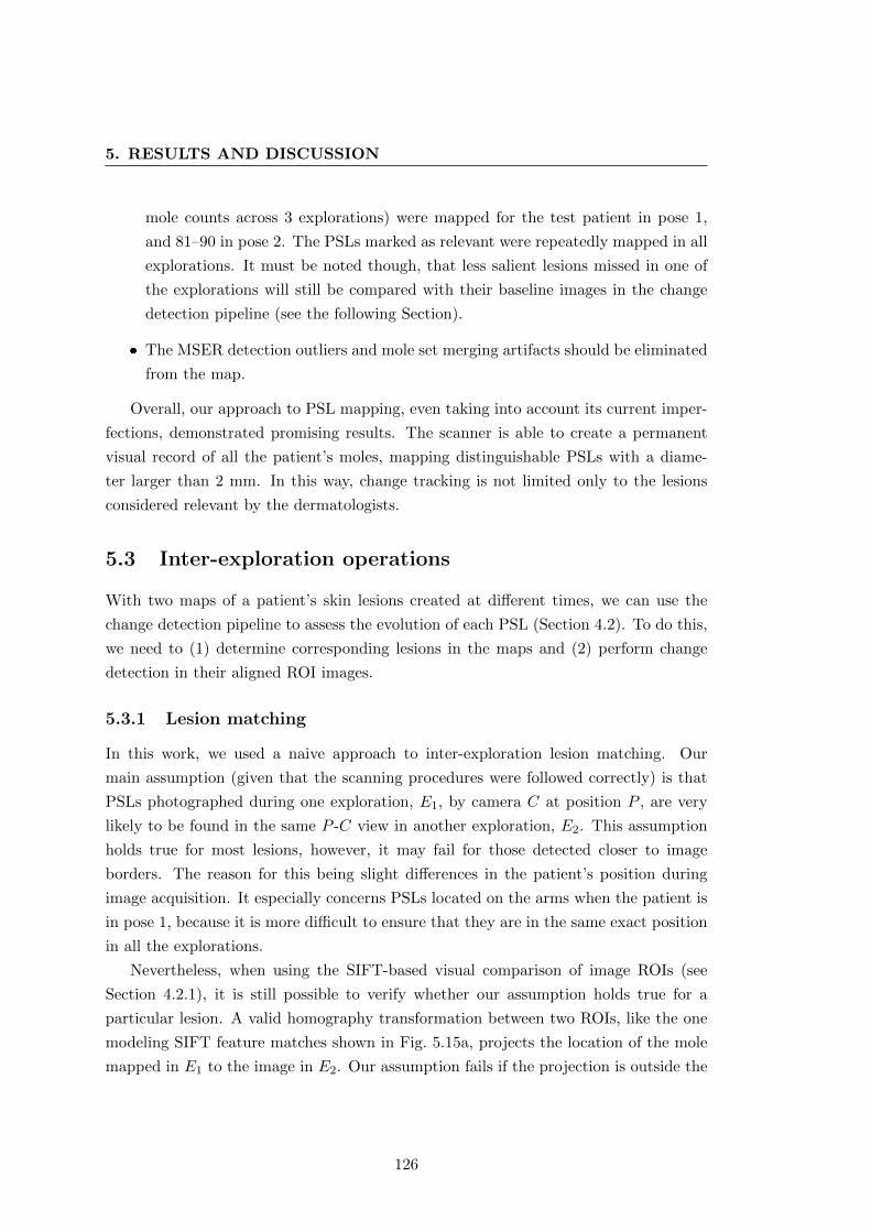
5. RESULTS AND DISCUSSION
mole counts across 3 explorations) were mapped for the test patient in pose 1,
and 81–90 in pose 2. The PSLs marked as relevant were repeatedly mapped in all
explorations. It must be noted though, that less salient lesions missed in one of
the explorations will still be compared with their baseline images in the change
detection pipeline (see the following Section).
� The MSER detection outliers and mole set merging artifacts should be eliminated
from the map.
Overall, our approach to PSL mapping, even taking into account its current imper-
fections, demonstrated promising results. The scanner is able to create a permanent
visual record of all the patient’s moles, mapping distinguishable PSLs with a diame-
ter larger than 2 mm. In this way, change tracking is not limited only to the lesions
considered relevant by the dermatologists.
5.3 Inter-exploration operations
With two maps of a patient’s skin lesions created at different times, we can use the
change detection pipeline to assess the evolution of each PSL (Section 4.2). To do this,
we need to (1) determine corresponding lesions in the maps and (2) perform change
detection in their aligned ROI images.
5.3.1 Lesion matching
In this work, we used a naive approach to inter-exploration lesion matching. Our
main assumption (given that the scanning procedures were followed correctly) is that
PSLs photographed during one exploration, E1, by camera C at position P , are very
likely to be found in the same P -C view in another exploration, E2. This assumption
holds true for most lesions, however, it may fail for those detected closer to image
borders. The reason for this being slight differences in the patient’s position during
image acquisition. It especially concerns PSLs located on the arms when the patient is
in pose 1, because it is more difficult to ensure that they are in the same exact position
in all the explorations.
Nevertheless, when using the SIFT-based visual comparison of image ROIs (see
Section 4.2.1), it is still possible to verify whether our assumption holds true for a
particular lesion. A valid homography transformation between two ROIs, like the one
modeling SIFT feature matches shown in Fig. 5.15a, projects the location of the mole
mapped in E1 to the image in E2. Our assumption fails if the projection is outside the
126
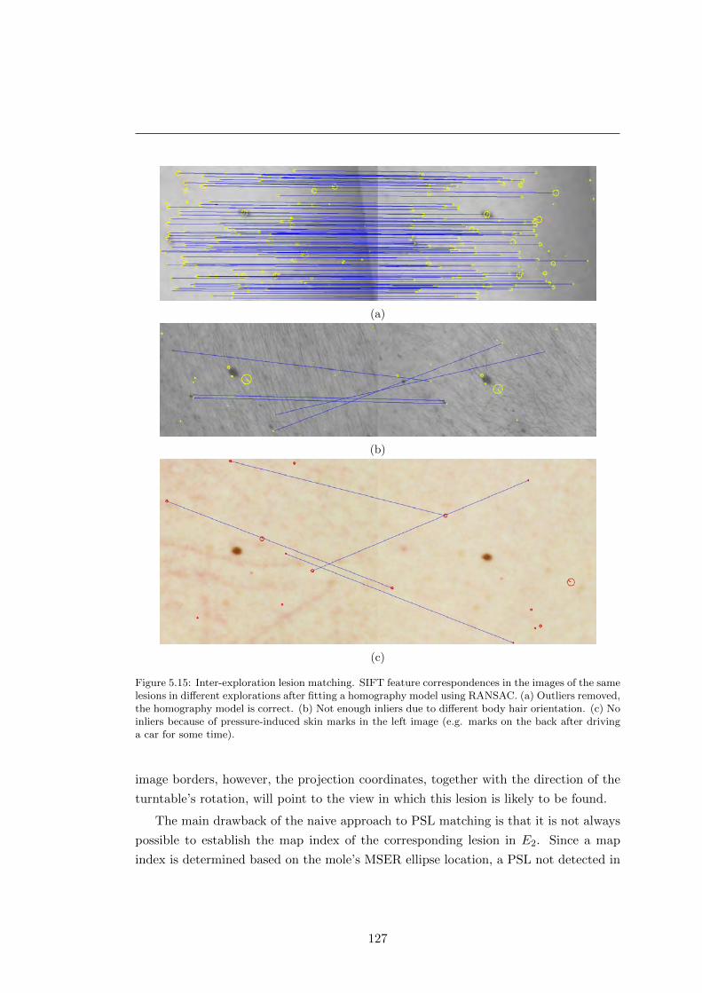
(a)
(b)
(c)
Figure 5.15: Inter-exploration lesion matching. SIFT feature correspondences in the images of the samelesions in different explorations after fitting a homography model using RANSAC. (a) Outliers removed,the homography model is correct. (b) Not enough inliers due to different body hair orientation. (c) Noinliers because of pressure-induced skin marks in the left image (e.g. marks on the back after drivinga car for some time).
image borders, however, the projection coordinates, together with the direction of the
turntable’s rotation, will point to the view in which this lesion is likely to be found.
The main drawback of the naive approach to PSL matching is that it is not always
possible to establish the map index of the corresponding lesion in E2. Since a map
index is determined based on the mole’s MSER ellipse location, a PSL not detected in
127
5. RESULTS AND DISCUSSION
a particular image will be untraceable. On the other hand, this approach will succeed in
performing change detection even though the lesion in E1 is not mapped in E2 because
it will still be present in both images. Therefore, in order to produce stable map index
matches as well as account for missing lesions, the naive approach can be combined
with a more sophisticated technique, e.g. based on a non-rigid point cloud registration.
This will be addressed in future work.
The estimation of a homography between two skin image patches can fail if the
images have completely different gradient information. This will lead to a proportion
of false feature correspondences that the RANSAC algorithm is unable to filter out. In
our experiments, we have determined two situations causing such behavior:
1. Body hair in the image patches with different orientations, Fig. 5.15b.
2. Presence of pressure-induced skin marks in one of the images, Fig. 5.15c.
As the figures demonstrate, the RANSAC algorithm was not able to estimate a correct
homography model, because the percentage of SIFT match outliers is too high. Conse-
quently, as these results suggest, the scanning procedure should be limited to patients
with no or little body hair, and any skin alteration that drastically changes its image
gradient information should be avoided.
5.3.2 Change detection
After applying a homography to align the images and refine this alignment by means of
normalized cross-correlation, we can obtain a difference image of the two skin images.
Figs. 5.16a–d show image patches of moles that did not evolve between explorations.
The respective change maps in Figs. 5.16a, b and d, nevertheless, contain artifacts
(clusters of black pixels) that correspond to alignment inaccuracies, sensor noise and
body hair influence. Such artifacts do not produce false change alerts as they are
filtered out by thresholding the ratio of their total area to the union area of the two
lesion segmentations (see Section 4.2.2).
Because our experiments were conducted using limited data, we modified some of
the patients’ lesions and added new moles using color markers. The newly appearing
“lesions” are shown in Figs. 5.16e–f. The difference images masked by the coarse MSER
segmentations indicate a 100% change. In other words, it can be automatically deter-
mined that the lesion was not there during the previous exploration. This demonstrates
that the scanner is capable of early detection of small (less than 3 mm) new lesions.
Examples of the detection of artificial changes are shown in Figs. 5.16g–j. Real
changes, in most cases, may not have as high a contrast between the skin and lesion
128
Map1 Map2 Change
(a)
Map1 Map2 Change
(b)
(c) (d)
(e) (f)
(g) (h)
(i) (j)
Figure 5.16: The detection of new and evolving (synthetic) skin lesions. In each subfigure, the imagesare ordered from left to right: lesion view in the 1st exploration, transformed view in the 2nd explorationand the change map. The scales correspond to 5 mm on the skin’s surface at the lesions’ location. (a)–(d) Lesions without any evolution. (e)–(f) Newly appeared artificial “moles”. (g)–(j) PSLs with changesadded using black and red markers.
texture. Nevertheless, these approximations can give an idea of the scale at which
the changes can be easily detected. In Fig. 5.16h, the segmentations of the lesion are
fairly inaccurate, and can potentially lead to missed changes. Therefore, besides the
global MSER detection/segmentation, it may be useful to apply additional algorithms
for refining the border delineation.
129
5. RESULTS AND DISCUSSION
Due to the use of an HSV color space, subtle differences, such as the artificial red-
dening in Fig. 5.16i, can be easily spotted. Of course, this can also produce false positive
changes due to sensor noise or illumination inconsistencies caused by the camera-to-
skin-surface angle. However, the actual influence of the noise on change detection can
be fully analyzed after a much wider validation on real changing lesions. It must also be
noted that the current approach does not take into account skin tan variations between
images acquired in different seasons. In order to account for such differences, we will
need to build an appropriate illumination model based on future exploration data.
Overall, Fig. 5.16 demonstrates the ability of the skin scanner to automatically de-
tect new and evolving lesions between explorations, although, for now, just on synthetic
examples. The initial experimental material, gathered during the validation of all the
steps in the mapping and change detection pipelines, highlights both advantages and
drawbacks of our approach, suggesting ways to improve the algorithms. This is further
discussed in the next and concluding chapter of this thesis.
130
Chapter 6
Conclusions
Ever since the first description of melanoma as a disease entity in 1806 [8], science has
been trying to find efficient ways to fight this dangerous malignancy. As a consequence,
numerous important findings about the nature and features of this cancer have been
made and have led to the elaboration of various methodologies to recognize melanoma
as well as the creation of its core treatment philosophy: excision as early as possible.
Adhering to this philosophy, dermatologists seek reliable visual signs that would
indicate an early melanoma in order to remove it safely and eliminate any chance of
cancerous spreading. However, the appearance of pigmented skin lesions, the precursors
of melanoma, can be exceptionally misleading and renders lesion feature interpretation a
particularly difficult task whose outcome greatly depends on the professional experience
of the physician. Moreover, the most advanced state-of-the-art artificial intelligence
systems cannot as yet outperform human experts.
Nevertheless, there is an alternative way in which computer vision can significantly
contribute to the timely detection of melanoma. A factor which is widely acknowl-
edged to be indicative of a developing deadly malignancy is rapid evolution of or some
change in pigmented lesions. This change may be hard to perceive with the naked
eye, especially since the term “rapid” normally refers to a period of 3 to 6 months.
Consequently, during a patient’s examination, physicians rely on baseline photography
and an unaided visual search for lesions that could have evolved since the previous
check-up. It is not difficult to imagine the amount of work and error risk involved
when examining a patient with dozens of atypical moles exhibiting ambiguous features.
Moreover, the recognition and localization of lesions depicted in baseline photographs
can be extremely time-consuming.
Hence, it is clear that the automation of routine TBSE/TBSI procedures can save
131
6. CONCLUSIONS
time and resources, reduce patient morbidity, and minimize potential detection errors.
For this reason, we have carefully reviewed the literature related to the application
of computer vision to diagnosing melanoma. Our review showed that throughout the
entire history of the field, change detection has not received due attention, and few
attempts have been made to automate the multiple lesion analysis. This important
finding gave us motivation to develop a tool for TBSE automation as well as attract
more attention to the problem of automatic change detection in PSLs.
6.1 Summary of the thesis
We started our research by studying the intersection area of computer vision with
the part of dermatology concerned with malignancies developing from pigmented skin
lesions. The introduction chapter briefly presented the medical aspects of the field
clarifying ambiguities in terminology and explaining in detail the motivation behind
this work. In particular, it described the structure of the human skin and the main
types of cells present in the cutis, gaving basic information about benign PSLs that
are known to be precursors of melanoma, and outlining the imaging techniques and
diagnosis methodologies used to detect this deadly cancer. We highlighted the fact
that a primordial role in detecting a developing melanoma is played by a total body
skin examination, and that its automation has not received due attention.
Chapter 2 extended this study by an in-depth review of the literature addressing
the computerized analysis of PSL images (micro- and macroscopic) aimed at diagnosing
melanoma. We classified the existing literature according to the nature of publication
(clinical or computer vision articles) differentiating between individual and multiple
PSL image analysis. Relevant references were categorized, emphasizing the impor-
tance of the difference in content between dermoscopic and clinical images. Various
approaches for implementing PSL computer-aided diagnosis systems and their stan-
dard workflow components were reviewed and summary tables provided. Based on the
conclusions drawn from this review, we directed our work towards the development of
a strategy aimed at the automation of TBSE/TBSI procedures.
In Chapter 3, we described a new total body skin scanning system designed and
built in-house (briefly presented in [15] for the first time). This chapter dwells on the
system’s hardware including the imaging module, operation concept and the calibration
procedure. The scanner allows for the acquisition of a series of overlapping cross-
polarized high-resolution images covering 85-90% of the patient’s skin surface. In order
to process these images and use their content for change detection in multiple nevi, we
132
have developed a set of computer vision algorithms described in Chapter 4.
Instead of performing a complete reconstruction of the patient’s skin surface (this
is practically possible), our strategy consisted of binding locations of individual PSLs
with their images acquired by means of the scanner. Thus, after each exploration, the
lesions are detected in the images, matched across stereo pairs at different positions
of the turntable and grouped into sets. Merging these sets into a mole map creates a
topological description of all visible PSLs on the patient’s body. Using the controlled
environment of the acquisition chamber and following the scanning protocol, two such
maps from different scans can be matched, and temporal changes in individual lesions
detected. The results of a successful application of these algorithms to the real image
sets are reported in Chapter 5.
6.2 Contributions
The following are the major contributions of this thesis:
� A set of algorithms used in conjunction with a total body skin scanner that
automatically solve two important TBSE problems:
– Lesion-to-image and image-to-lesion correspondence: localize the PSL on
the patient’s body given its image, and vice versa.
– Inter-exploration lesion correspondence: match an image of a PSL acquired
during examination 1 to the image of the same lesion after examination 2.
As a result, the scanner is able to assist in routine TBSE procedures and auto-
matically select lesions that require a closer analysis due to changes they have
undergone since the baseline examination. It allows verification of the previous
state of any PSL, and not just those considered relevant by a dermatologist during
a previous examination. This is the first research work proposing a complete solu-
tion (software- and hardware-wise) for the problem of automatic change detection
in multiple PSLs.
� An in-depth literature review spanning publications from over 20 years of research
in the field of computerized analysis of PSLs. The review demonstrated a large
discrepancy in the number of articles published on individual and multiple PSL
image analysis and a scarcity of reported material on the automation of lesion
change detection. Furthermore, we proposed an extended categorization of PSL
133

6. CONCLUSIONS
feature descriptors, associating them with the specific methods for diagnosing
melanoma and separating images of the two modalities.
� A method for pattern assembly using several unique squares and one separator
square: the “abacus encoding scheme”. The internal corners of the resulting
pattern hold a unique signature conditioned by the four surrounding squares.
The scheme was used to design the color-coded pattern for a one-shot external
calibration of the scanner’s camera rig.
6.3 Limitations
Any device has its limitations, and the total body skin scanner presented is no ex-
ception. The nature of the algorithms and the hardware design establishes 2 main
shortcomings:
� Body hair restriction. Due to the properties of the SIFT detector, which, in
this case, relies heavily on the skin texture, patients undergoing the scanning
procedure should have as little body hair as possible. Although the mole mapping
pipeline will perform as expected even in the presence of thick hair, the inter-
exploration mole matching may fail because of an alteration in their orientation.1
Such an alteration results in a change of skin texture, which in turn leads to a
significant dissimilarity of the SIFT points detected in the images from different
explorations. Therefore, ideally, body hair should be completely removed before
the examination.
� Unreachable body regions. The two poses assumed by the patient during the
scanning procedure leave some areas unobserved: the soles of the feet, the palms
of the arms, the inner surface of the arms, the scalp and the area behind the
ears. For a complete TBSE, these areas should be photographed and analyzed
separately.
6.4 Further work
The main directions for further work can be viewed in short-term and long-term per-
spectives. The short-term goals include:
1This may happen when changing clothes, for example.
134

� Continuous validation of the scanner’s hardware and software in a real clinical
setting. This stage is vital for discovering potential weak points in the approach,
correcting exiting errors (”debugging”) and fine-tunning the parameters.
� Various algorithm improvements: removal of the mole set merging artifacts, en-
hancement of the inter-exploration lesion matching (naive approach + point cloud
registration) and refinement of rough MSER segmentations.
� Merging the mole maps for the two poses. Some of the lesions mapped when the
patient is in pose 1 will overlap with those acquired at pose 2, for example PSLs
on the shoulders and cheeks. A unified representation of the map for the whole
body will reduce unnecessary redundancy and facilitate data interpretation for
physicians.
� PSL classification. Apart from the nevi, interesting from the point of view of
melanoma diagnosis, the output of the mole detection may contain other “blobs”.
For example, lesions of similar appearance, such as freckles or acne, or even non-
lesion spots, e.g. nostrils or ear convolutions, can be detected as PSLs. They
produce noise in the output of the change detection pipeline as well as waste
computational resources, and thus should be discarded in earlier stages. One
possible way to do this is by applying a binary classifier to the detected blobs,
which, based on certain features, can determine whether these blobs represent a
PSL of interest or not. The research alone needed to obtain such a classifier forms
some serious scientific work.
Among the long-term work directions we can highlight the following:
� Improve camera focusing. In the presented scanning system, the focusing in some
images is clearer that in others. This is conditioned by the fact that the focus
distance is fixed throughout the entire exploration, while the space between the
body and the cameras varies. Consequently, the established depth of field of the
cameras is not enough to account for the difference. This can be overcome by em-
ploying an external focusing aid (e.g. ultrasonic sensors) or using cameras/optics
allowing for a more flexible tuning. In either case, simultaneous image acquisition
by all the cameras must be preserved.
� Improve camera resolution. In order to perform a more minute analysis and catch
the smallest change in a PSL, the image resolution should be increased (currently,
the cameras acquire 12-megapixel images). As a side effect, this will increase the
135

6. CONCLUSIONS
amount of image data as well and affect the performance of the algorithms, so
the data handling procedures must be changed accordingly.
� Change characterization. Given the higher-resolution images with improved fo-
cusing, we can work out strategies for detailed automatic change characterization.
Since lesions change not only in size, but also in color and morphology, the scan-
ning system may be used to better study the character of changes in malignant
growths.
136
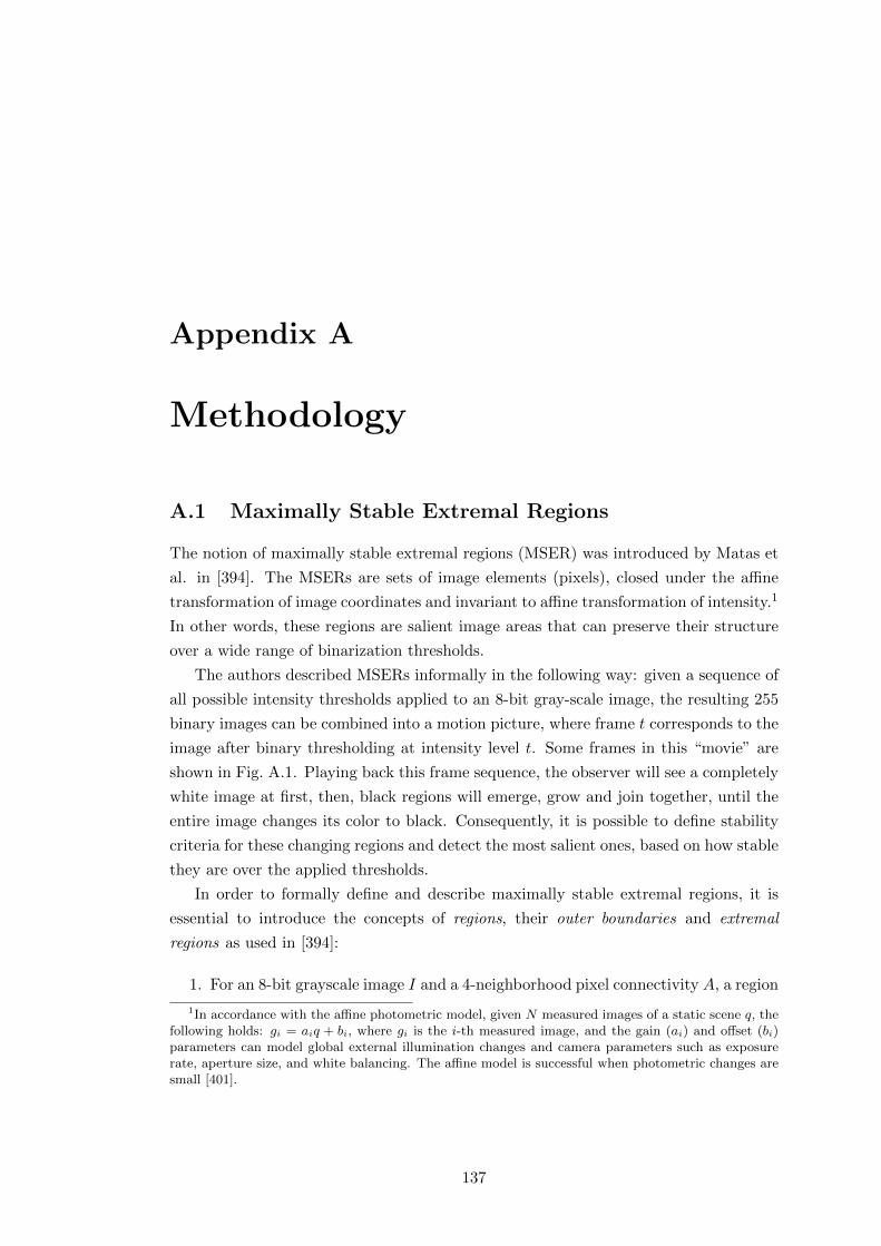
Appendix A
Methodology
A.1 Maximally Stable Extremal Regions
The notion of maximally stable extremal regions (MSER) was introduced by Matas et
al. in [394]. The MSERs are sets of image elements (pixels), closed under the affine
transformation of image coordinates and invariant to affine transformation of intensity.1
In other words, these regions are salient image areas that can preserve their structure
over a wide range of binarization thresholds.
The authors described MSERs informally in the following way: given a sequence of
all possible intensity thresholds applied to an 8-bit gray-scale image, the resulting 255
binary images can be combined into a motion picture, where frame t corresponds to the
image after binary thresholding at intensity level t. Some frames in this “movie” are
shown in Fig. A.1. Playing back this frame sequence, the observer will see a completely
white image at first, then, black regions will emerge, grow and join together, until the
entire image changes its color to black. Consequently, it is possible to define stability
criteria for these changing regions and detect the most salient ones, based on how stable
they are over the applied thresholds.
In order to formally define and describe maximally stable extremal regions, it is
essential to introduce the concepts of regions, their outer boundaries and extremal
regions as used in [394]:
1. For an 8-bit grayscale image I and a 4-neighborhood pixel connectivity A, a region
1In accordance with the affine photometric model, given N measured images of a static scene q, thefollowing holds: gi = aiq + bi, where gi is the i-th measured image, and the gain (ai) and offset (bi)parameters can model global external illumination changes and camera parameters such as exposurerate, aperture size, and white balancing. The affine model is successful when photometric changes aresmall [401].
137
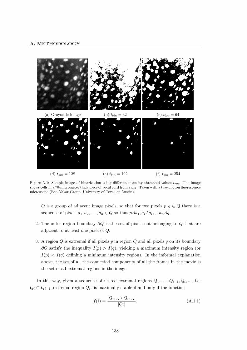
A. METHODOLOGY
(a) Grayscale image (b) tbin = 32 (c) tbin = 64
(d) tbin = 128 (e) tbin = 192 (f) tbin = 254
Figure A.1: Sample image of binarization using different intensity threshold values tbin. The imageshows cells in a 70-micrometer thick piece of vocal cord from a pig. Taken with a two-photon fluorescencemicroscope (Ben-Yakar Group, University of Texas at Austin).
Q is a group of adjacent image pixels, so that for two pixels p, q ∈ Q there is a
sequence of pixels a1, a2, . . . , an ∈ Q so that pAa1, aiAai+1, anAq.
2. The outer region boundary ∂Q is the set of pixels not belonging to Q that are
adjacent to at least one pixel of Q.
3. A region Q is extremal if all pixels p in region Q and all pixels q on its boundary
∂Q satisfy the inequality I(p) > I(q), yielding a maximum intensity region (or
I(p) < I(q) defining a minimum intensity region). In the informal explanation
above, the set of all the connected components of all the frames in the movie is
the set of all extremal regions in the image.
In this way, given a sequence of nested extremal regions Q1, . . . , Qi−1, Qi, ..., i.e.
Qi ⊂ Qi+1, extremal region Qi∗ is maximally stable if and only if the function
f(i) =|Qi+∆ \Qi−∆|
|Qi|, (A.1.1)
138
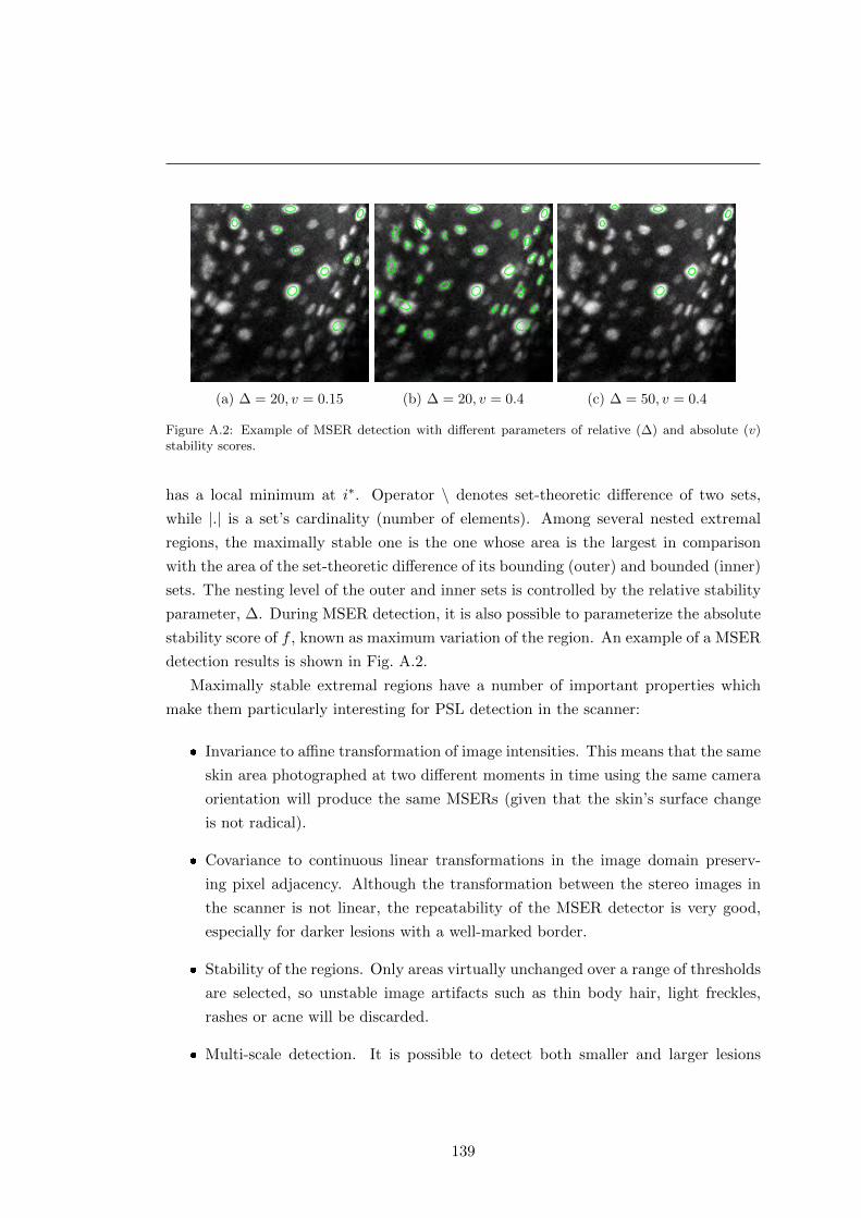
(a) ∆ = 20, v = 0.15 (b) ∆ = 20, v = 0.4 (c) ∆ = 50, v = 0.4
Figure A.2: Example of MSER detection with different parameters of relative (∆) and absolute (v)stability scores.
has a local minimum at i∗. Operator \ denotes set-theoretic difference of two sets,
while |.| is a set’s cardinality (number of elements). Among several nested extremal
regions, the maximally stable one is the one whose area is the largest in comparison
with the area of the set-theoretic difference of its bounding (outer) and bounded (inner)
sets. The nesting level of the outer and inner sets is controlled by the relative stability
parameter, ∆. During MSER detection, it is also possible to parameterize the absolute
stability score of f , known as maximum variation of the region. An example of a MSER
detection results is shown in Fig. A.2.
Maximally stable extremal regions have a number of important properties which
make them particularly interesting for PSL detection in the scanner:
� Invariance to affine transformation of image intensities. This means that the same
skin area photographed at two different moments in time using the same camera
orientation will produce the same MSERs (given that the skin’s surface change
is not radical).
� Covariance to continuous linear transformations in the image domain preserv-
ing pixel adjacency. Although the transformation between the stereo images in
the scanner is not linear, the repeatability of the MSER detector is very good,
especially for darker lesions with a well-marked border.
� Stability of the regions. Only areas virtually unchanged over a range of thresholds
are selected, so unstable image artifacts such as thin body hair, light freckles,
rashes or acne will be discarded.
� Multi-scale detection. It is possible to detect both smaller and larger lesions
139

A. METHODOLOGY
without specific multi-scale processing.
� Fast detection: the set of all extremal regions can be enumerated in O(n log log n).
The algorithm’s performance is very important given the amount of images to be
processed per exploration. The processing speed can be additionally improved by
detecting MSERs in resized images.
In this project, we used the Matlab® implementation of the MSER algorithm from
the VLFeat library [402].
A.2 Epipolar geometry
Epipolar geometry is the intrinsic projective geometry between two views of a scene [388].
It is defined by the intersection of the image planes with the family of planes passing
through the line joining the camera centers (the baseline). Fig. A.3 describes the epipo-
lar geometry in the context of a point correspondence search. A point X in space is
viewed at x and x′ by the cameras with centers C and C′, respectively. The baseline
of the cameras is the segment CC′. The epiploar geometry in a generic camera view
configuration, such as the one in Fig. A.3, is defined by the following elements:
� The epipoles e and e′. These are the points of intersection of the baseline with
the camera planes. Equivalently, e is the image of C′ in the left view, and e′ is
the image of C in the right view.
� An epipolar plane passing through the baseline CC′. As shown in Fig. A.3, this
plane also passes through the point in space X, and its projections x and x′.
� Epipolar lines produced by the intersection of an epipolar plane with the image
planes (in Fig. A.3, these are l and l′). All epipolar lines intersect at the epipole.
Thus, knowing the coordinates of one of the projections, x, the coordinates of the other
projection, x′, can be found along line l′. In other words, there is a projective mapping
x 7→ l′,
so that a point in one image corresponds to an epipolar line in the other image. This
mapping is defined by the so called fundamental matrix, F.
The definition of F can be derived using the notion of planar homography. Consid-
ering that the point in space X lies on plane π that does not pass through either of
140

Figure A.3: Point correspondence and epipolar geometry. The two cameras are represented by theirimage planes and centers C and C′. The line connecting the camera centers is called the baseline. Thebaseline intersects the image planes at points e and e′, called epipoles, which, together with the pointin space X, its projections x and x′, and the camera centers, lie on the epipolar plane. The intersectionof the epipolar plane with the image planes produces epipolar lines, l and l′. If X lies on plane π thatdoes not pass through either of the two camera centers, projections x and x′ are related by a planarhomography Hπ: x′ = Hπx.
the two camera centers (Fig. A.3), the projections x and x′ will be related by a planar
homography, Hπ:
x′ = Hπx.
Furthermore, the epipolar line l′ passing through x′ and the epipole e′ can be defined
as a cross-product:
l′ = e′ × x′ =
0 −e3 e2
e3 0 −e1
−e2 e1 0
x′1
x′2x′3
= [e′]×x′.
Since x′ = Hπx, we have
l′ = [e′]×Hπx = Fx,
where F = [e′]×Hπ is the fundamental matrix. It is a rank 2 homogreneous matrix with
7 degrees of freedom. For the corresponding image points x and x′, x′TFx = 0, while
for the epipoles: Fe = 0 and FTe′ = 0.
For a stereo rig, calibrated both intrinsically and extrinsically, the fundamental
matrix can be computed from the essential matrix. The essential matrix is the spe-
cialization of the fundamental matrix to the case of the normalized image coordinates:
141
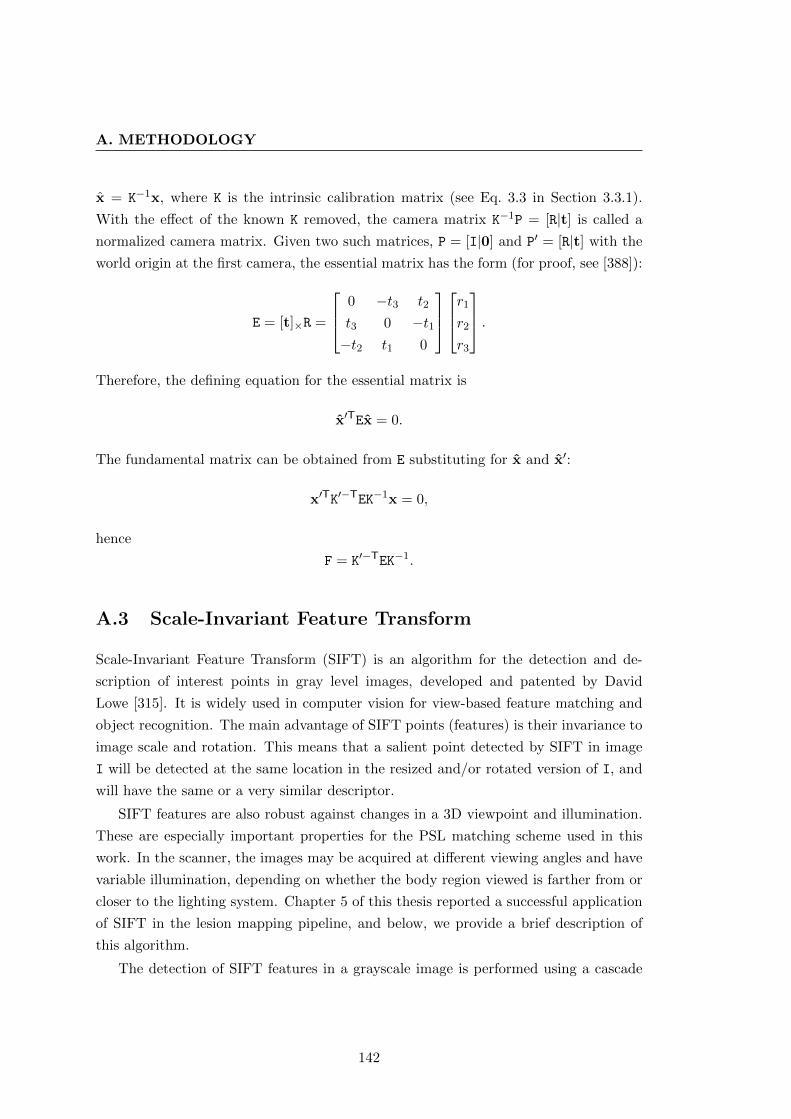
A. METHODOLOGY
x = K−1x, where K is the intrinsic calibration matrix (see Eq. 3.3 in Section 3.3.1).
With the effect of the known K removed, the camera matrix K−1P = [R|t] is called a
normalized camera matrix. Given two such matrices, P = [I|0] and P′ = [R|t] with the
world origin at the first camera, the essential matrix has the form (for proof, see [388]):
E = [t]×R =
0 −t3 t2
t3 0 −t1−t2 t1 0
r1
r2
r3
.Therefore, the defining equation for the essential matrix is
x′TEx = 0.
The fundamental matrix can be obtained from E substituting for x and x′:
x′TK′−TEK−1x = 0,
hence
F = K′−TEK−1.
A.3 Scale-Invariant Feature Transform
Scale-Invariant Feature Transform (SIFT) is an algorithm for the detection and de-
scription of interest points in gray level images, developed and patented by David
Lowe [315]. It is widely used in computer vision for view-based feature matching and
object recognition. The main advantage of SIFT points (features) is their invariance to
image scale and rotation. This means that a salient point detected by SIFT in image
I will be detected at the same location in the resized and/or rotated version of I, and
will have the same or a very similar descriptor.
SIFT features are also robust against changes in a 3D viewpoint and illumination.
These are especially important properties for the PSL matching scheme used in this
work. In the scanner, the images may be acquired at different viewing angles and have
variable illumination, depending on whether the body region viewed is farther from or
closer to the lighting system. Chapter 5 of this thesis reported a successful application
of SIFT in the lesion mapping pipeline, and below, we provide a brief description of
this algorithm.
The detection of SIFT features in a grayscale image is performed using a cascade
142
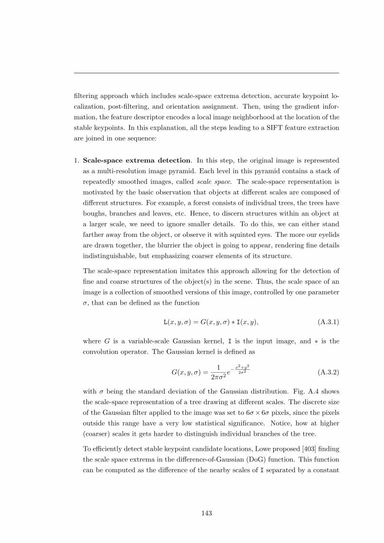
filtering approach which includes scale-space extrema detection, accurate keypoint lo-
calization, post-filtering, and orientation assignment. Then, using the gradient infor-
mation, the feature descriptor encodes a local image neighborhood at the location of the
stable keypoints. In this explanation, all the steps leading to a SIFT feature extraction
are joined in one sequence:
1. Scale-space extrema detection. In this step, the original image is represented
as a multi-resolution image pyramid. Each level in this pyramid contains a stack of
repeatedly smoothed images, called scale space. The scale-space representation is
motivated by the basic observation that objects at different scales are composed of
different structures. For example, a forest consists of individual trees, the trees have
boughs, branches and leaves, etc. Hence, to discern structures within an object at
a larger scale, we need to ignore smaller details. To do this, we can either stand
farther away from the object, or observe it with squinted eyes. The more our eyelids
are drawn together, the blurrier the object is going to appear, rendering fine details
indistinguishable, but emphasizing coarser elements of its structure.
The scale-space representation imitates this approach allowing for the detection of
fine and coarse structures of the object(s) in the scene. Thus, the scale space of an
image is a collection of smoothed versions of this image, controlled by one parameter
σ, that can be defined as the function
L(x, y, σ) = G(x, y, σ) ∗ I(x, y), (A.3.1)
where G is a variable-scale Gaussian kernel, I is the input image, and ∗ is the
convolution operator. The Gaussian kernel is defined as
G(x, y, σ) =1
2πσ2e−
x2+y2
2σ2 (A.3.2)
with σ being the standard deviation of the Gaussian distribution. Fig. A.4 shows
the scale-space representation of a tree drawing at different scales. The discrete size
of the Gaussian filter applied to the image was set to 6σ×6σ pixels, since the pixels
outside this range have a very low statistical significance. Notice, how at higher
(coarser) scales it gets harder to distinguish individual branches of the tree.
To efficiently detect stable keypoint candidate locations, Lowe proposed [403] finding
the scale space extrema in the difference-of-Gaussian (DoG) function. This function
can be computed as the difference of the nearby scales of I separated by a constant
143
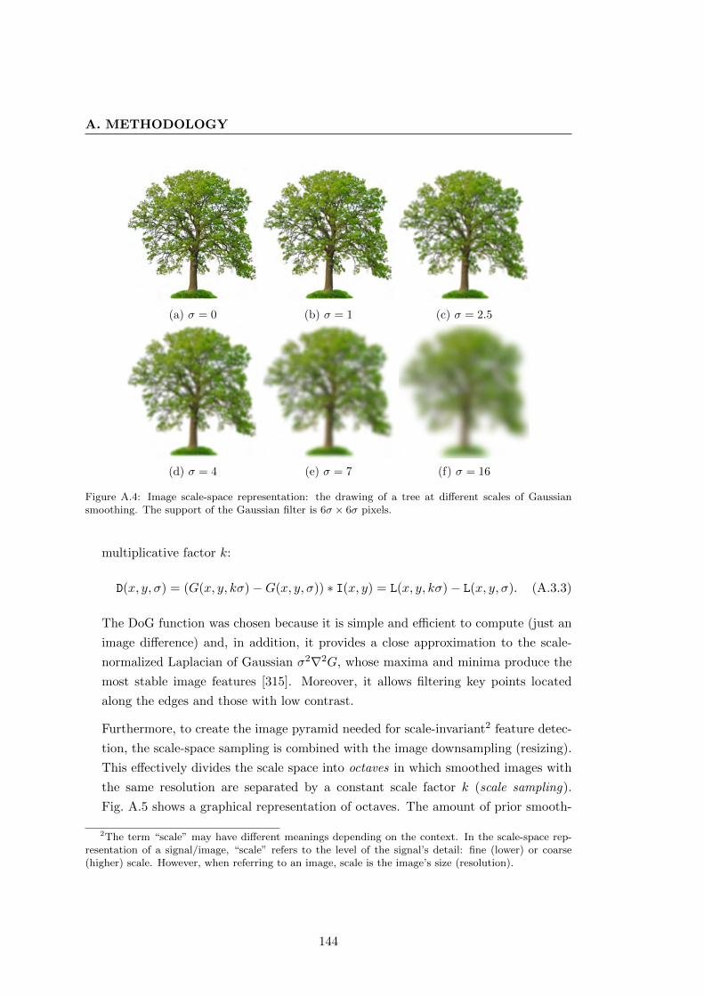
A. METHODOLOGY
(a) σ = 0 (b) σ = 1 (c) σ = 2.5
(d) σ = 4 (e) σ = 7 (f) σ = 16
Figure A.4: Image scale-space representation: the drawing of a tree at different scales of Gaussiansmoothing. The support of the Gaussian filter is 6σ × 6σ pixels.
multiplicative factor k:
D(x, y, σ) = (G(x, y, kσ)−G(x, y, σ)) ∗ I(x, y) = L(x, y, kσ)− L(x, y, σ). (A.3.3)
The DoG function was chosen because it is simple and efficient to compute (just an
image difference) and, in addition, it provides a close approximation to the scale-
normalized Laplacian of Gaussian σ2∇2G, whose maxima and minima produce the
most stable image features [315]. Moreover, it allows filtering key points located
along the edges and those with low contrast.
Furthermore, to create the image pyramid needed for scale-invariant2 feature detec-
tion, the scale-space sampling is combined with the image downsampling (resizing).
This effectively divides the scale space into octaves in which smoothed images with
the same resolution are separated by a constant scale factor k (scale sampling).
Fig. A.5 shows a graphical representation of octaves. The amount of prior smooth-
2The term “scale” may have different meanings depending on the context. In the scale-space rep-resentation of a signal/image, “scale” refers to the level of the signal’s detail: fine (lower) or coarse(higher) scale. However, when referring to an image, scale is the image’s size (resolution).
144
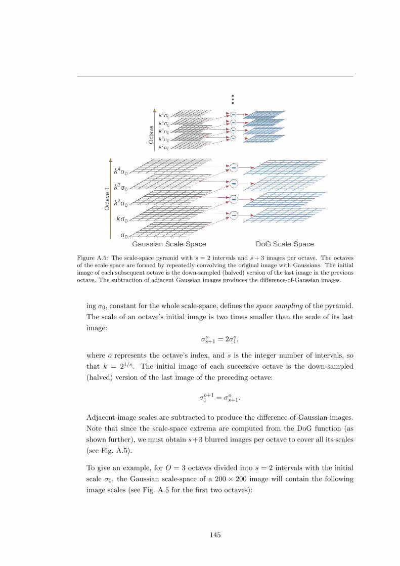
Figure A.5: The scale-space pyramid with s = 2 intervals and s + 3 images per octave. The octavesof the scale space are formed by repeatedly convolving the original image with Gaussians. The initialimage of each subsequent octave is the down-sampled (halved) version of the last image in the previousoctave. The subtraction of adjacent Gaussian images produces the difference-of-Gaussian images.
ing σ0, constant for the whole scale-space, defines the space sampling of the pyramid.
The scale of an octave’s initial image is two times smaller than the scale of its last
image:
σos+1 = 2σo1,
where o represents the octave’s index, and s is the integer number of intervals, so
that k = 21/s. The initial image of each successive octave is the down-sampled
(halved) version of the last image of the preceding octave:
σo+11 = σos+1.
Adjacent image scales are subtracted to produce the difference-of-Gaussian images.
Note that since the scale-space extrema are computed from the DoG function (as
shown further), we must obtain s+3 blurred images per octave to cover all its scales
(see Fig. A.5).
To give an example, for O = 3 octaves divided into s = 2 intervals with the initial
scale σ0, the Gaussian scale-space of a 200 × 200 image will contain the following
image scales (see Fig. A.5 for the first two octaves):
145

A. METHODOLOGY
Figure A.6: Extrema detection in the difference-of-Gaussian images. The pixel of interest in a DoGimage is compared to its 26 neighbors in the 3× 3 region at the current and adjacent scales (above andbelow). A pixel is considered an extremum if it is larger or smaller than all of the 26 neighbors. Pixelsbelonging to the scales at the top and bottom of a DoG octave are not checked for extrema.
Octave 1 (200× 200): σ0 212σ0 2σ0 2
32σ0 4σ0
Octave 2 (100× 100): 2σ0 232σ0 4σ0 2
52σ0 8σ0
Octave 3 (50× 50): 4σ0 252σ0 8σ0 2
72σ0 16σ0
2. Keypoint localization. To detect local extrema in the DoG images, each sample
point (pixel) is compared to its 26 neighbors: 8 at the same image scale and 9 at the
scales immediately above and below (see Fig. A.6). The point will be selected only if
it is larger or smaller than all of its neighbors. The experiments conducted by Lowe
in [315] showed that the highest repeatability of keypoint detection with respect to
location and scale was achieved with prior smoothing σ0 = 1.6 and s = 3 intervals
per octave. Moreover, if the original image is doubled in size after smoothing with
σ = 0.5, it increases the number of stable keypoints by a factor of almost 4.
Once the local extrema in the DoG images have been found, their locations are
refined by using quadratic interpolation. For that purpose, the author used the
Taylor expansion up to the quadratic terms to represent the DoG image:
D(x0 + h) = D(x0) +
(∂D
∂x
)T ∣∣∣∣x=x0
· h +1
2hT · ∂
2D
∂x2
∣∣∣∣x=x0
· h, (A.3.4)
where x0 is the candidate extremum point, h = (x, y, σ)T is the offset from x0 to
the precise location of the extremum, and
∂D
∂x=
∂D∂x∂D∂y∂D∂σ
and∂2D
∂x2=
Dxx Dxy Dxσ
Dyx Dyy Dyσ
Dσx Dσy Dσσ
are the first- and the second-order derivatives (Hessian matrix) of D at the candidate
146

point. The offset h to the precise extremum point is found by taking the derivative
of D (Eq. A.3.4) with respect to h and setting it at zero:
∂D
∂x
∣∣∣∣x=x0
+∂2D
∂x2
∣∣∣∣x=x0
· h = 0.
Hence,
h = −
(∂2D
∂x2
∣∣∣∣x=x0
)−1
· ∂D∂x
∣∣∣∣x=x0
. (A.3.5)
The derivative and the Hessian are approximated by neighboring pixel differences,
and the resulting 3×3 linear system of equations can be solved with minimal cost. If
the offset value h is larger than 0.5 in any dimension, it means that the extremum lies
closer to a different sample point, and the interpolation is performed there instead.
3. Keypoint filtering. The unstable extrema points (keypoints with low contrast) are
rejected by thresholding the value of D at the interpolated location h. The authors
chose to discard all extrema with |D(h)|< 0.03 corresponding to the “peak threshold”.
The value of |D(h)| can be found by substituting equation A.3.5 into A.3.4:
D(h) = D(x0) +1
2
(∂D
∂x
)T ∣∣∣∣x=x0
· h. (A.3.6)
Keypoints originating from edges are often represented by flat peaks in the DoG
function, which makes them unstable in the presence of noise. These keypoints can
be removed by evaluating the principal curvatures3 of D at the corresponding peak.
The idea is that a poorly defined peak will have a large principal curvature across
the edge, but a small one in the perpendicular direction. Therefore, we can discard
peaks based on the ratio of the principal curvatures only.
This ratio can be obtained from Hessian matrix H computed at the location and
the scale of keypoint x:
H(x) =
[Dxx Dxy
Dxy Dyy
]. (A.3.7)
The eigenvalues of Hessian matrix H(x) are proportional to the principal curvatures
of D(x), but their explicit computation can be avoided by finding the trace and the
3The principal curvatures are the maximum and minimum normal curvatures of a regular surface ata given point. The normal curvature at a point is the amount of the curve’s curvature in the directionof the surface normal.
147

A. METHODOLOGY
determinant of H(x), respectively:
Tr(H(x)) = Dxx + Dyy = e1 + e2,
Det(H(x)) = DxxDyy − (Dxy)2 = e1e2.
Here, e1 is the eigenvalue with the largest magnitude and e2 is the smallest one.
By representing the ratio between the eigenvalues as e1 = r · e2, we can obtain an
equation with only one unknown, r:
Tr(H(x))2
Det(H(x))=
(e1 + e2)2
e1e2=
(re2 + e2)2
re22
=(r + 1)2
r. (A.3.8)
Thus, to discard keypoints with a principal curvature ratio below some threshold,
r, it is enough to check that
Tr(H(x))2
Det(H(x))<
(r + 1)2
r.
The experiments conducted in [315] assumed an “edge threshold” r = 10.
4. Keypoint orientation assignment. The filtered keypoints can be invariant to ro-
tation if they are represented relative to their orientation in the local neighborhood.
This representation is done by means of a histogram of gradient orientations. In par-
ticular, using the scale of the keypoint of interest, we select the Gaussian smoothed
image L with the closest scale, σL. For each pixel in L, the graident magnitude
m(x, y) and orientation θ(x, y) are precomputed using the pixel differences:
m(x, y) =√
(L(x+ 1, y)− L(x− 1, y))2 + (L(x, y + 1)− L(x, y − 1))2,
θ(x, y) = tan−1L(x, y + 1)− L(x, y − 1)
L(x+ 1, y)− L(x− 1, y).
An orientation histogram is formed within a region around the keypoint of interest
defined by a Gaussian-weighted circular window, GL with a standard deviation 1.5 ·σL. This histogram consists of 36 bins covering a 360° range of orientations. The
pixels added to the histogram are weighted by their gradient magnitude and GL.
Peaks of this orientation histogram correspond to dominant directions of the gradi-
ents in the neighborhood. The keypoint is assigned the orientation corresponding
to the highest peak, as well as any other peak within 80% of the highest magnitude
(up to 2 peaks in total). In this way, there can be several keypoints with the same
148
Figure A.7: Creation of a SIFT keypoint descriptor. First, the gradient magnitude and orientationare computed at each image sample point in a region around the keypoint location and weighted bya Gaussian window (blue circle). The computed samples are then accumulated into a 2 × 2 array oforientation histograms that summarize the contents over 4 × 4 neighborhoods (shown on the right).Each histogram consists of 8 bins, and the lengths of the arrows correspond to the sum of gradientmagnitudes of all samples falling into that bin. In the experiments described in [315], the author used4× 4 descriptors computed from 16× 16 sample regions.
location and scale but different orientations. This approach contributes significantly
to the stability of feature matching.
5. Local image description. The keypoints acquired using the previous operations
have an assigned image location, scale and orientation. In this step, SIFT creates a
distinct encoding of the local image information around the points which makes the
features robust against changes in 3D viewpoint and illumination. At first, orienta-
tions and magnitudes of the image gradient are sampled around the feature location
in the blurred image of the Gaussian scale-space corresponding to the scale of the
feature.4 In order to achieve orientation invariance, the coordinates of the descriptor
and the gradient orientations are rotated relative to the keypoint’s orientation. In
Fig. A.7 (left), the gradients are denoted by small arrows: the longer the arrow, the
larger the magnitude of the gradient. The magnitude of each gradient is weighted
by means of a Gaussian function with σd = 12wd, where wd is the width of the
descriptor. The weighting window is centered on the descriptor as shown by the
blue transparent circle in Fig. A.7. This window is used to avoid abrupt changes
in the descriptor due to small shifts in the keypoint’s location. In addition, it gives
less importance to pixels farther from the center of the descriptor which are more
susceptible to misregistration errors.
4The gradients were precomputed for all levels in the pyramid in the previous step.
149
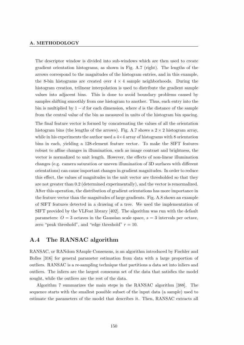
A. METHODOLOGY
The descriptor window is divided into sub-windows which are then used to create
gradient orientation histograms, as shown in Fig. A.7 (right). The lengths of the
arrows correspond to the magnitudes of the histogram entries, and in this example,
the 8-bin histograms are created over 4 × 4 sample neighborhoods. During the
histogram creation, trilinear interpolation is used to distribute the gradient sample
values into adjacent bins. This is done to avoid boundary problems caused by
samples shifting smoothly from one histogram to another. Thus, each entry into the
bin is multiplied by 1− d for each dimension, where d is the distance of the sample
from the central value of the bin as measured in units of the histogram bin spacing.
The final feature vector is formed by concatenating the values of all the orientation
histogram bins (the lengths of the arrows). Fig. A.7 shows a 2× 2 histogram array,
while in his experiments the author used a 4×4 array of histograms with 8 orientation
bins in each, yielding a 128-element feature vector. To make the SIFT features
robust to affine changes in illumination, such as image contrast and brightness, the
vector is normalized to unit length. However, the effects of non-linear illumination
changes (e.g. camera saturation or uneven illumination of 3D surfaces with different
orientations) can cause important changes in gradient magnitudes. In order to reduce
this effect, the values of magnitudes in the unit vector are thresholded so that they
are not greater than 0.2 (determined experimentally), and the vector is renormalized.
After this operation, the distribution of gradient orientations has more importance in
the feature vector than the magnitudes of large gradients. Fig. A.8 shows an example
of SIFT features detected in a drawing of a tree. We used the implementation of
SIFT provided by the VLFeat library [402]. The algorithm was run with the default
parameters: O = 3 octaves in the Gaussian scale space, s = 3 intervals per octave,
zero “peak threshold”, and “edge threshold” r = 10.
A.4 The RANSAC algorithm
RANSAC, or RANdom SAmple Consensus, is an algorithm introduced by Fischler and
Bolles [316] for general parameter estimation from data with a large proportion of
outliers. RANSAC is a re-sampling technique that partitions a data set into inliers and
outliers. The inliers are the largest consensus set of the data that satisfies the model
sought, while the outliers are the rest of the data.
Algorithm 7 summarizes the main steps in the RANSAC algorithm [388]. The
sequence starts with the smallest possible subset of the input data (a sample) used to
estimate the parameters of the model that describes it. Then, RANSAC extracts all
150
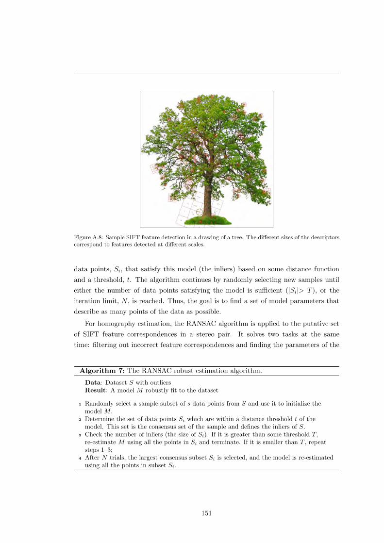
Figure A.8: Sample SIFT feature detection in a drawing of a tree. The different sizes of the descriptorscorrespond to features detected at different scales.
data points, Si, that satisfy this model (the inliers) based on some distance function
and a threshold, t. The algorithm continues by randomly selecting new samples until
either the number of data points satisfying the model is sufficient (|Si|> T ), or the
iteration limit, N , is reached. Thus, the goal is to find a set of model parameters that
describe as many points of the data as possible.
For homography estimation, the RANSAC algorithm is applied to the putative set
of SIFT feature correspondences in a stereo pair. It solves two tasks at the same
time: filtering out incorrect feature correspondences and finding the parameters of the
Algorithm 7: The RANSAC robust estimation algorithm.
Data: Dataset S with outliersResult: A model M robustly fit to the dataset
1 Randomly select a sample subset of s data points from S and use it to initialize themodel M .
2 Determine the set of data points Si which are within a distance threshold t of themodel. This set is the consensus set of the sample and defines the inliers of S.
3 Check the number of inliers (the size of Si). If it is greater than some threshold T ,re-estimate M using all the points in Si and terminate. If it is smaller than T , repeatsteps 1–3;
4 After N trials, the largest consensus subset Si is selected, and the model is re-estimatedusing all the points in subset Si.
151

A. METHODOLOGY
Algorithm 8: Adaptive algorithm for determining the number of RANSAC sam-ples, N .
Data: Dataset S
1 N =∞ ; /* Number of samples */
2 n = 0 ; /* Sample count */
3 while N > n do4 Choose a sample of s points and count the number of inliers, |Si|;5 ε = 1− |Si|/|S| ; /* Probability that a data point is an outlier */
6 Compute N for p = 0.99 (Eq.A.4.2);7 n = n+ 1;
8 end
homography matrix between the two images. Each sample used by RANSAC for this
purpose is size s = 4, and the distance function is defined as the symmetric transfer
error:
d2transfer = d(x, H−1x′)2 + d(x′, Hx)2, (A.4.1)
where x ↔ x′ are the point correspondences in the two images, H is the estimated
homography, and d returns the Euclidean distance between the points.
One of the key features of the RANSAC approach is that, instead of trying every
possible sample for model estimation, it uses a limited number of randomly selected
samples, N . This number is chosen high enough to ensure a probability (normally,
p = 0.99) that at least one of the random samples of s points does not contain any
outliers. If ι is the probability that any selected point is an inlier, ε = 1− ι defines the
probability that it is an outlier. Thus, we need to select at least N samples, containing
s points each, in order to obtain one that is free of outliers with a probability p:
(1− ιs)N = 1− p,
hence,
N =log(1− p)
log(1− (1− ε)s). (A.4.2)
When ε is unknown, the number of samples can be set adaptively as the proportion of
outliers determined from each consensus set, as described in Algorithm 8.
In our pipeline, we used the implementation of RANSAC for homography computa-
tion from [404], which does not employ the T threshold and relies only on the adaptive
N . The value of the distance threshold, t, was set to 0.05.
152
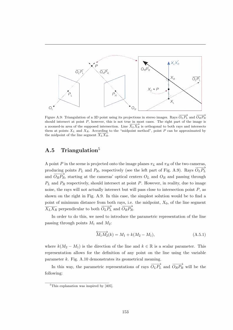
Figure A.9: Triangulation of a 3D point using its projections in stereo images. Rays−−−→OLPL and
−−−→ORPR
should intersect at point P , however, this is not true in most cases. The right part of the image is
a zoomed-in area of the supposed intersection. Line−−−−→XLXR is orthogonal to both rays and intersects
them at points XL and XR. According to the “midpoint method”, point P can be approximated bythe midpoint of the line segment XLXR.
A.5 Triangulation5
A point P in the scene is projected onto the image planes πL and πR of the two cameras,
producing points PL and PR, respectively (see the left part of Fig. A.9). Rays−−−→OLPL
and−−−→ORPR, starting at the cameras’ optical centers OL and OR and passing through
PL and PR respectively, should intersect at point P . However, in reality, due to image
noise, the rays will not actually intersect but will pass close to intersection point P , as
shown on the right in Fig. A.9. In this case, the simplest solution would be to find a
point of minimum distance from both rays, i.e. the midpoint, X0, of the line segment
XLXR perpendicular to both−−−→OLPL and
−−−→ORPR.
In order to do this, we need to introduce the parametric representation of the line
passing through points M1 and M2:
←−−→M1M2(k) = M1 + k(M2 −M1), (A.5.1)
where k(M2 −M1) is the direction of the line and k ∈ R is a scalar parameter. This
representation allows for the definition of any point on the line using the variable
parameter k. Fig. A.10 demonstrates its geometrical meaning.
In this way, the parametric representations of rays−−−→OLPL and
−−−→ORPR will be the
following:
5This explanation was inspired by [405].
153
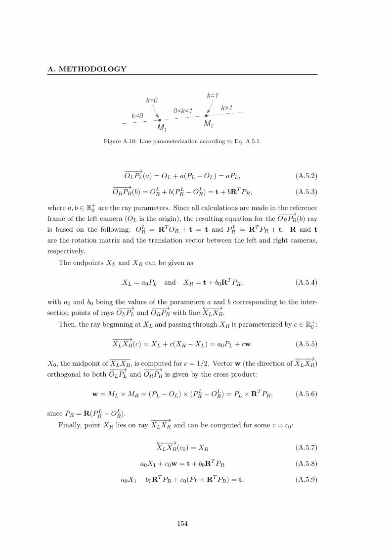
A. METHODOLOGY
Figure A.10: Line parameterization according to Eq. A.5.1.
−−−→OLPL(a) = OL + a(PL −OL) = aPL, (A.5.2)
−−−→ORPR(b) = OLR + b(PLR −OLR) = t + bRTPR, (A.5.3)
where a, b ∈ R+0 are the ray parameters. Since all calculations are made in the reference
frame of the left camera (OL is the origin), the resulting equation for the−−−→ORPR(b) ray
is based on the following: OLR = RTOR + t = t and PLR = RTPR + t. R and t
are the rotation matrix and the translation vector between the left and right cameras,
respectively.
The endpoints XL and XR can be given as
XL = a0PL and XR = t + b0RTPR, (A.5.4)
with a0 and b0 being the values of the parameters a and b corresponding to the inter-
section points of rays−−−→OLPL and
−−−→ORPR with line
←−−→XLXR.
Then, the ray beginning at XL and passing through XR is parameterized by c ∈ R+0 :
−−−−→XLXR(c) = XL + c(XR −XL) = a0PL + cw. (A.5.5)
X0, the midpoint of XLXR, is computed for c = 1/2. Vector w (the direction of−−−−→XLXR)
orthogonal to both−−−→OLPL and
−−−→ORPR is given by the cross-product:
w = ML ×MR = (PL −OL)× (PLR −OLR) = PL ×RTPR, (A.5.6)
since PR = R(PLR −OLR).
Finally, point XR lies on ray−−−−→XLXR and can be computed for some c = c0:
←−−→XLXR(c0) = XR (A.5.7)
a0X1 + c0w = t + b0RTPR (A.5.8)
a0X1 − b0RTPR + c0(PL ×RTPR) = t. (A.5.9)
154

After solving the system of equations A.5.9 for a0, b0 and c0, points XL and XR can
be easily found from equation A.5.4. With the points obtained, X0 can be computed
from the parameterized equation A.5.5 for−−−−→XLXR.
155

A. METHODOLOGY
156

References
[1] H. Kaufman, The melanoma book: a complete guide to prevention and treatment, 1st ed.
New York: Gotham Books, 2005. 2, 3, 5
[2] S. Cade, “Malignant melanoma: Bradshaw Lecture delivered at the Royal College of
Surgeons of England on 7th December 1960,” Ann. R. Coll. Surg. Engl., vol. 28, pp.
331–6, 1961. 1, 17, 45, 71
[3] J. A. McGrath and J. Uitto, “Anatomy and organization of human skin,” in Rook’s
Textbook of Dermatology, T. Burns, S. Breathnach, N. Cox, and C. Griffiths, Eds.
Oxford: Wiley-Blackwell, 2010, ch. 3, pp. 1–53. 2, 3
[4] A. Jerant, J. Johnson, C. Sheridan, and T. Caffrey, “Early detection and treatment of
skin cancer,” Am. Fam. Physician, vol. 62, no. 2, pp. 357–386, 2000. 3, 6
[5] J. Newton Bishop, “Lentigos, melanocytic naevi and melanoma,” in Rook’s Textbook of
Dermatology, T. Burns, S. Breathnach, N. Cox, and C. Griffiths, Eds. Oxford: Wiley-
Blackwell, 2010, ch. 54, pp. 1–57. 5, 6
[6] R. Friedman, D. Rigel, and A. Kopf, “Early detection of malignant melanoma: The role
of physician examination and self-examination of the skin,” CA-Cancer J. Clin., vol. 35,
no. 3, pp. 130–151, 1985. 5, 7, 11
[7] W. Norris, “Case of fungoid disease,” Edinburgh Medical and Surgical Journal, vol. 16,
pp. 562–5, 1820. 5
[8] J. P. Bennett and P. Hall, “Moles and melanoma: a history,” Ann. R. Coll. Surg. Engl.,
vol. 76, no. 6, p. 373, 1994. 5, 131
[9] S. Markovic, L. Erickson, R. Rao, R. McWilliams, L. Kottschade, E. Creagan et al.,
“Malignant melanoma in the 21st century, part 1: epidemiology, risk factors, screening,
prevention, and diagnosis,” Mayo Clin. Proc., vol. 82, no. 3, pp. 364–380, 2007. 6, 7
[10] American Cancer Society, “Cancer facts & figures 2013,” Atlanta: American Cancer
Society, Tech. Rep., 2013. 6, 14
[11] A. Breslow, “Thickness, cross-sectional areas and depth of invasion in the prognosis of
cutaneous melanoma.” Ann. Surg., vol. 172, no. 5, p. 902, 1970. 6, 7
157
REFERENCES
[12] A. Marghoob, L. Swindle, C. Moricz, F. Sanchez Negron, B. Slue, A. Halpern, and
A. Kopf, “Instruments and new technologies for the in vivo diagnosis of melanoma,” J.
Am. Acad. Dermatol., vol. 49, no. 5, pp. 777–797, 2003. 7
[13] A. Halpern, “Total body skin imaging as an aid to melanoma detection,” Semin. Cutan.
Med. Surg., vol. 22, no. 1, pp. 2–8, 2003. 7, 8, 9, 43
[14] D. Ratner, C. Thomas, and D. Bickers, “The uses of digital photography in dermatology,”
J. Am. Acad. Dermatol., vol. 41, no. 5, pp. 749–756, 1999. 7
[15] J. Quintana, “Computer vision techniques for early detection of skin cancer,” Ph.D.
dissertation, University of Girona, 2012. 7, 132
[16] L. Smith and S. MacNeil, “State of the art in non-invasive imaging of cutaneous
melanoma,” Skin Res. Tech., vol. 17, no. 3, pp. 257–269, 2011. 7
[17] D. Rigel, J. Russak, and R. Friedman, “The evolution of melanoma diagnosis: 25 years
beyond the ABCDs,” CA-Cancer J. Clin., vol. 60, no. 5, pp. 301–316, 2010. 7, 11
[18] S. Wang and P. Hashemi, “Noninvasive imaging technologies in the diagnosis of mela-
noma,” Semin. Cutan. Med. Surg., vol. 29, no. 3, pp. 174–184, 2010. 7
[19] A. Gadeliya Goodson and D. Grossman, “Strategies for early melanoma detection: Ap-
proaches to the patient with nevi,” J. Am. Acad. Dermatol., vol. 60, no. 5, pp. 719–735,
2009. 7
[20] E. Psaty and A. Halpern, “Current and emerging technologies in melanoma diagnosis:
the state of the art,” Clin. Dermatol., vol. 27, no. 1, pp. 35–45, 2009. 7
[21] A. Esmaeili, A. Scope, A. C. Halpern, and A. A. Marghoob, “Imaging techniques for
the in vivo diagnosis of melanoma,” Semin. Cutan. Med. Surg., vol. 27, no. 1, pp. 2–10,
2008. 7
[22] J. Patel, S. Konda, O. Perez, S. Amini, G. Elgart, and B. Berman, “Newer technolo-
gies/techniques and tools in the diagnosis of melanoma,” Eur. J. Dermatol., vol. 18,
no. 6, pp. 617–631, 2008. 7
[23] G. Day and R. Barbour, “Automated melanoma diagnosis: where are we at?” Skin Res.
Tech., vol. 6, no. 1, pp. 1–5, 2000. 8, 37
[24] A. Halpern, A. Marghoob, T. Bialoglow, W. Witmer, and W. Slue, “Standardized posi-
tioning of patients (poses) for whole body cutaneous photography,” J. Am. Acad. Der-
matol., vol. 49, no. 4, pp. 593–598, 2003. 8
[25] N. Feit, S. Dusza, and A. Marghoob, “Melanomas detected with the aid of total
cutaneous photography,” Br. J. Dermatol., vol. 150, no. 4, pp. 706–714, 2004. 8, 45
[26] M. Rademaker and A. Oakley, “Digital monitoring by whole body photography and
sequential digital dermoscopy detects thinner melanomas,” J. Prim. Health Care, vol. 2,
no. 4, pp. 267–272, 2010. 8
158
REFERENCES
[27] V. Terushkin, S. Oliveria, A. Marghoob, and A. Halpern, “Use of and beliefs about
total body photography and dermatoscopy among us dermatology training programs: An
update,” J. Am. Acad. Dermatol., vol. 62, no. 5, pp. 794–803, 2010. 9
[28] A. W. Kopf, M. Elbaum, and N. Provost, “The use of dermoscopy and digital imaging
in the diagnosis of cutaneous malignant melanoma,” Skin Res. Tech., vol. 3, no. 1, pp.
1–7, 1997. 9
[29] S. W. Menzies, “Automated epiluminescence microscopy: Human vs machine in the
diagnosis of melanoma,” Arch. Dermatol., vol. 135, no. 12, pp. 1538–40, 1999. 9
[30] G. Pellacani and S. Seidenari, “Comparison between morphological parameters in
pigmented skin lesion images acquired by means of epiluminescence surface microscopy
and polarized-light videomicroscopy,” Clin. Dermatol., vol. 20, no. 3, pp. 222–227, 2002.
9, 10, 50
[31] C. Benvenuto-Andrade, S. Dusza, A. Agero, M. Rajadhyaksha, A. Halpern, and
A. Marghoob, “Differences between polarized light dermoscopy and immersion contact
dermoscopy for the evaluation of skin lesions,” Arch. dermatol., vol. 143, no. 3, pp. 329–
338, 2007. 10
[32] S. Seidenari, G. Pellacani, and P. Pepe, “Digital videomicroscopy improves diagnostic
accuracy for melanoma,” J. Am. Acad. Dermatol., vol. 39, no. 2, pp. 175–181, 1998. 10,
36, 38
[33] X. Yuan, N. Situ, and G. Zouridakis, “A narrow band graph partitioning method for
skin lesion segmentation,” Pattern Recogn., vol. 42, no. 6, pp. 1017–28, 2009. 10, 23
[34] A. P. Dhawan, R. Gordon, and R. M. Rangayyan, “Nevoscopy: Three-dimensional com-
puted tomography of nevi and melanomas in situ by transillumination,” IEEE T. Med.
Imaging, vol. 3, no. 2, pp. 54–61, 1984. 10, 17, 40
[35] A. P. Dhawan, “Early detection of cutaneous malignant melanoma by three-dimensional
nevoscopy,” Comput. Meth. Programs Biomed., vol. 21, no. 1, pp. 59–68, 1985. 10, 40
[36] A. Dhawan, “Apparatus and method for skin lesion examination,” US Patent 5.146.923,
1992. 10
[37] J. Banky, J. Kelly, D. English, J. Yeatman, and J. Dowling, “Incidence of new and changed
nevi and melanomas detected using baseline images and dermoscopy in patients at high
risk for melanoma,” Arch. Dermatol., vol. 141, no. 8, pp. 998–1006, 2005. 10
[38] N. Abbasi, H. Shaw, D. Rigel, R. Friedman, W. McCarthy, I. Osman et al., “Early
diagnosis of cutaneous melanoma: Revisiting the ABCD criteria,” J. Am. Med. Assoc.,
vol. 292, no. 22, pp. 2771–76, 2004. 11, 30, 45
[39] R. Mackie and V. Doherty, “Seven-point checklist for melanoma,” Clin. Exp. Dermatol.,
vol. 16, no. 2, pp. 151–152, 1991. 11
159
REFERENCES
[40] H. Kittler, H. Pehamberger, K. Wolff, and M. Binder, “Follow-up of melanocytic skin
lesions with digital epiluminescence microscopy: Patterns of modifications observed in
early melanoma, atypical nevi, and common nevi,” J. Am. Acad. Dermatol., vol. 43,
no. 3, pp. 467–476, 2000. 11
[41] S. Menzies, A. Gutenev, M. Avramidis, A. Batrac, and W. McCarthy, “Short-term dig-
ital surface microscopic monitoring of atypical or changing melanocytic lesions,” Arch.
Dermatol., vol. 137, no. 12, pp. 1583–89, 2001. 11, 32, 35, 38
[42] J. Malvehy, S. Puig, G. Argenziano, A. A. Marghoob, and H. P. Soyer, “Dermoscopy
report: Proposal for standardization. Results of a consensus meeting of the International
Dermoscopy Society,” J. Am. Acad. Dermatol., vol. 57, no. 1, pp. 84–95, 2007. 11, 12,
27, 28, 30, 44
[43] G. Argenziano, H. Soyer, S. Chimenti, R. Talamini, R. Corona, F. Sera et al., “Der-
moscopy of pigmented skin lesions: Results of a consensus meeting via the Internet,” J.
Am. Acad. Dermatol., vol. 48, no. 5, pp. 679–693, 2003. 12
[44] G. Capdehourat, A. Corez, A. Bazzano, R. Alonso, and P. Muse, “Toward a combined
tool to assist dermatologists in melanoma detection from dermoscopic images of
pigmented skin lesions,” Pattern Recogn. Lett., vol. 32, no. 16, pp. 2187–2196, 2011. 12,
27, 36
[45] G. Day and R. Barbour, “Automated skin lesion screening—a new approach,” Melanoma
Res., vol. 11, no. 1, pp. 31–35, 2001. 12, 13, 14, 17, 22, 36
[46] R. Marchesini, A. Bono, C. Bartoli, M. Lualdi, S. Tomatis, and N. Cascinelli, “Optical
imaging and automated melanoma detection: questions and answers,” Melanoma Res.,
vol. 12, no. 3, pp. 279–286, 2002. 12, 37, 44
[47] M. Vestergaard and S. Menzies, “Automated diagnostic instruments for cutaneous mela-
noma,” Semin. Cutan. Med. Surg., vol. 27, no. 1, pp. 32–36, 2008. 12, 37, 39
[48] J. Fruhauf, B. Leinweber, R. Fink-Puches, V. Ahlgrimm-Siess, E. Richtig, I. Wolf et al.,
“Patient acceptance and diagnostic utility of automated digital image analysis of pig-
mented skin lesions,” J. Eur. Acad. Dermatol. Venereol., vol. 26, no. 3, pp. 368–372,
2011. 13, 44
[49] S. Dreiseitl and M. Binder, “Do physicians value decision support? A look at the effect
of decision support systems on physician opinion,” Artif. Intell. Med., vol. 33, no. 1, pp.
25–30, 2005. 14
[50] R. S. Stern, “Prevalence of a history of skin cancer in 2007: Results of an incidence-based
model,” Arch. Dermatol., vol. 146, no. 3, pp. 279–282, 2010. 14
[51] A. C. Halpern, “The use of whole body photography in a pigmented lesion clinic,”
Dermatol. Surg., vol. 26, no. 12, pp. 1175–80, 2000. 15
160
REFERENCES
[52] R. Drugge, C. Nguyen, L. Gliga, and E. Drugge, “Clinical pathway for melanoma detec-
tion using comprehensive cutaneous analysis with Melanoscan®,” Dermatol. Online J.,
vol. 16, no. 8, 2010. 15, 45
[53] W. V. Stoecker and R. H. Moss, “Editorial: digital imaging in dermatology,” Comput.
Med. Imaging Graph., vol. 16, no. 3, pp. 145–150, 1992. 17, 42
[54] A. Green, N. Martin, G. McKenzie, J. Pfitzner, F. Quintarelli, B. Thomas et al., “Com-
puter image analysis of pigmented skin lesions,” Melanoma Res., vol. 1, no. 4, pp. 231–236,
1991. 17, 30, 36
[55] M. E. Celebi, W. V. Stoecker, and R. H. Moss, “Advances in skin cancer image
analysis,” Comput. Med. Imaging Graph., vol. 35, no. 2, pp. 83–84, 2011. 17
[56] M. Celebi, H. Iyatomi, G. Schaefer, and W. Stoecker, “Lesion border detection in der-
moscopy images,” Comput. Med. Imaging Graph., vol. 33, no. 2, pp. 148–153, 2009. 17,
20, 22, 24, 25
[57] V. Berenguer, D. Ruiz, and A. Soriano, “Application of Hidden Markov Models to mel-
anoma diagnosis,” in Proc. Int. Symp. Distrib. Comput. and Artif. Intell., J. Corchado,
S. Rodriguez, J. Llinas, and J. Molina, Eds., vol. 50. Berlin: Springer, 2009, pp. 357–365.
19, 20, 21, 28, 33, 36
[58] S. Skrøvseth, T. Schopf, K. Thon, M. Zortea, M. Geilhufe, K. Mollersen et al., “A com-
puter aided diagnostic system for malignant melanomas,” in Proc. Int. Symp. Applied
Sciences in Biomed. and Comm. Tech. (ISABEL). Piscataway, NJ: IEEE Press, 2010,
pp. 1–5. 19, 27, 28, 33
[59] T. Lee, V. Ng, R. Gallagher, A. Coldman, and D. McLean, “DullRazor®: A software
approach to hair removal from images,” Comput. Biol. Med., vol. 27, no. 6, pp. 533–543,
1997. 20, 21
[60] M. G. Fleming, C. Steger, J. Zhang, J. Gao, A. B. Cognetta, llya Pollak, and C. R.
Dyer, “Techniques for a structural analysis of dermatoscopic imagery,” Comput. Med.
Imaging Graph., vol. 22, no. 5, pp. 375–389, 1998. 20, 21, 22, 23, 27
[61] O. Debeir, C. Decaestecker, J. Pasteels, I. Salmon, R. Kiss, and P. Van Ham, “Computer-
assisted analysis of epiluminescence microscopy images of pigmented skin lesions,” Cy-
tometry, vol. 37, no. 4, pp. 255–266, 1999. 20, 21, 23, 27
[62] D. H. Chung and G. Sapiro, “Segmenting skin lesions with partial-differential-equations-
based image processing algorithms,” IEEE T. Med. Imaging, vol. 19, no. 7, pp. 763–767,
2000. 20, 21, 23
[63] P. Schmid-Saugeon, J. Guillod, and J. Thiran, “Towards a computer-aided diagnosis
system for pigmented skin lesions,” Comput. Med. Imaging Graph., vol. 27, no. 1, pp.
65–78, 2003. 20, 21, 28
161
REFERENCES
[64] H. Zhou, M. Chen, R. Gass, J. Rehg, L. Ferris, J. Ho, and L. Drogowski, “Feature-
preserving artifact removal from dermoscopy images,” in Proc. SPIE, ser. Medical Imag-
ing: Image Processing, J. M. Reinhardt and J. P. W. Pluim, Eds., vol. 6914(1B). San
Diego, CA: SPIE, 2008. 20, 21
[65] P. Wighton, T. Lee, and M. Atkins, “Dermascopic hair disocclusion using inpainting,”
in Proc. SPIE, ser. Medical Imaging: Image Processing, J. M. Reinhardt and J. P. W.
Pluim, Eds., vol. 6914(27). San Diego, CA: SPIE, 2008. 20, 21
[66] F.-Y. Xie, S.-Y. Qin, Z.-G. Jiang, and R.-S. Meng, “PDE-based unsupervised repair of
hair-occluded information in dermoscopy images of melanoma,” Comput. Med. Imaging
Graph., vol. 33, no. 4, pp. 275–282, 2009. 20, 21
[67] C. Barcelos and V. Pires, “An automatic based nonlinear diffusion equations scheme for
skin lesion segmentation,” Appl. Math. Comput., vol. 215, no. 1, pp. 251–261, 2009. 20,
21, 23
[68] Q. Abbas, I. Fondon, and M. Rashid, “Unsupervised skin lesions border detection via
two-dimensional image analysis,” Comput. Meth. Programs Biomed., vol. 27, no. 1, pp.
65–78, 2010. 20, 21
[69] K. Møllersen, H. Kirchesch, T. Schopf, and F. Godtliebsen, “Unsupervised segmentation
for digital dermoscopic images,” Skin Res. Tech., vol. 16, no. 4, pp. 401–407, 2010. 20
[70] N. Nguyen, T. Lee, and M. Atkins, “Segmentation of light and dark hair in dermoscopic
images: a hybrid approach using a universal kernel,” in Proc. SPIE, ser. Medical Imaging:
Image Processing, B. M. Dawant and D. R. Haynor, Eds., vol. 7623(4N). San Diego,
CA: SPIE, 2010. 20, 21
[71] K. Kiani and A. R. Sharafat, “E-shaver: An improved DullRazor® for digitally removing
dark and light-colored hairs in dermoscopic images,” Comput. Biol. Med., vol. 41, no. 3,
pp. 139–145, 2011. 20, 21
[72] P. Wighton, T. Lee, H. Lui, D. McLean, and M. Atkins, “Generalizing common tasks in
automated skin lesion diagnosis,” IEEE T. Inf. Technol. B., vol. 4, pp. 622–629, 2011.
20, 21, 23, 27
[73] Q. Abbas, M. Celebi, and I. Garcia, “Hair removal methods: A comparative study for
dermoscopy images,” Biomed. Signal Process. Contr., vol. 6, no. 4, pp. 395–404, 2011.
20, 21
[74] Q. Abbas, M. E. Celebi, and I. F. Garcıa, “Skin tumor area extraction using an
improved dynamic programming approach,” Skin Res. Tech., vol. 18, no. 2, pp. 133–142,
2012. 20, 23
[75] A. Afonso and M. Silveira, “Hair detection in dermoscopic images using percolation,” in
Proc. IEEE Ann. Int. Conf. Eng. Med. Biol. Soc. (EMBC), 2012, pp. 4378–4381. 20
162
REFERENCES
[76] M. T. B. Toossi, H. R. Pourreza, H. Zare, M.-H. Sigari, P. Layegh, and A. Azimi, “An
effective hair removal algorithm for dermoscopy images,” Skin Res. Tech., vol. 19, pp.
230–235, 2013. 20
[77] A. Huang, S.-Y. Kwan, W.-Y. Chang, M.-Y. Liu, M.-H. Chi, and G.-S. Chen, “A robust
hair segmentation and removal approach for clinical images of skin lesions,” in Proc. IEEE
Ann. Int. Conf. Eng. Med. Biol. Soc. (EMBC), 2013, pp. 3315–3318. 20
[78] Q. Abbas, I. Garcıa, and M. Rashid, “Automatic skin tumour border detection for digital
dermoscopy using a new digital image analysis scheme,” Br. J. Biomed. Sci., vol. 67,
no. 4, pp. 177–183, 2010. 20, 21
[79] A. Gutenev, V. Skladnev, and D. Varvel, “Acquisition-time image quality control in
digital dermatoscopy of skin lesions,” Comput. Med. Imaging Graph., vol. 25, no. 6, pp.
495–499, 2001. 20
[80] E. Zagrouba and W. Barhoumi, “A preliminary approach for the automated recognition
of malignant melanoma,” Image Anal. Stereol., vol. 23, no. 2, pp. 121–135, 2004. 20, 21,
30, 36
[81] A. Chiem, A. Al-Jumaily, and R. Khushaba, “A novel hybrid system for skin lesion de-
tection,” in Proc. Int. Conf. Intell. Sensors, Sensor Netw. and Inform., M. Palaniswami,
S. Marusic, and Y. W. Law, Eds. Piscataway, NJ: IEEE Press, 2007, pp. 567–572. 20,
21, 28, 34, 36
[82] M. Messadi, A. Bessaid, and A. Taleb-Ahmed, “Extraction of specific parameters for skin
tumour classification,” J. Med. Eng. Tech., vol. 33, no. 4, pp. 288–295, 2009. 20, 28, 36
[83] M. E. Celebi, H. A. Kingravi, B. Uddin, H. Iyatomi, Y. A. Aslandogan, W. V. Stoecker,
and R. H. Moss, “A methodological approach to the classification of dermoscopy
images,” Comput. Med. Imaging Graph., vol. 31, no. 6, pp. 362–373, 2007. 20, 26, 28, 36
[84] A. Dhawan, B. D’Alessandro, S. Patwardhan, and N. Mullani, “Multispectral optical
imaging of skin-lesions for detection of malignant melanomas,” in Proc. IEEE Ann. Int.
Conf. Eng. Med. Biol. Soc. (EMBC). Piscataway, NJ: IEEE Press, 2009, pp. 5352–55.
20, 21
[85] D. Ruiz, V. Berenguer, A. Soriano, and B. Sanchez, “A decision support system for the
diagnosis of melanoma: A comparative approach,” Expert Syst. Appl., vol. 38, no. 12, pp.
15 217–23, 2011. 20, 21, 34, 36
[86] J. Blackledge and D. Dubovitskiy, “Object detection and classification with applications
to skin cancer screening,” ISAST T. Intelligent Systems, vol. 1, pp. 34–45, 2008. 20, 28,
29, 31, 36
[87] Y. Haeghen, J. Naeyaert, I. Lemahieu, and W. Philips, “An imaging system with cali-
brated color image acquisition for use in dermatology,” IEEE T. Med. Imaging, vol. 19,
no. 7, pp. 722–730, 2000. 20
163
REFERENCES
[88] C. Grana, G. Pellacani, and S. Seidenari, “Practical color calibration for dermoscopy,
applied to a digital epiluminescence microscope,” Skin Res. Tech., vol. 11, no. 4, pp.
242–247, 2005. 20
[89] H. Iyatomi, M. Celebi, G. Schaefer, and M. Tanaka, “Automated color calibration method
for dermoscopy images,” Comput. Med. Imaging Graph., vol. 35, no. 2, pp. 89–98, 2011.
20
[90] J. Quintana, R. Garcıa, and L. Neumann, “A novel method for color correction in
epiluminescence microscopy,” Comput. Med. Imaging Graph., vol. 35, no. 7-8, pp.
646–652, 2011. 20, 21
[91] P. Wighton, T. K. Lee, H. Lui, D. McLean, and M. S. Atkins, “Chromatic aberration
correction: an enhancement to the calibration of low-cost digital dermoscopes,” Skin
Res. Tech., vol. 17, no. 3, pp. 339–347, 2011. 20, 21
[92] J. Alcon, C. Ciuhu, W. ten Kate, A. Heinrich, N. Uzunbajakava, G. Krekels et al., “Au-
tomatic imaging system with decision support for inspection of pigmented skin lesions
and melanoma diagnosis,” IEEE J. Sel. Topics in Signal Proc., vol. 3, no. 1, pp. 14–25,
2009. 20, 30, 31, 36
[93] P. Cavalcanti and J. Scharcanski, “Automated prescreening of pigmented skin lesions
using standard cameras,” Comput. Med. Imaging Graph., vol. 35, pp. 481–491, 2011. 20,
26, 30, 36
[94] K.-A. Norton, H. Iyatomi, M. E. Celebi, S. Ishizaki, M. Sawada, R. Suzaki, K. Kobayashi
et al., “Three-phase general border detection method for dermoscopy images using
non-uniform illumination correction,” Skin Res. Tech., vol. 18, pp. 290–300, 2012. 20
[95] J. Glaister, R. Amelard, A. Wong, and D. Clausi, “Msim: Multistage illumination model-
ing of dermatological photographs for illumination-corrected skin lesion analysis,” IEEE
T. Biomed. Eng., vol. 60, no. 7, pp. 1873–83, July 2013. 20
[96] D. Delgado, C. Butakoff, B. Ersbøll, and W. Stoecker, “Independent histogram pursuit
for segmentation of skin lesions,” IEEE T. Biomed. Eng., vol. 55, no. 1, pp. 157–161,
2008. 20, 22
[97] M. Celebi, H. Iyatomi, and G. Schaefer, “Contrast enhancement in dermoscopy images by
maximizing a histogram bimodality measure,” in Proc. IEEE Int. Conf. Image Process.
(ICIP). Piscataway, NJ: IEEE Press, 2009, pp. 2601–04. 20
[98] G. Schaefer, M. I. Rajab, M. E. Celebi, and H. Iyatomi, “Colour and contrast
enhancement for improved skin lesion segmentation,” Comput. Med. Imaging Graph.,
vol. 35, no. 2, pp. 99–104, 2011. 20
[99] Q. Abbas, I. F. Garcia, M. Emre Celebi, W. Ahmad, and Q. Mushtaq, “A perceptually
oriented method for contrast enhancement and segmentation of dermoscopy images,”
Skin Res.Tech., vol. 19, no. 1, pp. e490–e497, 2013. 20
164
REFERENCES
[100] Q. Abbas, I. F. Garcia, M. Emre Celebi, and W. Ahmad, “A feature-preserving hair
removal algorithm for dermoscopy images,” Skin Res. Tech., vol. 19, pp. e27–e36, 2013.
21
[101] E. Claridge and A. Orun, “Modelling of edge profiles in pigmented skin lesions,” in
Proc. Med. Image Understand. Anal. (MIUA), A. Houston and R. Zwiggelaar, Eds.
Portsmouth, UK: BMVA, 2002, pp. 53–55. 22
[102] J. Guillod, P. Schmid-Saugeon, D. Guggisberg, J. Cerottini, R. Braun, J. Krischer et al.,
“Validation of segmentation techniques for digital dermoscopy,” Skin Res. Tech., vol. 8,
no. 4, pp. 240–249, 2002. 22, 24
[103] H. Iyatomi, H. Oka, M. Saito, A. Miyake, M. Kimoto, J. Yamagami et al., “Quantitative
assessment of tumour extraction from dermoscopy images and evaluation of computer-
based extraction methods for an automatic melanoma diagnostic system,” Melanoma
Res., vol. 16, no. 2, pp. 183–190, 2006. 22, 24
[104] L. Xu, M. Jackowski, A. Goshtasby, D. Roseman, S. Bines, C. Yu et al., “Segmentation
of skin cancer images,” Image Vis. Comput., vol. 17, no. 1, pp. 65–74, 1999. 22, 23
[105] H. Zhou, M. Chen, R. Gass, L. Ferris, L. Drogowski, and J. Rehg, “Spatially constrained
segmentation of dermoscopy images,” in Proc. IEEE Int. Symp. Biomed. Imag.: From
Nano to Macro. Piscataway, NJ: IEEE Press, 2008, pp. 800–803. 22, 24
[106] S. Umbaugh, R. Moss, and W. Stoecker, “Automatic color segmentation of images with
application to detection of variegated coloring in skin tumors,” IEEE Eng. Med. Biol.,
vol. 8, no. 4, pp. 43–50, 1989. 22, 29, 31
[107] S. E. Umbaugh, R. H. Moss, and W. V. Stoecker, “An automatic color segmentation
algorithm with application to identification of skin tumor borders,” Comput. Med.
Imaging Graph., vol. 16, no. 3, pp. 227–235, 1992. 22
[108] S. Umbaugh, R. Moss, W. Stoecker, and G. Hance, “Automatic color segmentation al-
gorithms with application to skin tumor feature identification,” IEEE Eng. Med. Biol.,
vol. 12, no. 3, pp. 75–82, 1993. 22
[109] J. Golston, R. Moss, and W. Stoecker, “Boundary detection in skin tumor images: An
overall approach and a radial search algorithm,” Pattern Recogn., vol. 23, no. 11, pp.
1235–47, 1990. 22
[110] A. P. Dhawan and A. Sicsu, “Segmentation of images of skin lesions using color and
texture information of surface pigmentation,” Comput. Med. Imaging Graph., vol. 16,
no. 3, pp. 163–177, 1992. 23
[111] Z. Zhang, W. Stoecker, and R. Moss, “Border detection on digitized skin tumor images,”
IEEE T. Med. Imaging, vol. 19, no. 11, pp. 1128–1143, 2000. 23
165
REFERENCES
[112] W. Denton, A. Duller, and P. Fish, “Boundary detection for skin lesions: an edge focusing
algorithm,” in Proc. Int. Conf. Image Process. and its Appl., no. 410. IEE, 1995, pp.
399–403. 23
[113] J. Tang, “A multi-direction GVF snake for the segmentation of skin cancer images,”
Pattern Recogn., vol. 42, no. 6, pp. 1172–79, 2009. 23
[114] D. Gutkowicz-Krusin, M. Elbaum, P. Szwaykowski, and A. Kopf, “Can early malignant
melanoma be differentiated from atypical melanocytic nevus by in vivo techniques?” Skin
Res. Tech., vol. 3, no. 1, pp. 15–22, 1997. 23, 28
[115] M. Rajab, M. Woolfson, and S. Morgan, “Application of region-based segmentation and
neural network edge detection to skin lesions,” Comput. Med. Imaging Graph., vol. 28,
no. 1-2, pp. 61–68, 2004. 23
[116] M. E. Yuksel and M. Borlu, “Accurate segmentation of dermoscopic images by image
thresholding based on type-2 fuzzy logic,” IEEE T. Fuzzy. Syst., vol. 17, pp. 976–982,
August 2009. 23
[117] M. E. Celebi, H. Iyatomi, G. Schaefer, and W. V. Stoecker, “Approximate lesion
localization in dermoscopy images,” Skin Res. Tech., vol. 15, no. 3, pp. 314–322, 2009. 23
[118] M. Celebi, S. Hwang, H. Iyatomi, and G. Schaefer, “Robust border detection in der-
moscopy images using threshold fusion,” in Proc. IEEE Int. Conf. Image Process. (ICIP).
Piscataway, NJ: IEEE Press, 2010, pp. 2541–44. 23
[119] E. M. Celebi, Q. Wen, S. Hwang, H. Iyatomi, and G. Schaefer, “Lesion border detection
in dermoscopy images using ensembles of thresholding methods,” Skin Res. Tech.,
vol. 19, no. 1, pp. e252–e258, 2013. 23
[120] R. Garnavi, M. Aldeen, M. Celebi, G. Varigos, and S. Finch, “Border detection in
dermoscopy images using hybrid thresholding on optimized color channels,” Comput.
Med. Imaging Graph., vol. 35, no. 2, pp. 105–115, 2011. 23
[121] Q. Abbas, I. F. Garcia, M. Emre Celebi, W. Ahmad, and Q. Mushtaq, “Unified approach
for lesion border detection based on mixture modeling and local entropy thresholding,”
Skin Res. Tech., vol. 19, no. 3, pp. 314–319, 2013. 23
[122] F. Peruch, F. Bogo, M. Bonazza, V.-M. Cappelleri, and E. Peserico, “Simpler, faster,
more accurate melanocytic lesion segmentation through meds,” IEEE T. Biomed. Eng.,
vol. 61, no. 2, pp. 557–565, 2014. 23
[123] P. Schmid, “Segmentation of digitized dermatoscopic images by two-dimensional color
clustering,” IEEE T. Med. Imaging, vol. 18, no. 2, pp. 164–171, 1999. 23, 24
[124] H. Zhou, G. Schaefer, A. Sadka, and M. Celebi, “Anisotropic mean shift based fuzzy c-
means segmentation of dermoscopy images,” IEEE J. Sel. Topics in Signal Proc., vol. 3,
no. 1, pp. 26–34, 2009. 23
166
REFERENCES
[125] M. Mete, S. Kockara, and K. Aydin, “Fast density-based lesion detection in dermoscopy
images,” Comput. Med. Imaging Graph., vol. 35, no. 2, pp. 128–136, 2011. 23
[126] Z. Liu, J. Sun, M. Smith, L. Smith, and R. Warr, “Unsupervised sub-segmentation for
pigmented skin lesions,” Skin Res. Tech., vol. 18, no. 2, pp. 77–87, 2012. 23
[127] T. Donadey, C. Serruys, A. Giron, G. Aitken, J. Vignali, R. Triller, and B. Fertil, “Bound-
ary detection of black skin tumors using an adaptive radial-based approach,” in Proc.
SPIE, ser. Medical Imaging: Image Processing, K. M. Hanson, Ed., vol. 3979. San
Diego, CA: SPIE, 2000, pp. 810–816. 23
[128] G. Schaefer, M. Rajab, M. Celebi, and H. Iyatomi, “Skin lesion segmentation using co-
operative neural network edge detection and colour normalisation,” in Proc. Int. Conf.
Inform. Tech. and Appl. in Biomed. (ITAB). Piscataway, NJ: IEEE Press, 2009, pp.
1–4. 23
[129] X. Yuan, N. Situ, and G. Zouridakis, “Automatic segmentation of skin lesion images using
evolution strategies,” Biomed. Signal Process. Contr., vol. 3, no. 3, pp. 220–228, 2008. 23
[130] P. Wighton, T. Lee, G. Mori, H. Lui, D. McLean, and M. Atkins, “Conditional random
fields and supervised learning in automated skin lesion diagnosis,” Int. J. Biomed. Imag.,
vol. 2011, 10 pages, 2011. 23
[131] M. Zortea, S. O. Skrøvseth, T. Schopf, H. Kirchesch, and F. Godtliebsen. (2011)
Automatic segmentation of dermoscopic images by iterative classification. Article ID
972648. [Online]. Available: http://dx.doi.org/10.1155/2011/972648 23
[132] H. Zhou, G. Schaefer, M. E. Celebi, F. Lin, and T. Liu, “Gradient vector flow with mean
shift for skin lesion segmentation,” Comput. Med. Imaging Graph., vol. 35, no. 2, pp.
121–127, 2011. 23
[133] G. Hance, S. Umbaugh, R. Moss, and W. Stoecker, “Unsupervised color image segmen-
tation: with application to skin tumor borders,” IEEE Eng. Med. Biol., vol. 15, no. 1,
pp. 104–111, 1996. 24
[134] R. Melli, C. Grana, and R. Cucchiara, “Comparison of color clustering algorithms for
segmentation of dermatological images,” in Proc. SPIE, vol. 6144, 2006, pp. 1–9. 24
[135] M. Silveira, J. Nascimento, J. Marques, A. Marcal, T. Mendonca, S. Yamauchi et al.,
“Comparison of segmentation methods for melanoma diagnosis in dermoscopy images,”
IEEE J. Sel. Topics in Signal Proc., vol. 3, no. 1, pp. 35–45, 2009. 24
[136] M. Celebi, H. Kingravi, H. Iyatomi, J. Lee, Y. Aslandogan, W. Stoecker et al., “Fast
and accurate border detection in dermoscopy images using statistical region merging,” in
Proc. SPIE, ser. Medical Imaging: Image Processing, J. P. W. Pluim and J. M. Reinhardt,
Eds., vol. 6512(3V). San Diego, CA: SPIE, 2007. 24
167
REFERENCES
[137] M. Celebi, H. Kingravi, H. Iyatomi, Y. Aslandogan, W. Stoecker, R. Moss et al., “Border
detection in dermoscopy images using statistical region merging,” Skin Res. Tech., vol. 14,
no. 3, pp. 347–353, 2008. 24
[138] B. Erkol, R. Moss, R. Joe Stanley, W. Stoecker, and E. Hvatum, “Automatic lesion
boundary detection in dermoscopy images using gradient vector flow snakes,” Skin Res.
Tech., vol. 11, no. 1, pp. 17–26, 2005. 24
[139] M. Celebi, Y. Aslandogan, W. Stoecker, H. Iyatomi, H. Oka, and X. Chen, “Unsupervised
border detection in dermoscopy images,” Skin Res. Tech., vol. 13, no. 4, pp. 454–462,
2007. 24
[140] H. Zhou, J. Rehg, and M. Chen, “Exemplar-based segmentation of pigmented skin lesions
from dermoscopy images,” in Proc. IEEE Int. Symp. Biomed. Imag.: From Nano to
Macro. Piscataway, NJ: IEEE Press, 2010, pp. 225–228. 24
[141] P. M. Ferreira, T. Mendonca, and P. Rocha, “A wide spread of algorithms for automatic
segmentation of dermoscopic images,” in Pattern Recognition and Image Analysis, ser.
Lecture Notes in Computer Science, J. Sanches, L. Mico, and J. Cardoso, Eds. Springer
Berlin Heidelberg, 2013, vol. 7887, pp. 592–599. 24
[142] M. Celebi, G. Schaefer, H. Iyatomi, W. Stoecker, J. Malters, and J. Grichnik, “An im-
proved objective evaluation measure for border detection in dermoscopy images,” Skin
Res. Tech., vol. 15, no. 4, pp. 444–450, 2009. 24, 25
[143] R. Garnavi, M. Aldeen, and M. Celebi, “Weighted performance index for objective evalu-
ation of border detection methods in dermoscopy images,” Skin Res. Tech., vol. 17, no. 1,
pp. 35–44, 2011. 24, 25
[144] T. Mendonca, P. M. Ferreira, J. S. Marques, A. R. Marcal, and J. Rozeira, “PH2 - a
dermoscopic image database for research and benchmarking,” in Proc. IEEE Ann. Int.
Conf. Eng. Med. Biol. Soc. (EMBC), 2013, pp. 5437–40. 25, 44
[145] S. Umbaugh, Y.-S. Wei, and M. Zuke, “Feature extraction in image analysis. A program
for facilitating data reduction in medical image classification,” IEEE Eng. Med. Biol.,
vol. 16, no. 4, pp. 62–73, 1997. 25
[146] E. Zagrouba and W. Barhoumi, “An accelerated system for melanoma diagnosis based
on subset feature selection,” J. Comput. Inform. Tech., vol. 13, no. 1, pp. 69–82, 2005.
25, 30, 37
[147] R. Rohrer, H. Ganster, A. Pinz, and M. Binder, “Feature selection in melanoma recog-
nition,” in Proc. Int. Conf. Pattern Recogn. (ICPR), vol. 2. Los Alamitos, CA: IEEE
Computer Society Press, 1998, pp. 1668–70. 26
[148] M. Celebi and Y. Aslandogan, “Content-based image retrieval incorporating models of
human perception,” in Proc. Int. Conf. Inform. Tech.: Coding and Computing (ITCC),
vol. 2. Los Alamitos, CA: IEEE Computer Society Press, 2004, pp. 241–245. 26, 30, 39
168
REFERENCES
[149] Y. Chang, R. J. Stanley, R. H. Moss, and W. Van Stoecker, “A systematic heuristic
approach for feature selection for melanoma discrimination using clinical images,” Skin
Res. Tech., vol. 11, no. 3, pp. 165–178, 2005. 26, 30
[150] N. Situ, X. Yuan, T. Wadhawan, and G. Zouridakis, “Computer-aided skin cancer screen-
ing: feature selection or feature combination,” in Proc. IEEE Int. Conf. Image Process.
(ICIP). Piscataway, NJ: IEEE Press, 2010, pp. 273–276. 26
[151] I. Maglogiannis and C. Doukas, “Overview of advanced computer vision systems for skin
lesions characterization,” IEEE T. Inf. Technol. B., vol. 13, no. 5, pp. 721–733, 2009. 26,
29, 31, 34, 37
[152] T. Tanaka, S. Torii, I. Kabuta, K. Shimizu, M. Tanaka, and H. Oka, “Pattern classification
of nevus with texture analysis,” in Proc. IEEE Ann. Int. Conf. Eng. Med. Biol. Soc.
(EMBC), vol. 1. Piscataway, NJ: IEEE Press, 2004, pp. 1459–62. 27
[153] C. Serrano and B. Acha, “Pattern analysis of dermoscopic images based on Markov ran-
dom fields,” Pattern Recogn., vol. 42, no. 6, pp. 1052–57, 2009. 27
[154] A. Saez, C. Serrano, and B. Acha, “Model-based classification methods of global patterns
in dermoscopic images,” IEEE T. Med. Imaging, vol. 33, no. 5, pp. 1137–1147, May 2014.
27
[155] Q. Abbas, M. Emre Celebi, and I. Fondon, “Computer-aided pattern classification
system for dermoscopy images,” Skin Res. Tech., vol. 18, pp. 278–289, 2012. 27, 36
[156] A. G. Isasi, B. G. Zapirain, and A. M. Zorrilla, “Melanomas non-invasive diagnosis
application based on the ABCD rule and pattern recognition image processing
algorithms,” Comput. Biol. Med., vol. 41, no. 9, pp. 742–755, 2011. 27
[157] C. Mendoza, C. Serrano, and B. Acha, “Scale invariant descriptors in pattern analysis of
melanocytic lesions,” in Proc. IEEE Int. Conf. Image Process. (ICIP). Piscataway, NJ:
IEEE Press, 2009, pp. 4193–96. 27
[158] S. Fischer, P. Schmid, and J. Guillod, “Analysis of skin lesions with pigmented networks,”
in Proc. IEEE Int. Conf. Image Process. (ICIP), vol. 1. Piscataway, NJ: IEEE Press,
1996, pp. 323–326. 27
[159] M. G. Fleming, C. Steger, A. B. Cognetta, and J. Zhang, “Analysis of the network
pattern in dermatoscopic images,” Skin Res. Tech., vol. 5, no. 1, pp. 42–48, 1999. 27
[160] B. Caputo, V. Panichelli, and G. Gigante, “Toward a quantitative analysis of skin lesion
images,” Stud. Health Tech. Informat., vol. 90, pp. 509–513, 2002. 27
[161] M. Anantha, R. Moss, and W. Stoecker, “Detection of pigment network in dermatoscopy
images using texture analysis,” Comput. Med. Imaging Graph., vol. 28, no. 5, pp. 225–234,
2004. 27
169
REFERENCES
[162] C. Grana, R. Cucchiara, G. Pellacani, and S. Seidenari, “Line detection and texture
characterization of network patterns,” in Proc. Int. Conf. Pattern Recogn. (ICPR), vol. 2.
Los Alamitos, CA: IEEE Computer Society Press, 2006, pp. 275–278. 27
[163] B. Shrestha, J. Bishop, K. Kam, X. Chen, R. H. Moss, W. V. Stoecker et al., “Detection
of atypical texture features in early malignant melanoma,” Skin Res. Tech., vol. 16,
no. 1, pp. 60–65, 2010. 27, 28
[164] M. Sadeghi, M. Razmara, T. Lee, and M. Atkins, “A novel method for detection of
pigment network in dermoscopic images using graphs,” Comput. Med. Imaging Graph.,
vol. 35, no. 2, pp. 137–143, 2011. 27
[165] C. Barata, J. Marques, and J. Rozeira, “A system for the detection of pigment network
in dermoscopy images using directional filters,” IEEE T. Biomed. Eng., vol. 59, no. 10,
pp. 2744–54, 2012. 27
[166] G. Betta, G. Di Leo, G. Fabbrocini, A. Paolillo, and M. Scalvenzi, “Automated application
of the “7-point checklist” diagnosis method for skin lesions: Estimation of chromatic and
shape parameters,” in Proc. IEEE Conf. Instrum. and Meas. Tech. (IMTC), vol. 22(2).
Piscataway, NJ: IEEE Press, 2005, pp. 1818–22. 27
[167] G. Betta, G. Di Leo, G. Fabbrocini, A. Paolillo, and P. Sommella, “Dermoscopic image-
analysis system: estimation of atypical pigment network and atypical vascular pattern,”
in Proc. IEEE Int. Work. Med. Meas. and Appl. Los Alamitos, CA: IEEE Computer
Society Press, 2006, pp. 63–67. 27
[168] G. Di Leo, C. Liguori, A. Paolillo, and P. Sommella, “An improved procedure for the
automatic detection of dermoscopic structures in digital ELM images of skin lesions,” in
Proc. IEEE Conf. Virtual Environ., Hum.-Comput. Interf. and Meas. Syst. Piscataway,
NJ: IEEE Press, 2008, pp. 190–194. 27
[169] S. Yoshino, T. Tanaka, M. Tanaka, and H. Oka, “Application of morphology for detection
of dots in tumor,” in Proc. SICE Ann. Conf., vol. 1. Piscataway, NJ: IEEE Press, 2004,
pp. 591–594. 27
[170] H. Mirzaalian, T. K. Lee, and G. Hamarneh, “Learning features for streak detection in
dermoscopic color images using localized radial flux of principal intensity curvature,” in
Proc. IEEE Work. Math. Meth. in Biomed. Image Anal. (MMBIA). IEEE, 2012, pp.
97–101. 27
[171] M. Sadeghi, T. Lee, D. McLean, H. Lui, and M. Atkins, “Detection and analysis of
irregular streaks in dermoscopic images of skin lesions,” IEEE T. Med. Imaging, vol. 32,
no. 5, pp. 849–861, 2013. 27
[172] G. Fabbrocini, G. Betta, G. Di Leo, C. Liguori, A. Paolillo, A. Pietrosanto et al., “Epi-
luminescence image processing for melanocytic skin lesion diagnosis based on 7-point
170
REFERENCES
check-list: A preliminary discussion on three parameters,” Open Dermatol. J., vol. 4, pp.
110–115, 2010. 27
[173] M. Celebi, H. Kingravi, Y. Aslandogan, and W. Stoecker, “Detection of blue-white veil
areas in dermoscopy images using machine learning techniques,” in Proc. SPIE, ser. Med-
ical Imaging: Image Processing, J. M. Reinhardt and J. P. W. Pluim, Eds., vol. 6144(5T).
San Diego, CA: SPIE, 2006. 27
[174] M. E. Celebi, H. Iyatomi, W. V. Stoecker, R. H. Moss, H. S. Rabinovitz, G. Argenziano,
and H. P. Soyer, “Automatic detection of blue-white veil and related structures in
dermoscopy images,” Comput. Med. Imaging Graph., vol. 32, no. 8, pp. 670–677, 2008.
27, 28, 29, 31, 36
[175] A. Madooei, M. S. Drew, M. Sadeghi, and M. S. Atkins, “Automatic detection of blue-
white veil by discrete colour matching in dermoscopy images,” in Proc. Int. Conf. Med.
Image Comput. and Comput. Assist. Interv. (MICCAI), 2013. 27
[176] M. Lingala, R. J. Stanley, R. K. Rader, J. Hagerty, H. S. Rabinovitz, M. Oliviero,
I. Choudhry, and W. V. Stoecker, “Fuzzy logic color detection: Blue areas in melanoma
dermoscopy images,” Comput. Med. Imaging Graph., 2014. 27, 28
[177] G. Di Leo, G. Fabbrocini, C. Liguori, A. Pietrosanto, and M. Sclavenzi, “ELM image
processing for melanocytic skin lesion diagnosis based on 7-point checklist: a preliminary
discussion,” in Proc. Int. Symp. Meas. for Res. and Ind. Appl., E. Kayafas and V. Loumos,
Eds. Budapest, Hungary: IMEKO, 2004, pp. 474–479. 27
[178] G. Di Leo, G. Fabbrocini, A. Paolillo, O. Rescigno, and P. Sommella, “Towards an au-
tomatic diagnosis system for skin lesions: Estimation of blue-whitish veil and regression
structures,” in Proc. Int. Multi-Conf. Systems, Signals and Devices. Piscataway, NJ:
IEEE Press, 2009, pp. 1–6. 27
[179] W. Stoecker, M. Wronkiewiecz, R. Chowdhury, R. Stanley, J. Xu, A. Bangert et al.,
“Detection of granularity in dermoscopy images of malignant melanoma using color and
texture features,” Comput. Med. Imaging Graph., vol. 35, no. 2, pp. 144–147, 2011. 27
[180] J. Garcia Arroyo, B. Zapirain, and A. Mendez Zorrilla, “Blue-white veil and dark-red
patch of pigment pattern recognition in dermoscopic images using machine-learning tech-
niques,” in Proc. IEEE Int. Symp. Signal Process. and Inform. Tech. (ISSPIT), 2011, pp.
196–201. 27
[181] A. Dalal, R. Moss, R. Stanley, W. Stoecker, K. Gupta, D. Calcara et al., “Concentric
decile segmentation of white and hypopigmented areas in dermoscopy images of skin
lesions allows discrimination of malignant melanoma,” Comput. Med. Imaging Graph.,
vol. 35, no. 2, pp. 148–154, 2011. 27, 36
[182] A. Murali, W. Stoecker, and R. Moss, “Detection of solid pigment in dermatoscopy images
using texture analysis,” Skin Res. Tech., vol. 6, no. 4, pp. 193–198, 2000. 27
171
REFERENCES
[183] W. V. Stoecker, K. Gupta, R. J. Stanley, R. H. Moss, and B. Shrestha, “Detection of
asymmetric blotches (asymmetric structureless areas) in dermoscopy images of malignant
melanoma using relative color,” Skin Res. Tech., vol. 11, no. 3, pp. 179–184, 2005. 27
[184] V. Madasu and B. Lovell, “Blotch detection in pigmented skin lesions using fuzzy co-
clustering and texture segmentation,” in Digital Image Comput.: Tech. Appl. (DICTA).
IEEE Computer Societ, 2009, pp. 25–31. 27
[185] G. Pellacani, C. Grana, R. Cucchiara, and S. Seidenari, “Automated extraction and
description of dark areas in surface microscopy melanocytic lesion images.” Dermatology,
vol. 208, no. 1, pp. 21–26, 2004. 27, 28
[186] A. Khan, K. Gupta, R. Stanley, W. V. Stoecker, R. H. Moss, G. Argenziano, H. P.
Soyer, H. S. Rabinovitz, and A. B. Cognetta, “Fuzzy logic techniques for blotch feature
evaluation in dermoscopy images,” Comput. Med. Imaging Graph., vol. 33, no. 1, pp.
50–57, 2009. 27
[187] H. Iyatomi, K. Norton, M. Celebi, G. Schaefer, M. Tanaka, and K. Ogawa, “Classification
of melanocytic skin lesions from non-melanocytic lesions,” in Proc. IEEE Ann. Int. Conf.
Eng. Med. Biol. Soc. (EMBC). Piscataway, NJ: IEEE Press, 2010, pp. 5407–10. 26, 28,
36
[188] G. Pellacani, C. Grana, and S. Seidenari, “Automated description of colours in polarized-
light surface microscopy images of melanocytic lesions,” Melanoma Res., vol. 14, no. 2,
pp. 125–130, 2004. 28
[189] S. Seidenari, G. Pellacani, and C. Grana, “Colors in atypical nevi: a computer
description reproducing clinical assessment,” Skin Res. Tech., vol. 11, no. 1, pp. 36–41,
2005. 28
[190] G. Pellacani, C. Grana, and S. Seidenari, “Algorithmic reproduction of asymmetry and
border cut-off parameters according to the ABCD rule for dermoscopy,” J. Eur. Acad.
Dermatol. Venereol., vol. 20, no. 10, pp. 1214–19, 2006. 28
[191] S. Seidenari, G. Pellacani, and C. Grana, “Asymmetry in dermoscopic melanocytic lesion
images: a computer description based on colour distribution,” Acta Derm. Venereol.,
vol. 85, no. 2, pp. 123–128, 2006. 28
[192] M. Binder, H. Kittler, A. Seeber, A. Steiner, H. Pehamberger, and K. Wolff, “Epilumines-
cence microscopy-based classification of pigmented skin lesions using computerized image
analysis and an artificial neural network,” Melanoma Res., vol. 8, no. 3, pp. 261–266,
1998. 28, 36
[193] P. Kahofer, R. Hofmann-Wellenhof, and J. Smolle, “Tissue counter analysis of dermato-
scopic images of melanocytic skin tumours: preliminary findings,” Melanoma Res., vol. 12,
no. 1, pp. 71–75, 2002. 28, 36
172
REFERENCES
[194] A. Gerger, R. Pompl, and J. Smolle, “Automated epiluminescence microscopy–tissue
counter analysis using CART and 1-NN in the diagnosis of melanoma,” Skin Res. Tech.,
vol. 9, no. 2, pp. 105–110, 2003. 28, 36
[195] K. Hoffmann, T. Gambichler, A. Rick, M. Kreutz, M. Anschuetz, T. Grunendick et al.,
“Diagnostic and neural analysis of skin cancer (DANAOS). A multicentre study for col-
lection and computer-aided analysis of data from pigmented skin lesions using digital
dermoscopy,” Br. J. Dermatol., vol. 149, no. 4, pp. 801–809, 2003. 28, 36, 38
[196] A. Sboner, P. Bauer, G. Zumiani, C. Eccher, E. Blanzieri, S. Forti, and M. Cristofolini,
“Clinical validation of an automated system for supporting the early diagnosis of mela-
noma,” Skin Res. Tech., vol. 10, no. 3, pp. 184–192, 2004. 28, 36, 38
[197] T. Fikrle and K. Pizinger, “Digital computer analysis of dermatoscopical images of 260
melanocytic skin lesions; perimeter/area ratio for the differentiation between malignant
melanomas and melanocytic nevi,” J. Eur. Acad. Dermatol. Venereol., vol. 21, no. 1, pp.
48–55, 2007. 28, 36, 38
[198] K. Clawson, P. Morrow, B. Scotney, D. McKenna, and O. Dolan, “Computerised skin
lesion surface analysis for pigment asymmetry quantification,” in Proc. Int. Conf. Mach.
Vis. and Image Process. Los Alamitos, CA: IEEE Computer Society Press, 2007, pp.
75–82. 28
[199] M. Kreutz, M. Anschutz, T. Grunendick, A. Rick, S. Gehlen, and K. Hoffmann, “Auto-
mated diagnosis of skin cancer using digital image processing and mixture-of-experts,”
Biomed. Tech., vol. 46, pp. 376–377, 2001. 28, 36
[200] A. Sboner, C. Eccher, E. Blanzieri, P. Bauer, M. Cristofolini, G. Zumiani, and S. Forti,
“A multiple classifier system for early melanoma diagnosis,” Artif. Intell. Med., vol. 27,
no. 1, pp. 29–44, 2003. 28, 36, 38
[201] S. Tasoulis, C. Doukas, I. Maglogiannis, and V. Plagianakos, “Classification of derma-
tological images using advanced clustering techniques,” in Proc. IEEE Ann. Int. Conf.
Eng. Med. Biol. Soc. (EMBC). Piscataway, NJ: IEEE Press, 2010, pp. 6721–24. 28, 36,
37
[202] G. Surowka, “Symbolic learning supporting early diagnosis of melanoma,” in Proc. IEEE
Ann. Int. Conf. Eng. Med. Biol. Soc. (EMBC). Piscataway, NJ: IEEE Press, 2010, pp.
4104–07. 28, 36
[203] G. Schaefer, B. Krawczyk, M. Celebi, and H. Iyatomi, “Melanoma classification using der-
moscopy imaging and ensemble learning,” in Proc. Asian Conf. Pattern Recogn. (ACPR),
Nov 2013, pp. 386–390. 28, 36
[204] H. Ganster, M. Gelautz, A. Pinz, M. Binder, H. Pehamberger, M. Bammer, and J. Krocza,
“Initial results of automated melanoma recognition,” in Proc. Scand. Conf. on Image
173
REFERENCES
Anal., G. Borgefors, Ed. River Edge, NJ: World Scientific Publishing Co., Inc., 1995,
pp. 343–353. 28, 36
[205] M. Hintz-Madsen, L. Hansen, J. Larsen, and K. Drzewiecki, “A probabilistic neural net-
work framework for detection of malignant melanoma,” in Artif. neural netw. in cancer
diagn., prognosis and patient manag., R. N. G. Naguib and G. V. Sherbet, Eds. Boca
Raton, FL: CRC Press, 2001, vol. 1, pp. 141–183. 28
[206] H. Ganster, P. Pinz, R. Rohrer, E. Wildling, M. Binder, and H. Kittler, “Automated
melanoma recognition,” IEEE T. Med. Imaging, vol. 20, no. 3, pp. 233–239, 2001. 28, 36
[207] I. Maglogiannis, E. Zafiropoulos, and C. Kyranoudis, “Intelligent segmentation and clas-
sification of pigmented skin lesions in dermatological images,” in Proc. Helenic Conf. AI,
ser. LNCS, G. Antoniou, G. Potamias, C. Spyropoulos, and D. Plexousakis, Eds. Berlin:
Springer, 2006, pp. 214–223. 28, 36
[208] M. Ogorza lek, G. Surowka, L. Nowak, and C. Merkwirth, “Computational intelligence
and image processing methods for applications in skin cancer diagnosis,” in Biomed. Eng.
Syst. and Tech., ser. CCIS, A. Fred, J. Filipe, and H. Gamboa, Eds., vol. 52. Berlin:
Springer, 2010, pp. 3–20. 28, 36
[209] S. Seidenari, G. Pellacani, and C. Grana, “Early detection of melanoma by image anal-
ysis,” in Bioengineering of the skin: Skin Imaging and Analysis, K. Wilhelm, P. Elsner,
E. Berardesca, and H. Maibach, Eds. New York, NY: Informa HealthCare, 2006, vol. 31,
ch. 22, pp. 305–311. 28
[210] P. Schmid-Saugeon, “Symmetry axis computation for almost-symmetrical and
asymmetrical objects: Application to pigmented skin lesions,” Med. Image Anal., vol. 4,
no. 3, pp. 269–282, 2000. 28
[211] K. Clawson, P. Morrow, B. Scotney, D. McKenna, and O. Dolan, “Determination of
optimal axes for skin lesion asymmetry quantification,” in Proc. IEEE Int. Conf. Image
Process. (ICIP), vol. 2. Piscataway, NJ: IEEE Press, 2007, pp. II–453–456. 28
[212] Z. Liu, L. Smith, J. Sun, M. Smith, and R. Warr, “Biological indexes based reflectional
asymmetry for classifying cutaneous lesions,” in Proc. Int. Conf. Med. Image Comput.
and Comput. Assist. Interv. (MICCAI), ser. LNCS, G. Fichtinger, A. Martel, and
T. Peters, Eds., vol. 6893. Berlin: Springer, 2011, pp. 124–132. 28
[213] S. Seidenari, G. Pellacani, and C. Grana, “Pigment distribution in melanocytic lesion
images: a digital parameter to be employed for computer-aided diagnosis,” Skin Res.
Tech., vol. 11, no. 4, pp. 236–241, 2005. 28
[214] H. Iyatomi, H. Oka, M. Celebi, K. Ogawa, G. Argenziano, H. Soyer, H. Koga, T. Saida,
K. Ohara, and M. Tanaka, “Computer-based classification of dermoscopy images of
melanocytic lesions on acral volar skin,” J. Invest. Dermatol., vol. 128, no. 8, pp. 2049–54,
2008. 28
174
REFERENCES
[215] S. Gilmore, R. Hofmann-Wellenhof, and H. Soyer, “A support vector machine for decision
support in melanoma recognition,” Exp. Dermatol., vol. 19, no. 9, pp. 830–835, 2010. 28,
36
[216] H. Iyatomi, H. Oka, M. Celebi, M. Tanaka, and K. Ogawa, “Parameterization of dermo-
scopic findings for the internet-based melanoma screening system,” in Proc. IEEE Symp.
Computat. Intell. in Image and Signal Process. Piscataway, NJ: IEEE Press, 2007, pp.
189–193. 28
[217] H. Iyatomi, H. Oka, M. Celebi, M. Hashimoto, M. Hagiwara, M. Tanaka, and K. Ogawa,
“An improved internet-based melanoma screening system with dermatologist-like tumor
area extraction algorithm,” Comput. Med. Imaging Graph., vol. 32, no. 7, pp. 566–579,
2008. 28, 36, 37
[218] H. Iyatomi, “Computer-based diagnosis of pigmented skin lesions,” in New developments
in biomedical engineering, D. Campolo, Ed. Vukovar, Croatia: InTech, 2010, pp. 183–
200. 28
[219] A. Piantanelli, P. Maponi, L. Scalise, S. Serresi, A. Cialabrini, and A. Basso, “Fractal
characterisation of boundary irregularity in skin pigmented lesions,” Med. Biol. Eng.
Comput., vol. 43, pp. 436–442, 2005. 28
[220] G. R. Day, “How blurry is that border? An investigation into algorithmic reproduction
of skin lesion border cut-off,” Comput. Med. Imaging Graph., vol. 24, no. 2, pp. 69–72,
2000. 28
[221] C. Grana, G. Pellacani, R. Cucchiara, and S. Seidenari, “A new algorithm for border
description of polarized light surface microscopic images of pigmented skin lesions,” IEEE
T. Med. Imaging, vol. 22, no. 8, pp. 959–964, 2003. 28
[222] K. Clawson, P. Morrow, B. Scotney, J. McKenna, and O. Dolan, “Analysis of pigmented
skin lesion border irregularity using the harmonic wavelet transform,” in Proc. Int. Conf.
Mach. Vis. and Image Process. Los Alamitos, CA: IEEE Computer Society Press, 2009,
pp. 18–23. 28
[223] K. Przystalski, L. Nowak, M. Ogorzalek, and G. Surowka, “Semantic analysis of skin
lesions using radial basis function neural networks,” in Proc. Conf. Hum. Syst. Interact.
(HSI), T. Pardela and B. Wilamowski, Eds. Piscataway, NJ: IEEE Press, 2010, pp.
128–132. 28
[224] M. Ruela, C. Barata, and J. Marques, “What is the role of color symmetry in the
detection of melanomas?” in Proc. Int. Symp. Visual Computing (ISVC), ser. LNCS,
G. Bebis, R. Boyle, B. Parvin, D. Koracin, B. Li, F. Porikli, V. Zordan, J. Klosowski,
S. Coquillart, X. Luo, M. Chen, and D. Gotz, Eds. Springer Berlin Heidelberg, 2013,
vol. 8033, pp. 1–10. 28
175
REFERENCES
[225] G. Capdehourat, A. Corez, A. Bazzano, and P. Muse, “Pigmented skin lesions classifica-
tion using dermatoscopic images,” in Progress in Pattern Recogn., Image Anal., Comput.
Vis., and Appl., E. Bayro-Corrochano and J.-O. Eklundh, Eds. Berlin: Springer, 2009,
pp. 537–544. 28, 36
[226] N. Situ, T. Wadhawan, X. Yuan, and G. Zouridakis, “Modeling spatial relation in skin
lesion images by the graph walk kernel,” in Proc. IEEE Ann. Int. Conf. Eng. Med. Biol.
Soc. (EMBC). Piscataway, NJ: IEEE Press, 2010, pp. 6130–33. 28, 29, 36
[227] L. Ballerini, X. Li, R. Fisher, and J. Rees, “A query-by-example content-based image
retrieval system of non-melanoma skin lesions,” in Medical Content-Based Retrieval for
Clinical Decision Support, ser. LNCS, B. Caputo, H. Muller, T. Syeda-Mahmood, J. Dun-
can, F. Wang, and J. Kalpathy-Cramer, Eds., vol. 5853. Berlin: Springer, 2010, pp.
31–38. 28, 39
[228] C. Barata, M. Ruela, M. Francisco, T. Mendonca, and J. Marques, “Two systems for the
detection of melanomas in dermoscopy images using texture and color features,” IEEE
Syst. J., pp. 1–15, 2013. 28, 29, 36
[229] M. Rahman and P. Bhattacharya, “An integrated and interactive decision support system
for automated melanoma recognition of dermoscopic images,” Comput. Med. Imaging
Graph., vol. 34, no. 6, pp. 479–486, 2010. 28, 32, 36, 39
[230] R. J. Stanley, W. V. Stoecker, and R. H. Moss, “A relative color approach to color
discrimination for malignant melanoma detection in dermoscopy images,” Skin Res.
Tech., vol. 13, no. 1, pp. 62–72, 2007. 28
[231] S. Seidenari, G. Pellacani, and C. Grana, “Computer description of colours in
dermoscopic melanocytic lesion images reproducing clinical assessment,” Br. J.
Dermatol., vol. 149, no. 3, pp. 523–529, 2003. 28
[232] H. Motoyama, T. Tanaka, M. Tanaka, and H. Oka, “Feature of malignant melanoma
based on color information,” in Proc. SICE Ann. Conf., vol. 1. Piscataway, NJ: IEEE
Press, 2004, pp. 230–233. 28
[233] R. Stanley, W. V. Stoecker, R. H. Moss, H. S. Rabinovitz, A. B. Cognetta,
G. Argenziano, and H. Peter Soyer, “A basis function feature-based approach for skin
lesion discrimination in dermatology dermoscopy images,” Skin Res. Tech., vol. 14, no. 4,
pp. 425–435, 2008. 28
[234] E. La Torre, B. Caputo, and T. Tommasi, “Learning methods for melanoma recognition,”
Int. J. Imag. Syst. Tech., vol. 20, no. 4, pp. 316–322, 2010. 28, 34, 36
[235] R. Walvick, K. Patel, S. Patwardhan, and A. Dhawan, “Classification of melanoma using
wavelet-transform-based optimal feature set,” in Proc. SPIE, ser. Medical Imaging: Image
Processing, J. M. Fitzpatrick and M. Sonka, Eds., vol. 5370. San Diego, CA: SPIE, 2004,
pp. 944–951. 28, 36
176
REFERENCES
[236] S. Patwardhan, A. Dhawan, and P. Relue, “Classification of melanoma using tree struc-
tured wavelet transforms,” Comput. Meth. Programs Biomed., vol. 72, no. 3, pp. 223–239,
2003. 28, 36
[237] S. V. Patwardhan, S. Dai, and A. P. Dhawan, “Multi-spectral image analysis and
classification of melanoma using fuzzy membership based partitions,” Comput. Med.
Imaging Graph., vol. 29, no. 4, pp. 287–296, 2005. 28, 36
[238] G. Surowka, C. Merkwirth, E. Zabinska-Plazak, and A. Graca, “Wavelet based classifi-
cation of skin lesion images,” Bio-Algorithms and Med-Systems, vol. 2, no. 4, pp. 43–50,
2006. 28, 36
[239] G. Surowka and K. Grzesiak-Kopec, “Different learning paradigms for the classification
of melanoid skin lesions using wavelets,” in Proc. IEEE Ann. Int. Conf. Eng. Med. Biol.
Soc. (EMBC). Piscataway, NJ: IEEE Press, 2007, pp. 3136–39. 28, 34, 36
[240] G. Surowka, “Supervised learning of melanocytic skin lesion images,” in Proc. Conf. Hum.
Syst. Interact. (HSI), L. Piatek, Ed. Piscataway, NJ: IEEE Press, 2008, pp. 121–125.
28, 34, 36
[241] ——, “Inductive learning of skin lesion images for early diagnosis of melanoma,” in Proc.
IEEE World Cong. Computat. Intell. (WCCI). Piscataway, NJ: IEEE press, 2008, pp.
2623–27. 28, 36
[242] N. Situ, X. Yuan, J. Chen, and G. Zouridakis, “Malignant melanoma detection by Bag-
of-Features classification,” in Proc. IEEE Ann. Int. Conf. Eng. Med. Biol. Soc. (EMBC).
Piscataway, NJ: IEEE Press, 2008, pp. 3110–13. 28, 29, 34, 36
[243] R. Braun, H. Rabinovitz, M. Oliviero, A. Kopf, and J. Saurat, “Dermoscopy of pigmented
skin lesions,” J. Am. Acad. Dermatol., vol. 52, no. 1, pp. 109–121, 2005. 28
[244] J. Kontinen, J. Roning, and R. MacKie, “Texture features in the classification of
melanocytic lesions,” in Image Analysis and Processing, ser. LNCS, A. Del Bimbo, Ed.
Berlin: Springer, 1997, vol. 1311, pp. 453–460. 29, 36
[245] M. Zortea, S. Skrøvseth, and F. Godtliebsen, “Automatic learning of spatial patterns for
diagnosis of skin lesions,” in Proc. IEEE Ann. Int. Conf. Eng. Med. Biol. Soc. (EMBC).
Piscataway, NJ: IEEE Press, 2010, pp. 5601–04. 29, 36
[246] X. Yuan, Z. Yang, G. Zouridakis, and N. Mullani, “SVM-based texture classification and
application to early melanoma detection,” in Proc. IEEE Ann. Int. Conf. Eng. Med. Biol.
Soc. (EMBC). Piscataway, NJ: IEEE Press, 2006, pp. 4775–78. 29, 36
[247] I. Stanganelli, A. Brucale, L. Calori, R. Gori, A. Lovato, S. Magi et al., “Computer-aided
diagnosis of melanocytic lesions,” Anticancer Res., vol. 25, pp. 4577–82, 2005. 27, 29, 36
[248] M. d’Amico, M. Ferri, and I. Stanganelli, “Qualitative asymmetry measure for melanoma
detection,” in Proc. IEEE Int. Symp. Biomed. Imag.: From Nano to Macro. Piscataway,
NJ: IEEE Press, 2004, pp. 1155–58. 27, 29
177
REFERENCES
[249] F. Massimo and S. Ignazio. (2010) Size functions for the morphological analysis of
melanocytic lesions. Article ID 621357. [Online]. Available: http://dx.doi.org/10.1155/
2010/621357 27, 29, 36
[250] H. Zhou, M. Chen, and J. Rehg, “Dermoscopic interest point detector and descriptor,”
in Proc. IEEE Int. Symp. Biomed. Imag.: From Nano to Macro. Piscataway, NJ: IEEE
Press, 2009, pp. 1318–21. 27, 29
[251] E. Claridge, P. Hall, M. Keefe, and J. Allen, “Shape analysis for classification of
malignant melanoma,” J. Biomed. Eng., vol. 14, no. 3, pp. 229–234, 1992. 29, 30, 31
[252] A. G. Manousaki, A. G. Manios, E. I. Tsompanaki, J. G. Panayiotides, D. D. Tsiftsis,
A. K. Kostaki, and A. D. Tosca, “A simple digital image processing system to aid in
melanoma diagnosis in an everyday melanocytic skin lesion unit. A preliminary report,”
Int. J. Dermatol., vol. 45, no. 4, pp. 402–410, 2006. 30, 31
[253] W. V. Stoecker, W. W. Li, and R. H. Moss, “Automatic detection of asymmetry in skin
tumors,” Comput. Med. Imaging Graph., vol. 16, no. 3, pp. 191–197, 1992. 30
[254] K. Cheung, “Image processing for skin cancer detection: Malignant melanoma recogni-
tion,” Master’s thesis, Graduate Dept. of Electrical and Computer Engineering, Univer-
sity of Toronto, 1997. 30
[255] B. Kusumoputro and A. Ariyanto, “Neural network diagnosis of malignant skin cancers
using principal component analysis as a preprocessor,” in Proc. IEEE World Cong. Com-
putat. Intell. (WCCI), vol. 1. Piscataway, NJ: IEEE Press, 1998, pp. 310–315. 30
[256] Z. She, Y. Liu, and A. Damatoa, “Combination of features from skin pattern and ABCD
analysis for lesion classification,” Skin Res. Tech., vol. 13, no. 1, pp. 25–33, 2007. 30, 31,
32
[257] F. Ercal, A. Chawla, W. Stoecker, H. Lee, and R. Moss, “Neural network diagnosis of
malignant melanoma from color images,” IEEE T. Biomed. Eng., vol. 41, no. 9, pp.
837–845, 1994. 30, 36
[258] A. Kjoelen, M. Thompson, S. Umbaugh, R. Moss, and W. Stoecker, “Performance of AI
methods in detecting melanoma,” IEEE Eng. Med. Biol., vol. 14, no. 4, pp. 411–416,
1995. 30, 36
[259] Z. Zhang, R. Moss, and W. Stoecker, “Neural networks skin tumor diagnostic system,” in
Proc. Int. Conf. Neural Netw. and Signal Process., vol. 1. Piscataway, NJ: IEEE Press,
2003, pp. 191–192. 30, 36
[260] I. Maglogiannis and E. Zafiropoulos, “Characterization of digital medical images utilizing
support vector machines,” BMC Med. Informat. Decis. Making, vol. 4, no. 4, 2004. 30,
34, 36
178
REFERENCES
[261] M. Metz, J. Curnow, W. Groch, E. Ifeachor, and P. Kersey, “Classifying pigmented skin
lesions utilizing non-parametric and artificial intelligence techniques,” in Proc. Comput.
Intell. in Med. and Health., 2005. 30, 36
[262] A. Kjoelen, S. Umbaugh, R. Moss, and W. Stoecker, “Artificial intelligence applied to
detection of melanoma,” in Proc. IEEE Ann. Int. Conf. Eng. Med. Biol. Soc. (EMBC).
NY: IEEE Press, 1993, pp. 602–603. 30, 36
[263] S. Chung and Q. Wang, “Content-based retrieval and data mining of a skin cancer image
database,” in Proc. Int. Conf. Inform. Tech.: Coding and Computing. Los Alamitos,
CA: IEEE Computer Society Press, 2001, pp. 611–615. 30, 31, 39
[264] I. Maglogiannis, S. Pavlopoulos, and D. Koutsouris, “An integrated computer supported
acquisition, handling, and characterization system for pigmented skin lesions in derma-
tological images,” IEEE T. Inf. Technol. B., vol. 9, no. 1, pp. 86–98, 2005. 30, 34, 36
[265] K. Taouil, Z. Chtourou, and N. B. Romdhane, “A robust system for melanoma diagnosis
using heterogeneous image databases,” J. Biomed. Sci. Eng., vol. 3, no. 6, pp. 576–583,
2010. 30, 36
[266] J. Christensen, M. Soerensen, Z. Linghui, S. Chen, and M. Jensen, “Pre-diagnostic dig-
ital imaging prediction model to discriminate between malignant melanoma and benign
pigmented skin lesion,” Skin Res. Tech., vol. 16, no. 1, pp. 98–108, 2010. 30, 31
[267] A. Parolin, E. Herzer, and C. Jung, “Semi-automated diagnosis of melanoma through
the analysis of dermatological images,” in Proc. Conf. Graphics, Patterns and Images
(SIBGRAPI). Los Alamitos, CA: IEEE Computer Society Press, 2010, pp. 71–78. 30,
36
[268] V. Ng and D. Cheung, “Measuring asymmetries of skin lesions,” in Proc. IEEE Int.
Conf. Syst., Man, and Cybernetics (SMC), vol. 5. Piscataway, NJ: IEEE Press, 1997,
pp. 4211–16. 30
[269] V. T. Ng, B. Y. Fung, and T. K. Lee, “Determining the asymmetry of skin lesion with
fuzzy borders,” Comput. Biol. Med., vol. 35, no. 2, pp. 103–120, 2005. 30
[270] N. Cascinelli, M. Ferrario, R. Bufalino, S. Zurrida, V. Galimberti, L. Mascheroni et al.,
“Results obtained by using a computerized image analysis system designed as an aid to
diagnosis of cutaneous melanoma,” Melanoma Res., vol. 2, no. 3, pp. 163–170, 1992. 30,
31
[271] A. Green, N. Martin, J. Pfitzner, M. O’Rourke, and N. Knight, “Computer image analysis
in the diagnosis of melanoma,” J. Am. Acad. Dermatol., vol. 31, no. 6, pp. 958–964, 1994.
30, 36
[272] B. Farina, C. Bartoli, A. Bono, A. Colombo, M. Lualdi, G. Tragni, and R. Marchesini,
“Multispectral imaging approach in the diagnosis of cutaneous melanoma: potentiality
and limits,” Phys. Med. Biol., vol. 45, pp. 1243–54, 2000. 30, 31, 36
179
REFERENCES
[273] S. Tomatis, A. Bono, C. Bartoli, M. Carrara, M. Lualdi, G. Tragni, and R. Marchesini,
“Automated melanoma detection: multispectral imaging and neural network approach
for classification,” Med. Phys., vol. 30, pp. 212–221, 2003. 30, 31, 36
[274] S. Tomatis, M. Carrara, A. Bono, C. Bartoli, M. Lualdi, G. Tragni et al., “Automated
melanoma detection with a novel multispectral imaging system: results of a prospective
study,” Phys. Med. Biol., vol. 50, pp. 1675–87, 2005. 30, 31, 36, 38
[275] J. E. Golston, W. V. Stoecker, R. H. Moss, and I. P. S. Dhillon, “Automatic detection of
irregular borders in melanoma and other skin tumors,” Comput. Med. Imaging Graph.,
vol. 16, no. 3, pp. 199–203, 1992. 30
[276] T.-B. Holmstrom, “A survey and evaluation of features for the diagnosis of malignant
melanoma,” Master’s thesis, Umea University, Computing Science Dept., 2005. 30
[277] Y. I. Cheng, R. Swamisai, S. E. Umbaugh, R. H. Moss, W. V. Stoecker, S. Teegala,
and S. K. Srinivasan, “Skin lesion classification using relative color features,” Skin Res.
Tech., vol. 14, no. 1, pp. 53–64, 2008. 30, 34, 36
[278] M. Larabi, N. Richard, and C. Fernandez-Maloigne, “Using combination of color, texture
and shape features for image retrieval in melanomas databases,” in Proc. SPIE, ser.
Internet imaging III, G. B. Beretta and R. Schettini, Eds., vol. 4672. San Jose, CA:
SPIE, 2002, pp. 147–156. 30, 31, 39
[279] V. Ng and T. Lee, “Measuring border irregularities of skin lesions using fractal dimen-
sions,” in Proc. SPIE, ser. Electronic Imaging and Multimedia Systems, C.-S. Li, R. L.
Stevenson, and L. Zhou, Eds., vol. 2898. San Diego, CA: SPIE, 1996, pp. 64–71. 30
[280] E. Claridge, J. Smith, and P. Hall, “Evaluation of border irregularity in pigmented skin
lesions against a consensus of expert clinicians,” in Proc. Med. Image Understand. Anal.
(MIUA), E. Berry, D. Hogg, K. Mardia, and M. Smith, Eds. Leeds, UK: BMVA, 1998,
pp. 85–88. 30
[281] A. G. Manousaki, A. G. Manios, E. I. Tsompanaki, and A. D. Tosca, “Use of
color texture in determining the nature of melanocytic skin lesions—a qualitative and
quantitative approach,” Comput. Biol. Med., vol. 36, no. 4, pp. 419–427, 2006. 30
[282] S. Carbonetto and S. Lew, “Characterization of border structure using fractal dimension
in melanomas,” in Proc. IEEE Ann. Int. Conf. Eng. Med. Biol. Soc. (EMBC). Piscat-
away, NJ: IEEE Press, 2010, pp. 4088–91. 30, 36
[283] T. Lee, D. McLean, and M. Stella Atkins, “Irregularity index: a new border irregularity
measure for cutaneous melanocytic lesions,” Med. Image Anal., vol. 7, no. 1, pp. 47–64,
2003. 30
[284] T. Lee and E. Claridge, “Predictive power of irregular border shapes for malignant
melanomas,” Skin Res. Tech., vol. 11, no. 1, pp. 1–8, 2005. 30
180
REFERENCES
[285] T. Lee, M. Atkins, R. Gallagher, C. MacAulay, A. Coldman, and D. McLean, “Describing
the structural shape of melanocytic lesions,” in Proc. SPIE, ser. Medical Imaging: Image
Processing, K. M. Hanson, Ed., vol. 3661. San Diego, CA: SPIE, 1999, pp. 1170–79. 30
[286] B. Aribisala and E. Claridge, “A border irregularity measure using a modified conditional
entropy method as a malignant melanoma predictor,” in Image Analysis and Recognition,
ser. LNCS, M. Kamel and A. Campilho, Eds. Berlin: Springer, 2005, vol. 3656, pp.
914–921. 30
[287] ——, “A border irregularity measure using Hidden Markov Models as a malignant mela-
noma predictor,” in Proc. Int. Conf. Biomed. Eng., Innsbruck, Austria, 2005. 30
[288] L. Ma, B. Qin, W. Xu, and L. Zhu, “Multi-scale descriptors for contour irregularity of
skin lesion using wavelet decomposition,” in Proc. Int. Conf. Biomed. Eng. Informat.
(BMEI), vol. 1. Piscataway, NJ: IEEE Press, 2010, pp. 414–418. 30
[289] Y. Zhou, M. Smith, L. Smith, and R. Warr, “A new method describing border irregularity
of pigmented lesions,” Skin Res. Tech., vol. 16, no. 1, pp. 66–76, 2010. 30, 34, 36
[290] A. Durg, W. Stoecker, J. Cookson, S. Umbaugh, and R. Moss, “Identification of variegated
coloring in skin tumors: neural network vs. rule-based induction methods,” IEEE Eng.
Med. Biol., vol. 12, no. 3, pp. 71–74, 98, 1993. 30
[291] K. Tabatabaie and A. Esteki, “Independent component analysis as an effective tool for
automated diagnosis of melanoma,” in Proc. Cairo Int. Biomed. Eng. Conf. Piscataway,
NJ: IEEE Press, 2008, pp. 1–4. 30, 31
[292] M. Landau, H. Matz, E. Tur, M. Dvir, and S. Brenner, “Computerized system to enhance
the clinical diagnosis of pigmented cutaneous malignancies,” Int. J. Dermatol., vol. 38,
no. 6, pp. 443–446, 1999. 30, 36
[293] S. Umbaugh, R. Moss, and W. Stoecker, “Applying artificial intelligence to the identifi-
cation of variegated coloring in skin tumors,” IEEE Eng. Med. Biol., vol. 10, no. 4, pp.
57–62, 1991. 30
[294] R. J. Stanley, R. H. Moss, W. V. Stoecker, and C. Aggarwal, “A fuzzy-based histogram
analysis technique for skin lesion discrimination in dermatology clinical images,”
Comput. Med. Imaging Graph., vol. 27, no. 5, pp. 387–396, 2003. 30, 36
[295] J. Chen, R. J. Stanley, R. H. Moss, and W. Van Stoecker, “Colour analysis of skin lesion
regions for melanoma discrimination in clinical images,” Skin Res. Tech., vol. 9, no. 2,
pp. 94–104, 2003. 30
[296] Y. Faziloglu, R. J. Stanley, R. H. Moss, W. Van Stoecker, and R. P. McLean, “Colour
histogram analysis for melanoma discrimination in clinical images,” Skin Res. Tech.,
vol. 9, no. 2, pp. 147–156, 2003. 30
181
REFERENCES
[297] E. Claridge, S. Cotton, P. Hall, and M. Moncrieff, “From colour to tissue histology:
Physics based interpretation of images of pigmented skin lesions,” in Proc. Int. Conf.
Med. Image Comput. and Comput. Assist. Interv. (MICCAI), ser. LNCS, T. Dohi and
R. Kikinis, Eds., vol. 2488. Berlin: Springer, 2003, pp. 730–738. 30, 38
[298] M. Carrara, A. Bono, C. Bartoli, A. Colombo, M. Lualdi, D. Moglia et al., “Multispectral
imaging and artificial neural network: mimicking the management decision of the clinician
facing pigmented skin lesions,” Phys. Med. Biol., vol. 52, pp. 2599–2613, 2007. 31, 38
[299] A. J. Round, A. W. G. Duller, and P. J. Fish, “Lesion classification using skin
patterning,” Skin Res. Tech., vol. 6, no. 4, pp. 183–192, 2000. 31, 32
[300] Z. She and P. Fish, “Analysis of skin line pattern for lesion classification,” Skin Res.
Tech., vol. 9, no. 1, pp. 73–80, 2003. 31, 32
[301] Y. Liu and Z. She, “Skin pattern analysis for lesion classification using skin line intensity,”
in Proc. Med. Image Understand. Anal. (MIUA), M. Mirmehdi, Ed. Bristol, UK: BMVA,
2005, pp. 207–210. 31, 32
[302] Z. She and P. S. Excell, “Skin pattern analysis for lesion classification using local
isotropy,” Skin Res. Tech., vol. 17, no. 2, pp. 206–212, 2011. 31, 32
[303] ——, “Lesion classification using 3D skin surface tilt orientation,” Skin Res. Tech.,
vol. 19, no. 1, pp. e305–e311, 2013. 31
[304] S. V. Deshabhoina, S. E. Umbaugh, W. V. Stoecker, R. H. Moss, and S. K. Srinivasan,
“Melanoma and seborrheic keratosis differentiation using texture features,” Skin Res.
Tech., vol. 9, no. 4, pp. 348–356, 2003. 31, 36
[305] W. V. Stoecker, C.-S. Chiang, and R. H. Moss, “Texture in skin images: Comparison of
three methods to determine smoothness,” Comput. Med. Imaging Graph., vol. 16, no. 3,
pp. 179–190, 1992. 31
[306] M. Chaudhry, R. Ashraf, M. Jafri, and M. Akbar, “Computer aided diagnosis of skin
carcinomas based on textural characteristics,” in Proc. Int. Conf. Mach. Vis. (ICMV).
Piscataway, NJ: IEEE Press, 2007, pp. 125–128. 31, 36
[307] A. Jukic, I. Kopriva, and A. Cichocki, “Noninvasive diagnosis of melanoma with
tensor decomposition-based feature extraction from clinical color image,” Biomed. Signal
Process. Contr., vol. 8, no. 6, pp. 755–763, 2013. 31
[308] N. Situ, T. Wadhawan, R. Hu, K. Lancaster, X. Yuan, and G. Zouridakis, “Evaluating
sampling strategies of dermoscopic interest points,” in Proc. IEEE Int. Symp. Biomed.
Imag.: From Nano to Macro, 2011, pp. 109–112. 32
[309] C. Barata, J. S. Marques, and T. Mendonca, “Bag-of-features classification model for
the diagnose of melanoma in dermoscopy images using color and texture descriptors,” in
Proc. Int. Conf. Image Anal. and Recogn. (ICIAR). Springer, 2013, pp. 547–555. 32
182
REFERENCES
[310] R. Popa and D. Aiordachioaie, “Genetic recognition of changes in melanocytic lesions,”
in Proc. Int. Symp. Autom. Control and Comput. Sci. (SACCS), Iasi, Romania, 2004. 33
[311] M. Geilhufe, S. O. Skrøvseth, and F. Godtliebsen, “Digital monitoring of changes in skin
lesions,” in Proc. IADIS Int. Conf. e-Health, 2010, pp. 229–233. 33
[312] I. Maglogiannis, “Automated segmentation and registration of dermatological images,”
J. Math. Model. Algorithms, vol. 2, no. 3, pp. 277–294, 2003. 33
[313] S. Pavlopoulos, “New hybrid stochastic-deterministic technique for fast registration of
dermatological images,” Med. Biol. Eng. Comput., vol. 42, no. 6, pp. 777–786, 2004. 33
[314] C. Anagnostopoulos, D. Vergados, and P. Mintzias, “Image registration of follow-up exam-
inations in digital dermoscopy,” in Proc. IEEE Int. Conf. Bioinformat. Bioeng. (BIBE),
Nov 2013, pp. 1–4. 33
[315] D. G. Lowe, “Distinctive image features from scale-invariant keypoints,” Int. J. Comput.
Vision, vol. 60, no. 2, pp. 91–110, 2004. 33, 76, 142, 144, 146, 148, 149
[316] M. A. Fischler and R. C. Bolles, “Random sample consensus: a paradigm for model fitting
with applications to image analysis and automated cartography,” Communications of the
ACM, vol. 24, no. 6, pp. 381–395, 1981. 33, 76, 150
[317] D. Furusho and H. Iyatomi, “Registration and color calibration for dermoscopy images
in time-course analysis,” in Proc. SPIE, ser. Medical Imaging. International Society for
Optics and Photonics, 2014, p. 90353B. 33
[318] S. Dreiseitl, L. Ohno-Machado, H. Kittler, S. Vinterbo, H. Billhardt, and M. Binder, “A
comparison of machine learning methods for the diagnosis of pigmented skin lesions,” J.
Biomed. Informat., vol. 34, no. 1, pp. 28–36, 2001. 34, 35, 36, 38
[319] R. Bostock, E. Claridge, A. Harget, and P. Hall, “Towards a neural network based system
for skin cancer diagnosis,” in Proc. Int. Conf. Artif. Neural Netw., 1993, pp. 215–219. 36
[320] M. Hintz-Madsen, L. K. Hansen, J. Larsen, E. Olesen, and K. T. Drzewiecki, “Detection
of malignant melanoma using neural classifiers,” in Proc. Int. Conf. Eng. Appl. Neural
Netw., A. B. Bulsari, S. Kallio, and D. Tsapsinos, Eds. London, UK: Syst. Eng. Assoc.,
1996, pp. 395–398. 36
[321] G. Castiello, G. Castellano, and A. Fanelli, “Neuro-fuzzy analysis of dermatological im-
ages,” in Proc. IEEE Int. Joint Conf. Neural Netw., vol. 4. Piscataway, NJ: IEEE Press,
2004, pp. 3247–52. 36
[322] M. Binder, A. Steiner, M. Schwarz, S. Knollmayer, K. Wolff, and H. Pehamberger, “Ap-
plication of an artificial neural network in epiluminescence microscopy pattern analysis
of pigmented skin lesions: a pilot study,” Br. J. Dermatol., vol. 130, no. 4, pp. 460–465,
1994. 36
183
REFERENCES
[323] P. Bauer, P. Cristofolini, S. Boi, M. Burroni, G. Dell’Eva, R. Micciolo, and M. Cristofolini,
“Digital epiluminescence microscopy: usefulness in the differential diagnosis of cutaneous
pigmentary lesions. A statistical comparison between visual and computer inspection,”
Melanoma Res., vol. 10, no. 4, pp. 345–349, 2000. 36, 37, 38
[324] M. Binder, H. Kittler, S. Dreiseitl, H. Ganster, K. Wolff, and H. Pehamberger,
“Computer-aided epiluminescence microscopy of pigmented skin lesions: the value of
clinical data for the classification process,” Melanoma Res., vol. 10, no. 6, pp. 556–561,
2000. 36
[325] P. Rubegni, G. Cevenini, M. Burroni, R. Perotti, G. Dell’Eva, P. Sbano et al., “Automated
diagnosis of pigmented skin lesions,” Int. J. Cancer, vol. 101, no. 6, pp. 576–580, 2002.
36, 38
[326] D. Piccolo, A. Ferrari, K. Peris, R. Daidone, B. Ruggeri, and S. Chimenti, “Dermoscopic
diagnosis by a trained clinician vs. a clinician with minimal dermoscopy training vs.
computer-aided diagnosis of 341 pigmented skin lesions: a comparative study,” Br. J.
Dermatol., vol. 147, no. 3, pp. 481–486, 2002. 36, 37, 38, 39
[327] P. Rubegni, M. Burroni, G. Cevenini, R. Perotti, G. Dell’Eva, P. Barbini, M. Fimiani,
and L. Andreassi, “Digital dermoscopy analysis and artificial neural network for the dif-
ferentiation of clinically atypical pigmented skin lesions: a retrospective study,” J. Invest.
Dermatol., vol. 119, no. 2, pp. 471–474, 2002. 36, 38
[328] M. Barzegari, H. Ghaninezhad, P. Mansoori, A. Taheri, Z. Naraghi, and M. Asgari,
“Computer-aided dermoscopy for diagnosis of melanoma,” BMC Dermatol., vol. 5, no. 8,
2005. 36, 38
[329] U. Wollina, M. Burroni, R. Torricelli, S. Gilardi, G. Dell’Eva, C. Helm, and W. Bardey,
“Digital dermoscopy in clinical practise: a three-centre analysis,” Skin Res. Tech.,
vol. 13, no. 2, pp. 133–142, 2007. 36, 38
[330] J. C. Boldrick, C. J. Layton, J. Nguyen, and S. M. Swetter, “Evaluation of digital
dermoscopy in a pigmented lesion clinic: Clinician versus computer assessment of
malignancy risk,” J. Am. Acad. Dermatol., vol. 56, no. 3, pp. 417–421, 2007. 36, 38
[331] S. Dreiseitl, M. Binder, K. Hable, and H. Kittler, “Computer versus human diagnosis of
melanoma: evaluation of the feasibility of an automated diagnostic system in a prospective
clinical trial,” Melanoma Res., vol. 19, no. 3, pp. 180–184, 2009. 36, 38
[332] B. Salah, M. Alshraideh, R. Beidas, and F. Hayajneh, “Skin cancer recognition by using
a neuro-fuzzy system,” Cancer Informatics, vol. 10, pp. 1–11, 2011. 36
[333] G. Di Leo, A. Paolillo, P. Sommella, G. Fabbrocini, and O. Rescigno, “A software tool for
the diagnosis of melanomas,” in Proc. IEEE Conf. Instrum. and Meas. Tech. (IMTC).
Piscataway, NJ: IEEE Press, 2010, pp. 886–891. 36
184
REFERENCES
[334] M. Burroni, R. Corona, G. Dell’Eva, F. Sera, R. Bono, P. Puddu et al., “Melanoma
computer-aided diagnosis,” Clin. Canc. Res., vol. 10, no. 6, pp. 1881–86, 2004. 36, 38
[335] S. Seidenari, G. Pellacani, and A. Giannetti, “Digital videomicroscopy and image analysis
with automatic classification for detection of thin melanomas,” Melanoma Res., vol. 9,
no. 2, pp. 163–171, 1999. 36, 38
[336] L. Andreassi, R. Perotti, P. Rubegni, M. Burroni, G. Cevenini, M. Biagioli et al., “Digital
dermoscopy analysis for the differentiation of atypical nevi and early melanoma: a new
quantitative semiology.” Arch. Dermatol., vol. 135, no. 12, pp. 1459–65, 1999. 36, 38
[337] J. Smolle, “Computer recognition of skin structures using discriminant and cluster
analysis,” Skin Res. Tech., vol. 6, no. 2, pp. 58–63, 2000. 36
[338] P. Rubegni, A. Ferrari, G. Cevenini, D. Piccolo, M. Burroni, R. Perotti et al., “Differenti-
ation between pigmented Spitz naevus and melanoma by digital dermoscopy and stepwise
logistic discriminant analysis,” Melanoma Res., vol. 11, no. 1, pp. 37–44, 2001. 36, 38
[339] P. Rubegni, G. Cevenini, M. Burroni, G. Dell’Eva, P. Sbano, A. Cuccia, and
L. Andreassi, “Digital dermoscopy analysis of atypical pigmented skin lesions: a stepwise
logistic discriminant analysis approach,” Skin Res. Tech., vol. 8, no. 4, pp. 276–281,
2002. 36, 38
[340] M. Burroni, P. Sbano, G. Cevenini, M. Risulo, G. Dell’Eva, P. Barbini, C. Miracco,
M. Fimiani, L. Andreassi, and P. Rubegni, “Dysplastic naevus vs. in situ melanoma:
digital dermoscopy analysis,” Br. J. Dermatol., vol. 152, no. 4, pp. 679–684, 2005. 35,
36, 38, 39
[341] M. Cristofolini, P. Bauer, S. Boi, P. Cristofolini, R. Micciolo, and M. C. Sicher,
“Diagnosis of cutaneous melanoma: accuracy of a computerized image analysis system
(Skin View),” Skin Res. Tech., vol. 3, no. 1, pp. 23–27, 1997. 36
[342] A. Blum, H. Luedtke, U. Ellwanger, R. Schwabe, G. Rassner, and C. Garbe, “Digital
image analysis for diagnosis of cutaneous melanoma. Development of a highly effective
computer algorithm based on analysis of 837 melanocytic lesions,” Br. J. Dermatol., vol.
151, no. 5, pp. 1029–38, 2004. 36, 37
[343] A. Tenenhaus, A. Nkengne, J. Horn, C. Serruys, A. Giron, and B. Fertil, “Detection of
melanoma from dermoscopic images of naevi acquired under uncontrolled conditions,”
Skin Res. Tech., vol. 16, no. 1, pp. 85–97, 2010. 36
[344] S. Merler, C. Furlanello, B. Larcher, and A. Sboner, “Tuning cost-sensitive boosting
and its application to melanoma diagnosis,” in Multiple Classifier Systems, ser. LNCS.
Berlin: Springer, 2001, vol. 2096, pp. 32–42. 36
[345] W. V. Stoecker, R. H. Moss, F. Ercal, and S. E. Umbaugh, “Nondermatoscopic digital
imaging of pigmented lesions,” Skin Res. Tech., vol. 1, no. 1, pp. 7–16, 1995. 37
185
REFERENCES
[346] P. Hall, E. Claridge, and J. Smith, “Computer screening for early detection of melanoma–
is there a future?” Br. J. Dermatol., vol. 132, no. 3, pp. 325–338, 1995. 37
[347] B. Rosado, S. Menzies, A. Harbauer, H. Pehamberger, K. Wolff, M. Binder, and H. Kit-
tler, “Accuracy of computer diagnosis of melanoma: a quantitative meta-analysis.” Arch.
Dermatol., vol. 139, no. 3, pp. 361–367, 2003. 37
[348] A. Blum, I. Zalaudek, and G. Argenziano, “Digital image analysis for diagnosis of skin
tumors,” Semin. Cutan. Med. Surg., vol. 27, no. 1, pp. 11–15, 2008. 37
[349] S. Rajpara, A. Botello, J. Townend, and A. Ormerod, “Systematic review of dermoscopy
and digital dermoscopy/artificial intelligence for the diagnosis of melanoma,” Br. J. Der-
matol., vol. 161, no. 3, pp. 591–604, 2009. 37
[350] A. Perrinaud, O. Gaide, L. French, J. Saurat, A. Marghoob, and R. Braun, “Can auto-
mated dermoscopy image analysis instruments provide added benefit for the dermatolo-
gist? A study comparing the results of three systems,” Br. J. Dermatol., vol. 157, no. 5,
pp. 926–933, 2007. 38, 39
[351] G. Pellacani, M. Martini, and S. Seidenari, “Digital videomicroscopy with image analysis
and automatic classification as an aid for diagnosis of spitz nevus,” Skin Res. Tech.,
vol. 5, no. 4, pp. 266–272, 1999. 38
[352] M. Burroni, U. Wollina, R. Torricelli, S. Gilardi, G. Dell’Eva, C. Helm et al., “Impact of
digital dermoscopy analysis on the decision to follow up or to excise a pigmented skin
lesion: a multicentre study,” Skin Res. Tech., vol. 17, pp. 451–460, 2011. 38
[353] M. J. Jamora, B. D. Wainwright, S. A. Meehan, and J.-C. Bystryn, “Improved
identification of potentially dangerous pigmented skin lesions by computerized image
analysis,” Arch. Dermatol., vol. 139, no. 2, pp. 195–198, 2003. 38
[354] M. Elbaum, A. Kopf, H. Rabinovitz, R. Langley, H. Kamino, M. Mihm et al., “Automatic
differentiation of melanoma from melanocytic nevi with multispectral digital dermoscopy:
A feasibility study,” J. Am. Acad. Dermatol., vol. 44, no. 2, pp. 207–218, 2001. 38
[355] G. Monheit, A. Cognetta, L. Ferris, H. Rabinovitz, K. Gross, M. Martini et al., “The
performance of MelaFind: A prospective multicenter study,” Arch. Dermatol., vol. 147,
no. 2, pp. 188–194, 2011. 38, 39
[356] A. Blum, R. Hofmann-Wellenhof, H. Luedtke, U. Ellwanger, A. Steins, S. Roehm et al.,
“Value of the clinical history for different users of dermoscopy compared with results of
digital image analysis,” J. Eur. Acad. Dermatol. Venereol., vol. 18, no. 6, pp. 665–669,
2004. 38
[357] M. Moncrieff, S. Cotton, E. Claridge, and P. Hall, “Spectrophotometric intracutaneous
analysis: a new technique for imaging pigmented skin lesions,” Br. J. Dermatol., vol. 146,
no. 3, pp. 448–457, 2002. 38, 39
186
REFERENCES
[358] H. Tehrani, J. Walls, G. Price, S. Cotton, E. Sassoon, and P. Hall, “A novel imaging
technique as an adjunct to the in vivo diagnosis of nonmelanoma skin cancer,” Br. J.
Dermatol., vol. 155, no. 6, pp. 1177–83, 2006. 38
[359] S. Menzies, L. Bischof, H. Talbot, A. Gutenev, M. Avramidis, L. Wong et al., “The
performance of SolarScan: an automated dermoscopy image analysis instrument for the
diagnosis of primary melanoma.” Arch. Dermatol., vol. 141, no. 11, pp. 1388–97, 2005.
38
[360] P. Rubegni, M. Burroni, G. Dell’Eva, and L. Andreassi, “Digital dermoscopy analysis
for automated diagnosis of pigmented skin lesions,” Clin. Dermatol., vol. 20, no. 3, pp.
309–312, 2002. 39
[361] A. Baldi, R. Murace, E. Dragonetti, M. Manganaro, O. Guerra, S. Bizzi, and L. Galli,
“Definition of an automated content-based image retrieval (CBIR) system for the com-
parison of dermoscopic images of pigmented skin lesions,” Biomed. Eng. Online, vol. 8,
no. 1, pp. 18–28, 2009. 39
[362] P. Kini and A. P. Dhawan, “Three-dimensional imaging and reconstruction of skin
lesions,” Comput. Med. Imaging Graph., vol. 16, no. 3, pp. 153–161, 1992. 40
[363] S. McDonagh, R. Fisher, and J. Rees, “Using 3D information for classification of non-
melanoma skin lesions,” in Proc. Med. Image Understand. Anal. (MIUA), S. McKenna
and J. Hoey, Eds., vol. 1. Dundee, UK: BMVA, 2008, pp. 164–168. 40
[364] L. Smith, M. Smith, A. Farooq, J. Sun, Y. Ding, and R. Warr, “Machine vision 3D skin
texture analysis for detection of melanoma,” Sensor Review, vol. 31, no. 2, pp. 111–119,
2011. 40
[365] Y. Zhou, M. Smith, L. Smith, and R. Warr, “Using 3D differential forms to characterize
a pigmented lesion in vivo,” Skin Res. Tech., vol. 16, no. 1, pp. 77–84, 2010. 40
[366] Y. Zhou, M. Smith, L. Smith, A. Farooq, and R. Warr, “Enhanced 3D curvature pattern
and melanoma diagnosis,” Comput. Med. Imaging Graph., vol. 35, no. 2, pp. 155–165,
2011. 40
[367] H. Voigt and R. Claßen, “Topodermatographic image analysis for melanoma screening
and the quantitative assessment of tumor dimension parameters of the skin,” Cancer,
vol. 75, no. 4, pp. 981–988, 1995. 40
[368] D. A. Perednia, R. G. White, and R. A. Schowengerdt, “Localization of cutaneous
lesions in digital images,” Comput. Biomed. Res., vol. 22, no. 4, pp. 374–392, 1989. 41
[369] R. G. White, D. A. Perednia, and R. A. Schowengerdt, “Automated feature detection
in digital images of skin,” Comput. Meth. Programs Biomed., vol. 34, no. 1, pp. 41–60,
1991. 41
187
REFERENCES
[370] D. P. Filiberti, P. Bellutta, P. Ngan, and D. A. Perednia, “Efficient segmentation of
large-area skin images: an overview of image processing,” Skin Res. Tech., vol. 1, no. 4,
pp. 200–208, 1995. 41
[371] D. Filiberti, J. Gaines, P. Bellutta, P. Ngan, and D. Perednia, “Efficient segmentation of
large-area skin images: a statistical evaluation,” Skin Res. Tech., vol. 3, no. 1, pp. 28–35,
1997. 41
[372] S. Taeg, W. Freeman, and H. Tsao, “A reliable skin mole localization scheme,” in Proc.
IEEE Int. Conf. Comput. Vis. (ICCV). Piscataway, NJ: IEEE Press, 2007, pp. 1–8. 41
[373] T. Lee, M. Atkins, M. King, S. Lau, and D. McLean, “Counting moles automatically
from back images,” IEEE T. Med. Imaging, vol. 52, no. 11, pp. 1966–69, 2005. 41
[374] J. Pierrard and T. Vetter, “Skin detail analysis for face recognition,” in Proc. IEEE Conf.
Comput. Vis. Pattern Recogn. (CVPR). Los Alamitos, CA: IEEE Computer Society
Press, 2007, pp. 1–8. 41
[375] D. Perednia and R. White, “Automatic registration of multiple skin lesions by use of point
pattern matching,” Comput. Med. Imaging Graph., vol. 16, no. 3, pp. 205–216, 1992. 41
[376] R. G. White and D. A. Perednia, “Automatic derivation of initial match points for
paired digital images of skin,” Comput. Med. Imaging Graph., vol. 16, no. 3, pp. 217–225,
1992. 41
[377] J. Roning and M. Riech, “Registration of nevi in successive skin images for early detection
of melanoma,” in Proc. Int. Conf. Pattern Recogn. (ICPR), vol. 1. Piscataway, NJ: IEEE
Press, 1998, pp. 352–357. 41
[378] B. McGregor, “Automatic registration of images of pigmented skin lesions,” Pattern
Recogn., vol. 31, no. 6, pp. 805–817, 1998. 41
[379] H. Huang and P. Bergstresser, “A new hybrid technique for dermatological image regis-
tration,” in Proc. IEEE Int. Conf. Bioinformat. Bioeng. (BIBE). Piscataway, NJ: IEEE
Press, 2007, pp. 1163–1167. 42
[380] H. Mirzaalian, G. Hamarneh, and T. Lee, “A graph-based approach to skin mole
matching incorporating template-normalized coordinates,” in Proc. IEEE Conf. Comput.
Vis. and Pattern Recogn. (CVPR). Los Alamitos, CA: IEEE Computer Society Press,
2009, pp. 2152–59. 42
[381] H. Mirzaalian, T. K. Lee, and G. Hamarneh, “Uncertainty-based feature learning for
skin lesion matching using a high order MRF optimization framework,” in Proc. Int.
Conf. Med. Image Comput. and Comput. Assist. Interv. (MICCAI). Springer, 2012, pp.
98–105. 42
[382] B. Negin, E. Riedel, S. Oliveria, M. Berwick, D. Coit, and M. Brady, “Symptoms and
signs of primary melanoma,” Cancer, vol. 98, no. 2, pp. 344–348, 2003. 45
188
REFERENCES
[383] N. Apuzzo, “Recent advances in 3D full body scanning with applications to fashion and
apparel,” in Optical 3-D Measurement Techniques IX, A. Gruen and H. Kahmen, Eds.,
2009. 45
[384] F. Remondino, “Human body reconstruction from image sequences,” in Pattern Recogn.,,
ser. LNCS. Springer, 2002, pp. 50–57. 45
[385] D. L. DiLaura, K. W. Houser, R. G. Mistrick, and G. R. Steffy, Eds., The lighting hand-
book, 10th ed. Illuminating Engineering Society of North America, 2011. 51
[386] Scientific Committee on Emerging and Newly Identified Health Risks (SCENIHR),
“Health effects of artificial light,” European Commission, Tech. Rep., 2012. 51
[387] I. Zalaudek, H. Kittler, A. Marghoob, A. Balato, A. Blum, S. Dalle, G. Ferrara,
R. Fink-Puches, C. Giorgio, R. Hofmann-Wellenhof, J. Malvehy, E. Moscarella, S. Puig,
M. Scalvenzi, L. Thomas, and G. Argenziano, “Time required for a complete skin
examination with and without dermoscopy: A prospective, randomized multicenter
study,” Archives of Dermatology, vol. 144, no. 4, pp. 509–513, 2008. 53
[388] R. Hartley and A. Zisserman, Multiple View Geometry in Computer Vision. Cambridge
University Press, 2003. 54, 58, 78, 86, 140, 142, 150
[389] J. Salvi, X. Armangue, and J. Batlle, “A comparative review of camera calibrating meth-
ods with accuracy evaluation,” Pattern Recogn., vol. 35, no. 7, pp. 1617–1635, 2002. 54
[390] J.-Y. Bouguet. (2010, July) Camera calibration toolbox for matlab. [Online]. Available:
http://www.vision.caltech.edu/bouguetj/calib doc/ 54, 56, 57
[391] C. Harris and M. Stephens, “A combined corner and edge detector,” in Alvey vision conf.,
vol. 15. Manchester, UK, 1988, p. 50. 65
[392] R. Smith, “An overview of the tesseract OCR engine,” in Int. Conf. Document Anal.
Recogn., vol. 2, 2007, pp. 629–633. 66
[393] N. Otsu, “A threshold selection method from gray-level histograms,” Automatica, vol. 11,
no. 285-296, pp. 23–27, 1975. 66
[394] J. Matas, O. Chum, M. Urban, and T. Pajdla, “Robust wide baseline stereo from max-
imally stable extremal regions,” in Br. Mach. Vis. Conf. (BMVC), vol. 1, 2002, pp.
384–393. 72, 137
[395] V. Vezhnevets, V. Sazonov, and A. Andreeva, “A survey on pixel-based skin color detec-
tion techniques,” in Proc. Graphicon, vol. 3. Moscow, Russia, 2003, pp. 85–92. 73
[396] E. Trucco and A. Verri, Introductory techniques for 3-D computer vision. Prentice Hall
Englewood Cliffs, 1998, vol. 93. 78
[397] R. Hartley and P. Sturm, “Triangulation,” in Computer Analysis of Images and Patterns,
ser. LNCS, V. Hlavac and R. Sara, Eds. Springer Berlin Heidelberg, 1995, vol. 970, pp.
190–197. 78
189
REFERENCES
[398] J. Lewis, “Fast normalized cross-correlation,” in Vision interface, vol. 10, no. 1, 1995, pp.
120–123. 96
[399] B. Washington, The Booker T. Washington Papers: 1903-4, L. Harlan and R. Smock,
Eds. University of Illinois Press, 1977. 103
[400] C. Poynton, Digital Video and HDTV: Algorithms and Interfaces. USA: Morgan Kauf-
mann Publishers, 2003. 107
[401] R. Lukac, Ed., Computational Photography: Methods and Applications. CRC Press,
2010. 137
[402] A. Vedaldi and B. Fulkerson. (2008) VLFeat: An open and portable library of computer
vision algorithms. [Online]. Available: http://www.vlfeat.org/ 140, 150
[403] D. G. Lowe, “Object recognition from local scale-invariant features,” in Proc. IEEE Int.
Conf. Comput. Vis. (ICCV), vol. 2. Ieee, 1999, pp. 1150–1157. 143
[404] P. Kovesi. (2006) MATLAB and octave functions for computer vision and image
processing. [Online]. Available: http://www.csse.uwa.edu.au/∼pk/research/matlabfns/
152
[405] G. Bebis. Lecture notes on stereo reconstruction. University of Nevada, Computer
Vision Department. [Online]. Available: http://www.cse.unr.edu/∼bebis/CS791E/
Notes/StereoReconstruction.pdf 153
190