Big Data y Bases de Datos Espaciales: un análisis ... - UdG

9as JORNADAS DE SIG LIBRE

Big Data y Bases de Datos Espaciales: unanálisis comparativo

Joana Simões(1)(2), Rafael Giménez(1)(3) y Marc Planagumà(1)(4)

(1) Bdigital, Barcelona Digital centro tecnológico.(2) [email protected].(3) [email protected](4) [email protected].

El ritmo exponencial de crecimiento en la generación de datos digitales haconvertido la escalabilidad en un factor clave en el diseño de sistemas deinformación. Aunque esta es un área aún emergente, ya empiezan a existirpaquete que permiten extender la infraestructura de Big Data a los datosespaciales. Algunas preguntas que se plantean ante esta situación son:¿cuándo cambiar las soluciones tradicionales de RDBMS por estassoluciones? ¿Qué configuraciones de arquitectura utilizar? Estasdecisiones no sólo se relacionan con el volumen de datos y la velocidadrequerida, sino también con los costes económicos asociados al consumode estos servicios en la nube. El estudio que se presenta en este documento tiene como objetivo hacerun análisis comparativo entre diferentes soluciones de persistencia yexplotación de datos geoespaciales en la nube, basadas en software librey de código abierto. En concreto, el análisis se centra en la comparaciónentre el sistema relacional Postgres, ampliado con la extensión espacialPostGIS, y un sistema altamente escalable de almacenamiento yprocesamiento basado en clusters, Hadoop. A este ultimo hemos añadidoel paquete “Spatial Framework for Hadoop”, que permite crear un almacénde datos espaciales sobre MapReduce, y extender la sintaxis nativa detratamiento de datos (Hive) para permitir gestionar estos datos. En nuestro análisis comparamos la duración de ejecución de variasoperaciones espaciales en los diferentes entornos de prueba: unainstancia de Postgres/PostGIS desplegada sobre Amazon Web Services(AWS) y diferentes configuraciones de clusters de Hadoop+SpatialFramework for Hadoop, también desplegada sobre AWS.Finalmente terminamos con un breve análisis de costes económicosasociados, un factor que puede ser determinante para la adopción de lasolución.

Palabras clave: Base de Datos, SQL, NoSQL, Cluster, Query, Cloud.

Plaça Ferrater Mora 1, 17071 GironaTel. 972 41 80 39, Fax. 972 41 82 [email protected] http://www.sigte.udg.edu/jornadassiglibre/

Servicio de Sistemas de Información Geográfica y Teledetección

9as Jornadas de SIG Libre

INTRODUCTION

In recent years the increase in scale in traditional data sources due to globalchanges in business and transportation, plus the explosion in the availability of sensordata, in part caused by the Internet of Things (IoT), resulted in massive volumes ofdata [1]. Supported by cheaper and widely adopted positioning technologies, a greatdeal of this data is now geo-located.

Spatial crowd-sourcing movements such as OpenStreetMap[2] or Ushahidi[3], haveplayed an important role in increasing the generation of massive spatial information bythe community of users. Being able to digest these large amounts of spatial data inorder to understand human behaviour and drive informed decisions, is a currentchallenge for areas such social sciences or geo-marketing.

According to [4], there are two major requirements for data intensive spatialapplications:

• fast query response, which requires a scalable architecture.• Support to clusters on a cost-effective architecture, such as commodity clusters

or cloud environments.

Spatial queries are often computationally intensive [4] since they rely ongeometrical operations, not only for computing measurements and generating newobjects, but also as logical operations for topology relationships (e.g.: contains,intersects, touches). The increasing volume of spatial information, coupled with thecomputationally intensive nature of spatial queries demand scalable and efficientsolutions.

In this paper we tracked the performance of different spatial warehouseenvironments on the cloud, regarding a particular set of spatial queries. We havefollowed a practical approach by focusing on queries that we are currently using, orhave been using, rather than queries that may present a specific set of properties, butare not interesting in terms of application. We have also selected datasets that we arecurrently working with, which although can arguably not be considered “Big Data”, dopresent some performance challenges, and due to its particular nature, will requirescalability in the near future. In this way, we hope to provide a useful comparison ofSQL and NoSQL environments running on the cloud.

BENCHMARKING SETUP

All benchmarking environments described in this paper were deployed on thecloud, using the Amazon Web Services (AWS) infra structure [5]. The main idea wasto compare a centralized Relational Database Management System (RDBMS) with adistributed cluster infra-structure.

Amazon provides the Relational Database Service (RDS), which allows to pick anRDBMS and have it running on a dedicated server, with an optimized configuration. AsRDBMS, we have selected PostgreSQL[6], which is widely known and used since1995. It features its own Free and Open Source License, called PostgreSQL[7]. Therationale behind this choice was the ability to use PostGIS[8], a PostgreSQL extensionthat adds support for geographic objects allowing location queries to be run in SQL.PostGIS has been widely known as one of the most complete spatial extensions fordatabases, with a very long list of implemented features and a large number of ExtractTransform Load (ETL) tools and software, specifically designed to work with it. It islicensed under GPLv2.



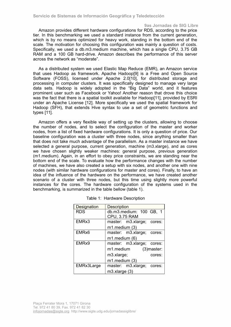
9as Jornadas de SIG LibreAmazon provides different hardware configurations for RDS, according to the price

tier. In this benchmarking we used a standard instance from the current generation,which is by no means optimized for heavy work, standing in the bottom end of thescale. The motivation for choosing this configuration was mainly a question of costs.Specifically, we used a db.m3.medium machine, which has a single CPU, 3.75 GBRAM and a 100 GB hard-drive. Amazon describes the performance of this serveracross the network as “moderate”.

As a distributed system we used Elastic Map Reduce (EMR), an Amazon servicethat uses Hadoop as framework. Apache Hadoop[9] is a Free and Open SourceSoftware (FOSS), licensed under Apache 2.0[10], for distributed storage andprocessing in computer clusters. It was specifically designed to manage very largedata sets. Hadoop is widely adopted in the “Big Data” world, and it featuresprominent user such as Facebook or Yahoo! Another reason that drove this choicewas the fact that there is a spatial toolkit available for Hadoop[11], provided by ESRIunder an Apache License [12]. More specifically we used the spatial framework forHadoop (SFH), that extends Hive syntax to use a set of geometric functions andtypes [11].

Amazon offers a very flexible way of setting up the clusters, allowing to choosethe number of nodes, and to select the configuration of the master and workernodes, from a list of fixed hardware configurations. It is only a question of price. Ourbaseline configuration was a cluster with three nodes, since anything smaller thanthat does not take much advantage of the parallelism. As a master instance we haveselected a general purpose, current generation, machine (m3.xlarge), and as coreswe have chosen slightly weaker machines: general purpose, previous generation(m1.medium). Again, in an effort to obey price constraints, we are standing near thebottom end of the scale. To evaluate how the performance changes with the numberof machines, we have also created a setup with six nodes, and another one with ninenodes (with similar hardware configurations for master and cores). Finally, to have anidea of the influence of the hardware on the performance, we have created anotherscenario of a cluster with three nodes, but this time using slightly more powerfulinstances for the cores. The hardware configuration of the systems used in thebenchmarking, is summarized in the table bellow (table 1).

Table 1: Hardware Description

Designation DescriptionRDS db.m3.medium: 100 GB, 1

CPU, 3.75 RAMEMRx3 master: m3.xlarge; cores:

m1.medium (3)EMRx6 master: m3.xlarge; cores:

m1.medium (6)EMRx9 master: m3.xlarge; cores:

m1.medium (3)master:m3.xlarge; cores:m1.medium (3)

EMRx3Large master: m3.xlarge; cores:m3.xlarge (3)



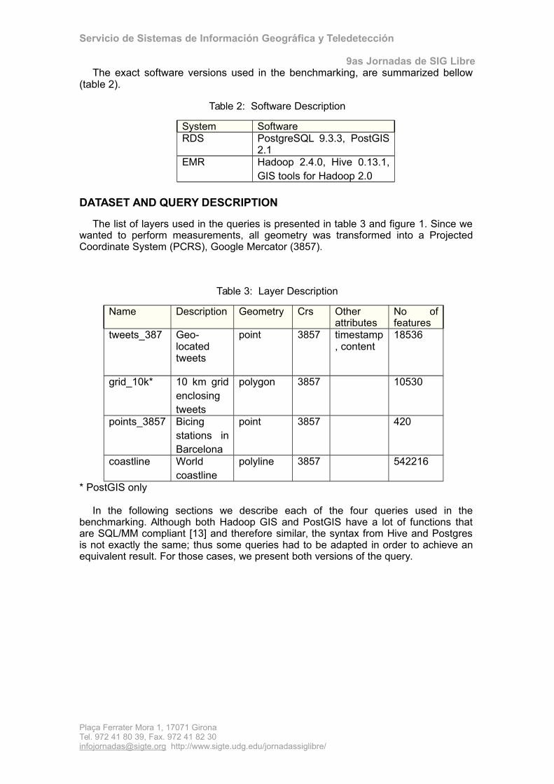
9as Jornadas de SIG LibreThe exact software versions used in the benchmarking, are summarized bellow

(table 2).

Table 2: Software Description

System SoftwareRDS PostgreSQL 9.3.3, PostGIS

2.1EMR Hadoop 2.4.0, Hive 0.13.1,

GIS tools for Hadoop 2.0

DATASET AND QUERY DESCRIPTION

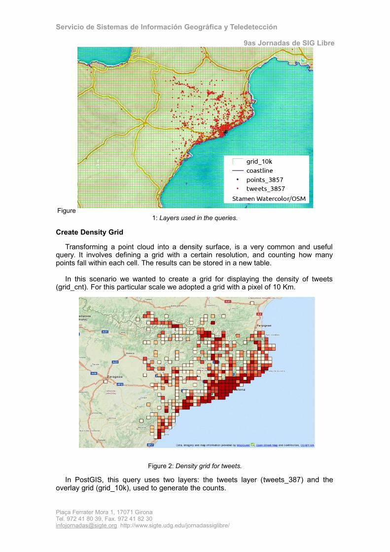
The list of layers used in the queries is presented in table 3 and figure 1. Since wewanted to perform measurements, all geometry was transformed into a ProjectedCoordinate System (PCRS), Google Mercator (3857).

Table 3: Layer Description

Name Description Geometry Crs Otherattributes

No offeatures

tweets_387 Geo-locatedtweets

point 3857 timestamp, content

18536

grid_10k* 10 km gridenclosingtweets

polygon 3857 10530

points_3857 Bicingstations inBarcelona

point 3857 420

coastline Worldcoastline

polyline 3857 542216

* PostGIS only

In the following sections we describe each of the four queries used in thebenchmarking. Although both Hadoop GIS and PostGIS have a lot of functions thatare SQL/MM compliant [13] and therefore similar, the syntax from Hive and Postgresis not exactly the same; thus some queries had to be adapted in order to achieve anequivalent result. For those cases, we present both versions of the query.




Figure1: Layers used in the queries.

Create Density Grid

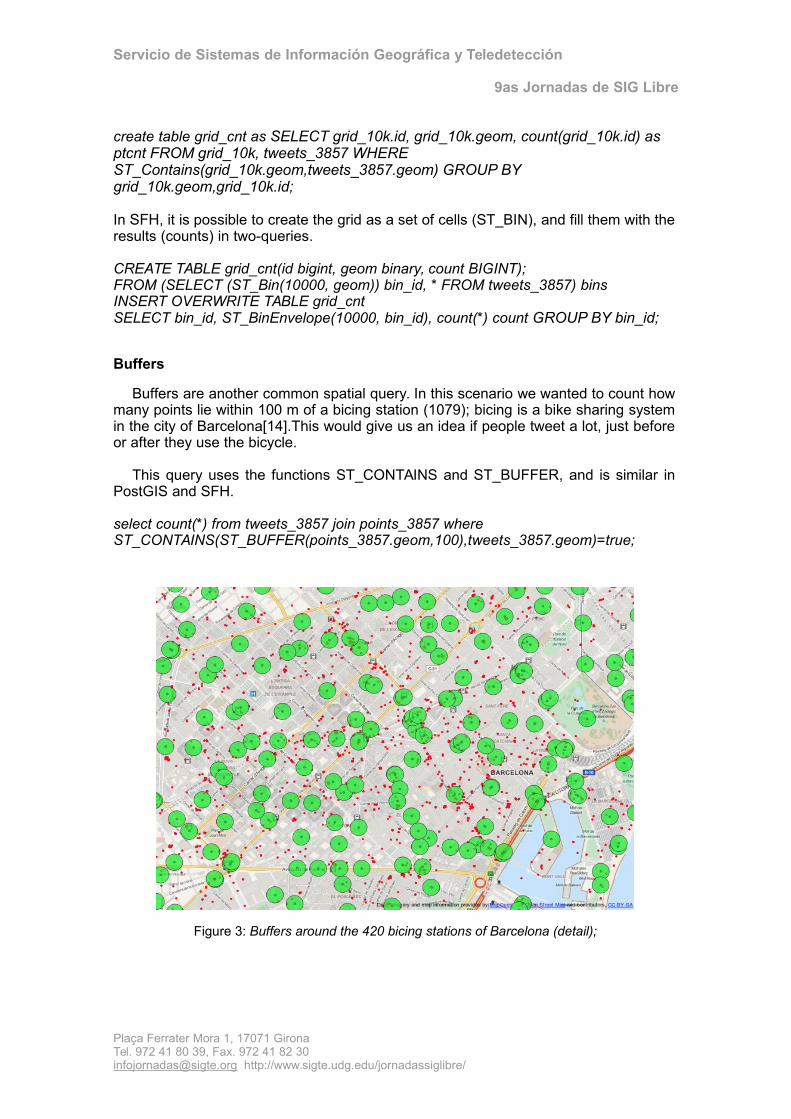
Transforming a point cloud into a density surface, is a very common and usefulquery. It involves defining a grid with a certain resolution, and counting how manypoints fall within each cell. The results can be stored in a new table.

In this scenario we wanted to create a grid for displaying the density of tweets(grid_cnt). For this particular scale we adopted a grid with a pixel of 10 Km.

Figure 2: Density grid for tweets.

In PostGIS, this query uses two layers: the tweets layer (tweets_387) and theoverlay grid (grid_10k), used to generate the counts.




create table grid_cnt as SELECT grid_10k.id, grid_10k.geom, count(grid_10k.id) as ptcnt FROM grid_10k, tweets_3857 WHERE ST_Contains(grid_10k.geom,tweets_3857.geom) GROUP BY grid_10k.geom,grid_10k.id;

In SFH, it is possible to create the grid as a set of cells (ST_BIN), and fill them with theresults (counts) in two-queries.

CREATE TABLE grid_cnt(id bigint, geom binary, count BIGINT);FROM (SELECT (ST_Bin(10000, geom)) bin_id, * FROM tweets_3857) binsINSERT OVERWRITE TABLE grid_cntSELECT bin_id, ST_BinEnvelope(10000, bin_id), count(*) count GROUP BY bin_id;

Buffers

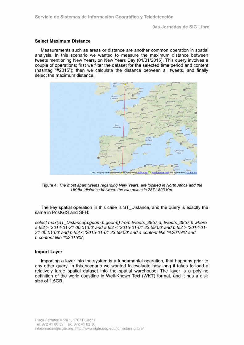
Buffers are another common spatial query. In this scenario we wanted to count howmany points lie within 100 m of a bicing station (1079); bicing is a bike sharing systemin the city of Barcelona[14].This would give us an idea if people tweet a lot, just beforeor after they use the bicycle.

This query uses the functions ST_CONTAINS and ST_BUFFER, and is similar inPostGIS and SFH.

select count(*) from tweets_3857 join points_3857 where ST_CONTAINS(ST_BUFFER(points_3857.geom,100),tweets_3857.geom)=true;

Figure 3: Buffers around the 420 bicing stations of Barcelona (detail);




Select Maximum Distance

Measurements such as areas or distance are another common operation in spatialanalysis. In this scenario we wanted to measure the maximum distance betweentweets mentioning New Years, on New Years Day (01/01/2015). This query involves acouple of operations; first we filter the dataset for the selected time period and content(hashtag “#2015”); then we calculate the distance between all tweets, and finallyselect the maximum distance.

Figure 4: The most apart tweets regarding New Years, are located in North Africa and theUK;the distance between the two points is 2871.893 Km.

The key spatial operation in this case is ST_Distance, and the query is exactly thesame in PostGIS and SFH:

select max(ST_Distance(a.geom,b.geom)) from tweets_3857 a, tweets_3857 b where a.ts2 > '2014-01-31 00:01:00' and a.ts2 < '2015-01-01 23:59:00' and b.ts2 > '2014-01-31 00:01:00' and b.ts2 < '2015-01-01 23:59:00' and a.content like '%2015%' and b.content like '%2015%';

Import Layer

Importing a layer into the system is a fundamental operation, that happens prior toany other query. In this scenario we wanted to evaluate how long it takes to load arelatively large spatial dataset into the spatial warehouse. The layer is a polylinedefinition of the world coastline in Well-Known Text (WKT) format, and it has a disksize of 1.5GB.




Figure 5: World coastline.

The process of importing data from flat files into the system, is relatively different inPostGIS and SFH. In PostGIS we start by creating a table (coastline) to accommodatethe text definitions of the geometry; the next step is to fill it from the file, using the\copy directive; then we add a column to store the geometry and update it,instantiating the geometry from WKT (using ST_GeomFromText).

CREATE TABLE coastline(wkt varchar);\copy coastline from 'coastline.csv' with DELIMITER ' ' CSV QUOTE AS '"' header;alter table coastline add column geom geometry;update coastline set geom=ST_GeomFromText(wkt);

To finalize the definition of the spatial table, we would still need to create a spatialindex and update the SRID of the geometry.

CREATE INDEX idx_coastline_geom ON coastline USING GIST (geom);select updategeometrysrid('coastline','geom', 3857);

On the other hand, the import of the layer into SFH, can be performed in two simplesteps; first we create an external table that maps the WKT value into a string (fromHive 0.14 it is possible to create a TEMPORARY table instead, which will only liveduring that session); then we create a new table that instantiates the geometry fromthat string, at the same time it sets the SRID.

create external table tmp_coastline (wkt string) row format serde 'com.bizo.hive.serde.csv.CSVSerde'with serdeproperties("separatorChar" = "\;","quoteChar" = "\"")stored as textfile LOCATION 's3n://bdigital-benchmarking/coastline/';



9as Jornadas de SIG Librecreate table coastline as select ST_SetSRID(ST_GeomFromText(wkt),3857) as geom from tmp_coastline where WKT NOT LIKE 'WKT';

Note that in both cases the SRID is not optional, since we need it to correctlyperform measurements and relate spatial layers.

Since the most expensive query from this set is the one where we update thegeometry from WKT, in both systems we focused our benchmarking in this query.

DISCUSSION OF RESULTS

We perform each one of the queries presented in the previous section, in ourbenchmarking environments: RDS and the different cluster setups discussed onsection “Benchmarking setup”.

On PostGIS, we run the “explain analyse” function in order to have an idea of whatwas involved in the query, and the estimated time.

On the clusters we noticed a large variability in query time, that could reach asmuch as 20 seconds difference. To limit the influence of this variability in the scope ofthe results, we performed each query 10 times, and used the average value.

On Figure 6, we can see an overview of the results.

Figure 6: Results of the benchmarking of the different queries, on different setups on the cloud;query duration is shown in seconds.

The most expensive query in terms of time, is by far the buffers query. This is alsothe query where the difference in performance between RDS and the clusters ishigher (figure 7). The output of “explain analyse” shows the nested loop involvedwithin ST_CONTAINS as an extremely expensive operation for PostGIS.




Figure 7: Average duration of the buffer query.

The same could be said regarding the import query (figure 8), where the process ofimporting is quite different in PostGIS and the SFH (see section “Dataset and querydescription”). Although the best results are also achieved with the cluster with morepowerful machines (EMRx3Large), this is the only case where, in average, addingmore nodes to the cluster actually results in a gain of performance.

Figure 8: Average duration of the import query.

A discussion on Stack Overflow [15] pointed out some different ways of importinglarge spatial datasets into RDS. The conclusion was that copying features using /copyand update geometry is not the most efficient way; thus for a matter of completeness,we also run an import of an equivalent Shapefile using “shp2pgsql” and the -Ddirective, a method pointed as more efficient. This is the exact query, that in one go,imports the Shapefile into a new table and sets the SRID:

shp2pgsql -D -s 3857 lines.shp coastline | psql -d benchmarking

This query finishes just under 3 minutes (179 s), being faster than the EMRx3cluster.




But RDS is not always slower than the clusters. In creating the density grid, RDS is20 to 50 times faster (figure 8), which could be at least partly explained by the fact thatthe queries are slightly different in both systems.

Figure 8: Average duration of the density grid query.

The cluster with 3 large machines (EMRx3Large) consistently performs better thanthe other clusters in every query, and better than RDS in most queries (with theexception of the density grid). Regarding the other 3 clusters (EMRx3, EMRx6 andEMRx9) the results are not so clear. Generally speaking, there are small differencesbetween the query times in these three setups. In three of the queries (density grid,buffers and distance) there is a small gain in using 6 nodes rather than 3, but using 9workers actually results in larger response times. This could be due to the extraoverhead of marshalling the tasks between clusters.

The distance query (figure 9) is the second less expensive query and in this casePostGIS also performs better than the smaller cluster (EMRx3).

Figure 9: Average duration of the distance grid query.

This benchmarking would not be complete without an analysis of the costs. In orderto extract some practical lessons from these results and evaluate potential solutions,we need to know how much it costs to setup this infra-structure on the cloud.




Figure 10: Cost in dollars, for deploying each benchmarking environment in AWS (1hour/1month).

Amazon uses a model that relies on the type of service, machine, and in the caseof cluster, number of nodes, to calculate the price. The Amazon Web Services PriceCalculator[16] allows us to calculate the exact prices, based on the number of hoursper month that we need to rent the infra structure (figure 10). In this benchmarking allthe queries could be completed in less than one hour, which means we only need touse one hour of each environment.

CONCLUSIONS

These results have a value within their scope: a working benchmarking, buildaround the systems we typically use (low cost), the sample sizes that we commonlyfind (not huge) and the typical operations that we do (measurements, relationshiptests, imports). They cannot be easily extrapolated to huge sample sizes, or morepowerful systems. Nevertheless relevant lessons, some of them not completelyobvious, could be inferred from these experiments.

The first conclusion is that a cluster is not always preferable to a RDBMS. This willactually depend on the query type and we suspect, on the sample size. In theory foran extremely large sample, RDBMS would not work, and much before that thedifferences in performance would start to be noticed; that is not the case for smallersample sizes. This idea is confirmed by the fact that RDS performed better in the leastexpensive queries.

Another conclusion is that adding nodes to a cluster does not necessarily result in abetter performance. In the type of query and sample size used in this benchmarking,often smaller clusters outperformed the cluster with more nodes. Adding more nodesto the system increases the overhead in terms of having to distribute the workload; tocompensate for that the system has to be more efficient, something that can be onlyachieved by taking advantage of the parallelism. One possible explanation is that theSFH is not taking full advantage of the MapReduce paradigm; this should be furtherinvestigated, since it could result in a bottleneck in an Hadoop-based system. On theother hand having a small cluster (3 nodes) with more powerful machines(EMRx3Large), achieved always a better performance. This gain in performance wasmore noticeable than the gain in adding more nodes, when it existed (the queriesresponses for clusters with 3, 6 and 9 nodes were quite similar). This is mostly a gain



9as Jornadas de SIG Librethrough vertical scalability, rather than through horizontal scalability, which is what wewould normally expect from a cluster.

Regarding prices for one hour usage, RDS is much cheaper (about 4x) than thecheapest cluster presented in the benchmarking. Regarding clusters, the system with9 nodes (EMRx9) should be left out, as it is more expensive and it generally does notperform better than the ones with 3 and 6 nodes (EMRx3, EMRx6). The system withmore powerful nodes (EMRx3Large) has a small price difference, that is largelyjustified by its gain in terms of performance.

The differences in query syntax are a reminder that Postgres/PostGIS andHadoop/SFH process things differently, and that alone should force us to evaluatecarefully which option is more appropriated for the particular problem we are dealingwith.

REFERENCES

Dunning, T. and Friedman, E. (2014) Time Series Databases: New Ways to Storeand Access Data. O'Reilly Media; 1 edition.

OpenStreetMap. OpenStreetMap. Retrieved March 9, 2015, from:https://www.openstreetmap.org/

Ushahidi. Ushahidi. Retrieved March 9, 2015, from: http://www.ushahidi.com/ Aji, A.; Wang, F.; Vo, H.; Lee, R.; Liu, Q.; Zhang, X. & Saltz, J. (2013). Hadoop-

GIS: A High Performance Spatial Data Warehousing System over MapReduce.Proceedings of the VLDB Endowment International Conference on Very LargeData Bases, 6(11), p1009.

Amazon. Amazon Web Services. Retrieved March 15, 2015, from:https://aws.amazon.com/

PostgreSQL. PostgreSQL. Retrieved March 15, 2015, from:http://www.postgresql.org/

License. PostgreSQL. Retrieved March 9, 2015, from:http://www.postgresql.org/about/licence/

PostGIS. Spatial and Geographic objects for PostgreSQL. Retrieved March 9,2015, from: http://postgis.net/

Apache. Hadoop. Retrieved March 9, 2015, from: https://hadoop.apache.org/ The Apache Software Foundation. Apache License, Version 2.0. Retrieved March

15, 2015, from: http://www.apache.org/licenses/LICENSE-2.0 ESRI. Spatial Framework for Hadoop. Retrieved March 15, 2015, from:

https://github.com/Esri/spatial-framework-for-hadoop ESRI. Spatial Framework for Hadoop license. Retrieved March 15, 2015, from:

https://github.com/Esri/spatial-framework-for-hadoop/blob/master/license.txt Stolze, K. SQL/MM Spatial: The Standard to Manage Spatial Data in Relational

Database Systems. Retrieved March 15, 2015, from: http://doesen0.informatik.uni-leipzig.de/proceedings/paper/68.pdf

Wikipedia. Bicing. Retrieved March 15, 2015, from:https://en.wikipedia.org/wiki/Bicing

Stack Overflow. What is the best hack for importing large datasets into PostGIS?Retrieved March 9, 2015, from:http://gis.stackexchange.com/questions/109564/what-is-the-best-hack-for-importing-large-datasets-into-postgis

Amazon Web Services. Simple Monthly Calculator. Retrieved March 9, 2015, fromhttps://calculator.s3.amazonaws.com/index.html


https://calculator.s3.amazonaws.com/index.html

http://gis.stackexchange.com/questions/109564/what-is-the-best-hack-for-importing-large-datasets-into-postgis

http://gis.stackexchange.com/questions/109564/what-is-the-best-hack-for-importing-large-datasets-into-postgis

https://en.wikipedia.org/wiki/Bicing

http://doesen0.informatik.uni-leipzig.de/proceedings/paper/68.pdf

http://doesen0.informatik.uni-leipzig.de/proceedings/paper/68.pdf

https://github.com/Esri/spatial-framework-for-hadoop/blob/master/license.txt

https://github.com/Esri/spatial-framework-for-hadoop

http://www.apache.org/licenses/LICENSE-2.0

https://hadoop.apache.org/

http://postgis.net/

http://www.postgresql.org/about/licence/

http://www.postgresql.org/

https://aws.amazon.com/

http://www.ushahidi.com/

https://www.openstreetmap.org/

Big Data y Bases de Datos Espaciales: un análisis ... - UdG

Documents

Transcript of Big Data y Bases de Datos Espaciales: un análisis ... - UdG