A&A 645, A127 (2021)https://doi.org/10.1051/0004-6361/202039544c© GRAVITY Collaboration 2021

Astronomy&Astrophysics

Detection of faint stars near Sagittarius A* with GRAVITYGRAVITY Collaboration?: R. Abuter8, A. Amorim6,12, M. Bauböck1, J. P. Berger5,8, H. Bonnet8, W. Brandner3,

Y. Clénet2, Y. Dallilar1, R. Davies1, P. T. de Zeeuw10,1, J. Dexter13,1, A. Drescher1,16, F. Eisenhauer1,N. M. Förster Schreiber1, P. Garcia7,12, F. Gao1,??, E. Gendron2, R. Genzel1,11, S. Gillessen1, M. Habibi1,

X. Haubois9, G. Heißel2, T. Henning3, S. Hippler3, M. Horrobin4, A. Jiménez-Rosales1, L. Jochum9, L. Jocou5,A. Kaufer9, P. Kervella2, S. Lacour2, V. Lapeyrère2, J.-B. Le Bouquin5, P. Léna2, D. Lutz1, M. Nowak15,2, T. Ott1,T. Paumard2,??, K. Perraut5, G. Perrin2, O. Pfuhl8,1, S. Rabien1, G. Rodríguez-Coira2, J. Shangguan1, T. Shimizu1,S. Scheithauer3, J. Stadler1, O. Straub1, C. Straubmeier4, E. Sturm1, L. J. Tacconi1, F. Vincent2, S. von Fellenberg1,

I. Waisberg14,1, F. Widmann1, E. Wieprecht1, E. Wiezorrek1, J. Woillez8, S. Yazici1,4, and G. Zins9

1 Max Planck Institute for extraterrestrial Physics, Giessenbachstraße 1, 85748 Garching, Germany2 LESIA, Observatoire de Paris, Université PSL, CNRS, Sorbonne Université, Université de Paris, 5 place Jules Janssen,

92195 Meudon, France3 Max Planck Institute for Astronomy, Königstuhl 17, 69117 Heidelberg, Germany4 1st Institute of Physics, University of Cologne, Zülpicher Straße 77, 50937 Cologne, Germany5 Univ. Grenoble Alpes, CNRS, IPAG, 38000 Grenoble, France6 Universidade de Lisboa – Faculdade de Ciências, Campo Grande, 1749-016 Lisboa, Portugal7 Faculdade de Engenharia, Universidade do Porto, rua Dr. Roberto Frias, 4200-465 Porto, Portugal8 European Southern Observatory, Karl-Schwarzschild-Straße 2, 85748 Garching, Germany9 European Southern Observatory, Casilla 19001, Santiago 19, Chile

10 Sterrewacht Leiden, Leiden University, Postbus 9513, 2300 RA Leiden, The Netherlands11 Departments of Physics and Astronomy, Le Conte Hall, University of California, Berkeley, CA 94720, USA12 CENTRA – Centro de Astrofísica e Gravitação, IST, Universidade de Lisboa, 1049-001 Lisboa, Portugal13 Department of Astrophysical & Planetary Sciences, JILA, Duane Physics Bldg., University of Colorado, 2000 Colorado Ave,

Boulder, CO 80309, USA14 Department of Particle Physics & Astrophysics, Weizmann Institute of Science, Rehovot 76100, Israel15 Institute of Astronomy, Madingley Road, Cambridge CB3 0HA, UK16 Department of Physics, Technical University Munich, James-Franck-Straße 1, 85748 Garching, Germany

Received 28 September 2020 / Accepted 4 November 2020

ABSTRACT

The spin of the supermassive black hole that resides at the Galactic Center can, in principle, be measured by accurate measurementsof the orbits of stars that are much closer to Sgr A* than S2, the orbit of which recently provided the measurement of the gravitationalredshift and the Schwarzschild precession. The GRAVITY near-infrared interferometric instrument combining the four 8m telescopesof the VLT provides a spatial resolution of 2–4 mas, breaking the confusion barrier for adaptive-optics-assisted imaging with a sin-gle 8–10m telescope. We used GRAVITY to observe Sgr A* over a period of six months in 2019 and employed interferometricreconstruction methods developed in radio astronomy to search for faint objects near Sgr A*. This revealed a slowly moving star ofmagnitude 18.9 in the K-band within 30 mas of Sgr A*. The position and proper motion of the star are consistent with the previouslyknown star S62, which is at a substantially greater physical distance, but in projection passes close to Sgr A*. Observations in Augustand September 2019 detected S29 easily, with K-magnitude of 16.6, at approximately 130 mas from Sgr A*. The planned upgradesof GRAVITY, and further improvements in the calibration, offer greater chances of finding stars fainter than K-magnitude of 19.

Key words. Galaxy: center – stars: imaging – infrared: stars

1. Introduction

The Galactic Center (GC) excels as a laboratory for astrophysicsand general relativity (GR) around a massive black hole (MBH;

? GRAVITY was developed as part of a collaboration by the MaxPlanck Institute for extraterrestrial Physics, LESIA of the Observatoirede Paris/Université PSL/CNRS/Sorbonne Université/Université de Parisand IPAG of Université Grenoble Alpes/CNRS, the Max Planck Insti-tute for Astronomy, the University of Cologne, the CENTRA – Centrode Astrofisica e Gravitação, and the European Southern Observatory.?? Corresponding authors: F. Gao, e-mail: fgao@mpe.mpg.de;T. Paumard, e-mail: thibaut.paumard@obspm.fr

Genzel et al. 2010). The observation of stellar orbits in the GCaround the radio source Sgr A* (Eckart & Genzel 1996; Ghezet al. 1998, 2003, 2008; Schödel et al. 2002; Gillessen et al.2009, 2017) has opened a route to testing gravity in the vicin-ity of an MBH with clean test particles. The gravitational red-shift from Sgr A* has been detected at high significance inthe spectrum of the star S2 during the 2018 pericenter pas-sage of its 16-year orbit (GRAVITY Collaboration 2018a, 2019;Do et al. 2019). Recently, the relativistic Schwarzschild pre-cession of the pericenter has also been detected in S2’s orbit(GRAVITY Collaboration 2020a). The effects detected are oforder β2, where β = v/c (Zucker et al. 2006). It is not clear,

Open Access article, published by EDP Sciences, under the terms of the Creative Commons Attribution License (https://creativecommons.org/licenses/by/4.0),which permits unrestricted use, distribution, and reproduction in any medium, provided the original work is properly cited.

Open Access funding provided by Max Planck Society.

A127, page 1 of 10

A&A 645, A127 (2021)

however, whether higher order effects such as the Lense-Thirringprecession due to the spin of the black hole can be detected inthe orbit of S2, since these fall off faster with distance from theMBH. In addition, stars located farther away from Sgr A* aremore affected by Newtonian perturbations by surrounding starsand dark objects, which can make a spin measurement with S2more difficult (Merritt et al. 2010; Zhang & Iorio 2017). Hence,it is natural to look for stars at smaller radii. In particular, sucha star could offer the possibility of measuring Sgr A*’s spin(Waisberg et al. 2018). If it were possible to additionally measurethe quadrupole moment of the MBH independently, the relationbetween these two parameters would constitute a test of the no-hair theorem of GR (Will 2008; Waisberg et al. 2018).

Beyond the purpose of testing GR, the GC cluster is the mostimportant template for galactic nuclei. These are the sites ofextreme mass ratio inspirals (Amaro-Seoane et al. 2007), whichis one of the source categories for the gravitational wave obser-vatory LISA (Baker et al. 2019). Understanding the GC clusterdown to the smallest possible scales delivers important anchorpoints for understanding the structure and dynamics of these stel-lar systems, and thus for predictions of the expected event rates.

The number of stars expected at smaller radii has until nowbeen estimated by extrapolating the density profile in the GC toradii smaller than the resolution limit of ∼60 mas in the near-infrared provided by 8–10 m class telescopes and extrapolatingthe mass function to stars fainter than the confusion limit in thecentral arcsecond around mK ≈ 18. Both functions have beendetermined in the literature (Genzel et al. 2003b; Do et al. 2013;Gallego-Cano et al. 2018), and the resulting estimate for thenumber of stars suitable for GR tests is of order 1 (Waisberget al. 2018).

The near-infrared interferometric instrument GRAVITY(GRAVITY Collaboration 2017) mounted on the four 8m tele-scopes of the VLT makes it possible to detect and trace such faintstars for the first time with an angular resolution that exceedsthat of adaptive-optics-assisted imaging on 8–10 m telescopesby a factor of ∼20. Here, we report on the detection of a faintstar (mK ≈ 18.9) within 30 mas of Sgr A*. We used the classicalradio interferometry data-reduction/image-reconstruction pack-age, Astronomy Image Process Software (AIPS; Greisen 2003)for our work. This detection does not yet explore the signal-to-noise ratio limit of GRAVITY, but is limited by our abilityto model the point spread function (PSF) of the sparse four-telescope interferometer and the presence of other sources andtheir sidelobes in the field of view (FOV).

This paper is organized as follows. We describe our observa-tions in Sect. 2. Then, in Sect. 3, we describe in detail the data-reduction and image-reconstruction process to derive the images,with Sgr A* removed. We show the faint star detection in Sect. 4,together with validation from model fitting and constraints on theproper motion of the detected star. We cross-check our detectionwith the expected positions of known S-stars and also give thelimitation of our current imaging technique in Sect. 5. Finally,we give our conclusions in Sect. 6.

2. Observations

We observed Sgr A* and the immediate surroundings (Fig. 1)using the VLT/GRAVITY instrument at the ESO Paranal Obser-vatory between 2019 March 27 and 2019 September 15, underGTO programs 0102.B-0689 and 0103.B-0032, spread over atotal of 28 nights. The data are the same as those used inGRAVITY Collaboration (2020a). Compared to the 2017 and2018 data on the Galactic Center, the 2019 data have the

S1

S2S4

S8

S9

S12

S13

S14

S17

S18

S19S21

S23

S24

S29

S31

S33

S38

S42

S54

S55

S60

S71

S175

S5

S6

S7

S10

S11

S20

S22

S25

S26

S27

S28

S30

S32

S34S35

S36

S37

S39

S41

S43

S44

S45

S46

S47

S48

S50

S51

S52

S53

S56

S57

S58

S59

S62

S63

S64

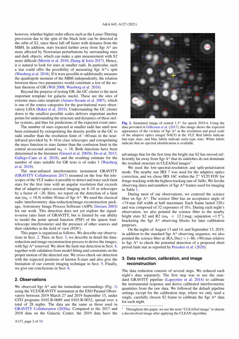
Fig. 1. Simulated image of central 1.3′′ for epoch 2019.4. Using thedata provided in Gillessen et al. (2017), this image shows the expectedappearance of the vicinity of Sgr A* at the resolution and pixel scaleof the adaptive optics imager NACO at the VLT. Red labels indicatelate-type stars, and blue labels indicate early-type stars. White labelsindicate that no spectral identification is available.

advantage that for the first time the bright star S2 has moved suf-ficiently far away from Sgr A* that its sidelobes do not dominatethe residual structure in CLEANed images1.

We used the low-spectral-resolution and split-polarizationmode. The nearby star IRS 7 was used for the adaptive opticscorrection, and we chose IRS 16C within the 2′′ VLTI FOV forfringe-tracking with the highest tracking rate of 1kHz. We list theobserving dates and numbers of Sgr A* frames used for imagingin Table 1.

During most of our observations, we centered the sciencefiber on Sgr A*. The science fiber has an acceptance angle of≈74 mas full width at half maximum. Each frame lasted 320 sand was composed of 32 exposures of 10 s. During each night’sobservation, we also pointed the science fiber to the nearbybright stars S2 and R2 (mK ≈ 12.1 mag; separation ≈1.5′′),bracketing the Sgr A* observing blocks for later calibrationpurposes.

On the nights of August 13 and 14, and September 13, 2019,in addition to the standard Sgr A* observing sequence, we alsopointed the science fiber at (RA,Dec) ≈ (−86,+90) mas relativeto Sgr A* to check the potential detection of a proposed shortperiod faint star as reported by Peissker et al. (2020).

3. Data reduction, calibration, and imagereconstruction

The data reduction consists of several steps. We reduced eachnight’s data separately. The first step was to use the stan-dard GRAVITY pipeline (Lapeyrère et al. 2014) to calibratethe instrumental response and derive calibrated interferometricquantities from the raw data. We followed the default pipelinesettings except for the calibration step, where we only used asingle, carefully chosen S2 frame to calibrate the Sgr A* datafor each night.

1 Throughout this paper, we use the term “CLEANed image” to denotea deconvolved image after applying the CLEAN algorithm.

A127, page 2 of 10

GRAVITY Collaboration: Detection of faint stars near Sagittarius A* with GRAVITY

Table 1. Observation details.

Date Nobs Nused Incl.

2019-03-27 6 0 N2019-03-28 8 0 N2019-03-30 2 0 N2019-03-31 5 0 N2019-04-15 8 0 N2019-04-16 4 0 N2019-04-18 17 17 Y2019-04-19 12 10 Y2019-04-21 28 11 N2019-06-13 4 0 N2019-06-14 4 0 N2019-06-16 17 4 N2019-06-17 5 0 N2019-06-18 4 0 N2019-06-19 8 6 N2019-06-20 27 15 Y2019-07-15 8 7 Y2019-07-17 39 32 Y2019-08-13 21 21 Y2019-08-14 10 8 Y2019-08-15 25 25 Y2019-08-17 8 0 N2019-08-18 18 14 Y2019-08-19 21 15 Y2019-09-11 9 8 Y2019-09-12 14 8 Y2019-09-13 11 5 Y2019-09-15 12 10 Y

Notes. Observation details. Here we list all the Sgr A* observationstaken in 2019, together with the number of frames observed (Nobs),number of frames used per image per night (Nused), and whether theyare included in the final image per month. Each frame is 32 secondslong.

3.1. Data format conversion

The standard GRAVITY data products are stored in the OIFITSformat after calibration (Duvert et al. 2017). In order to benefitfrom existing radio interferometry imaging reconstruction soft-ware and algorithms, we converted the GRAVITY data productsinto the UVFITS format (Greisen 2016), which is commonlyused in radio interferometry.

The conversion was done with a python script thatwe adapted from the EHT-imaging package (Event HorizonTelescope Collaboration 2019). The essential data we readfrom the calibrated OIFITS files are the VISAMP, VISPHI,MJD, and UV coordinates (UCOORD, VCOORD) columnsfrom the OI_VIS table for the science channel output togetherwith the corresponding OI_FLUX table. We then rewrote thesefollowing the UVFITS format convention. We also took theOI_WAVELENGTH table and wrote it into the FQ table usedin UVFITS. Since the effective bandwidth for each wavelengthoutput is different, we put each wavelength output as an inde-pendent intermediate frequency (IF) rather than an independentchannel in the UVFITS file.

3.2. Additional amplitude calibration

Before writing out the UVFITS data product, we re-calibratedand re-scaled the visibility amplitudes with the photometric flux

of each baseline calculated from each telescope pair (using theOI_FLUX table). This gave us the correlated flux from eachbaseline instead of the default normalized visibility, which doesnot reflect the true brightness of the target. During this step, wealso corrected for the attenuation of the telescope flux due to dif-ferent air mass and AO correction by fitting a polynomial func-tion to the OI_FLUX of several S2 frames per telescope acrossone night and interpolating the correction per telescope accord-ingly.

We then re-normalized each visibility amplitude with that ofthe S2 frame used for calibration in the previous step. Thus,our visibility amplitudes are normalized such that a visibilityamplitude of 1 equals S2’s magnitude in the Ks band (mK = 14.1,Gillessen et al. 2017).

The final VIS_AMP quantity we wrote out is

aobj(t)i j,final = aobj(t)

i j

√fi(t) f j(t)σi(t)σ j(t)

fi(t0) f j(t0)σi(t0)σ j(t0), (1)

where aobj(t)i j is the pipeline-produced visibility amplitude of a

certain target frame at time t between telescope i and j, fi(t) isthe measured flux from telescope i at time t, and σi(t) is thefit air mass correction coefficient for telescope i at time t. Thetime t0 corresponds to the S2 frame used for calibration in theGRAVITY pipeline.

3.3. Image reconstruction and deconvolution with CLEAN

After the data reduction steps, we loaded the calibrated andamplitude re-normalized complex visibility data into AIPS forimage reconstruction with the task IMAGR. Sgr A* is known toexhibit variability on a timescale of minutes in the near-infrared(Genzel et al. 2003a; Ghez et al. 2004; Gillessen et al. 2006;Eckart et al. 2008; Do et al. 2009; Dodds-Eden et al. 2011;Witzel et al. 2018; GRAVITY Collaboration 2020a,b). This vari-ability must be taken into account during image reconstructionin order to remove, as much as possible, the sidelobes of Sgr A*,which dominate the residual map and limit the sensitivity. Wereduced the impact of the variability by reconstructing each 320-second-long frame individually. While the variability on thistimescale can be high during flares, it is much lower during qui-escent phases. Consequently, we assumed the flux to be constantover the duration of each frame.

In the spectral domain, we only included data from 2.111 µmto 2.444 µm in order to minimize systematic biases from theedge channels, which are subject to increased instrumental (shortwavelengths) and thermal (long wavelengths) background. Weused the data from both polarizations (as Stokes I) in the recon-struction of the images. Given that our synthesized beam size isabout 2 × 4 mas, we chose a pixel size of 0.8 mas and an imagesize of 512×512 pixels, which can fully cover the fiber FOV witha FWHM of about 74 mas. When applying CLEAN to the Sgr A*frames, we applied a spectral index of +62. The IMAGR taskrequires the user to choose the data weighting via a parameter

2 We only kept frames where Sgr A* is relatively faint for later anal-ysis, in which case Sgr A* is expected to have a near-infrared spectralindex (νLν ∼ να) between −3 and −1 (Genzel et al. 2010; Witzel et al.2018). Since we used S2 data to normalize the Sgr A* data, we took intoaccount a spectral index of +2 from the Rayleigh-Jeans approximationof the black-body radiation from S2: this would give us a spectral indexrange of α − 1 between −6 and −4. We then chose the value of −6 so asto cover the extreme cases, and finally we flipped the sign to follow thespectral index definition in AIPS to get the +6 value.

A127, page 3 of 10

A&A 645, A127 (2021)

Fig. 2. (a) Galactic Center region of 5× 5 arcsec as seen by NACO at 2.2 micron. The central white box indicates the region shown in panel b.(b) Image of GC region of 0.8× 0.8 arcsec from the GRAVITY acquisition camera in H-band. The central white box indicates the region shown inpanel c. (c) Image of central 240× 240 mas region with Sgr A* deconvolved with the CLEAN algorithm and overlaid on the residual background.The dashed circles in both panels b and c indicate the GRAVITY fiber FOV with a HWHM of ∼74 mas. S2 was outside of this region and its fluxwas reduced by fiber damping by about a factor of 100.

called ROBUST, which we set to zero. This ensures a balancedresult between natural and uniform weighting. The outputs atthis stage are so-called dirty images, which in theory are the con-volution of the source distribution with the beam pattern.

We now describe the procedure we found to be effectivefor creating residual images in which we can identify addi-tional sources beyond Sgr A*, from the dirty images. Firstly,regarding CLEAN per 320-second frame, we used a small pre-defined clean box centered on Sgr A* – the central and bright-est spot – with a size of 5 × 6 pixels (i.e., smaller than thespatial periodicity of the beam pattern and thus avoiding anysidelobes). We ran CLEAN for multiple iterations until the firstnegative CLEAN component appeared. We repeated the sameprocess for all the frames for a certain night to obtain a seriesof CLEANed images and residual images. Secondly, regardingframe selection, we then visually checked the CLEANed imageand the residual image against the following two criteria: 1) theCLEANed image should show no signs of abnormal instrumen-tal behavior or strong baseline pattern for a specific baseline;2) the peak value of the residual image should be below 0.8 mJy.Due to the limited dynamic range we can reach with the CLEANalgorithm here, the second criterion limits us to those frameswhere Sgr A* is relatively faint (below ∼2 mJy). Thirdly, regard-ing the subtraction of Sgr A*, we subtracted the respectiveCLEAN component model from each frame in the visibilitydomain with the AIPS task UVSUB. And finally, we grouped thedata according to individual nights and combined them in the UVdomain with the AIPS task DBCON. Then, we re-imaged themto get Sgr A*-removed images per night. Before we combinedthe data per month, we first cross-checked these images with thecriteria mentioned in the next section.

We note that we also tried to clean the images after applyingthe phase-only self-calibration by using the task CALIB. How-ever, this did not improve our residual image in general, so noself-calibration was included in our data reduction process. Asan example, in Fig. 2 we show the GC region as observed by theVLT NACO instrument, the GRAVITY acquisition camera, andone Sgr A* reconstructed image.

3.4. Sanity checks

Apart from imaging Sgr A* frames, we also repeated the sameimaging procedure on S2 frames and R2 frames for each night

(with a spectral index of 0) as a sanity check for the instrumentbehavior. This allowed us to check our flux calibration as themagnitude of both S2 and R2 are known and they are not vari-able. Additionally, we can use these data to gauge the dynamicrange we were able to reach with our method and compare thatto the Sgr A* frames.

4. Results

4.1. Source identification

We first estimate, in Sect. 4.1.1, how much on-sky movement wemight expect from a star close to Sgr A*, which puts a limit onhow much data we can combine in time before our images aresmeared. Then, we describe the image co-adding in Sect. 4.1.2.

4.1.1. Prerequisite for the movement of a tentative star

A star belonging to the Sgr A* system is gravitationally bound tothe massive black hole, and hence it is useful to know the escapevelocity for stars within our FOV. For a star located 10 mas awayfrom Sgr A*, the escape velocity is ≈104 km s−1, correspondingto ≈250 mas yr−1. The day-to-day motion of the star on the sky isbelow 0.7 mas, and below 20 mas from month to month. Hence,a tentative star should show up in the images of multiple nights ina month in the same position, given that our synthesis beam sizeis about 2× 4 mas. From one month to the next, the star mightmove at most by a few times the beam size. We can thus co-addthe frames per month.

4.1.2. Co-adding

At this stage, we have a series of Sgr A*-removed imagesper night for March, April, June, July, August, and Septemberin 2019. We first cross-checked the multiple images for eachmonth, knowing that a real source would not move between thenights within a given month. We de-selected frames that visu-ally deviate strongly from the monthly sample. This is a veryhelpful selection criterion, since the total number of Sgr A*frames per night varies greatly, and we do not always reach thesame sensitivity level. Since we reset our instrument every night,instrumental misbehavior or bad observing conditions are morelikely to affect the image from a single night only. Finally, we

A127, page 4 of 10

GRAVITY Collaboration: Detection of faint stars near Sagittarius A* with GRAVITY

Fig. 3. Top row: (a) three-color composite image of the full 200 mas region for the image reconstruction from the April 2019 data, shown asa typical example. Here, Sgr A* (located at the image center) and S2 are color-coded in green, other potential targets are shown in red, and theresidual map is shown in blue. The central white box indicates the central 100 mas region shown in other panels. (b) Stacking of the central 100 masregion around Sgr A* for April, June, July, August, and September 2019. The central bright spot at [0, 0] mas is Sgr A*, with its flux reduced40 times. (c) Image from each month is shown in a different color, illustrating the motion in the south-east direction. Bottom row: three-colorcomposite images of the central 100 mas region around Sgr A* for April, June, July, August, and September in 2019. In each map, Sgr A* iscolor-coded in green, other potential targets are shown in red, and the residual map is shown in blue. North is up and east to the left. S2 is outsideof this region. We highlight the newly detected object with a white circle.

averaged the remaining images in the UV domain to derive thebest Sgr A*-removed image per month, which is shown in Fig. 3.

We tried to run the CLEAN algorithm on these Sgr A*-removed images, on both the manually and automaticallyselected peak positions. However, the CLEAN algorithm didnot finish successfully in several instances, and hence we werenot able to robustly CLEAN these images. We speculate thatthis is because the dirty image pattern on the Sgr A*-removedimages sometimes shows distortion due to time-variable sys-tematic errors, which prevent the CLEAN algorithm from con-verging. Hence, we kept these Sgr A*-removed, but not fur-ther deconvolved images for a manual analysis in the nextstep.

4.2. Inspection of monthly co-adds

The monthly co-added images show multiple patches with somebright features embedded. These are a combination of any targetsin the field convolved with our interferometric beam plus theinterferometric residual background.

The most prominent bright feature on these images is the oneto the northeast of Sgr A*, which is the star S2 (with the distort-ing effect from bandwidth smearing, and a brightness dampedby our fiber profile). Despite its distance exceeding the nominalFOV of GRAVITY, S2 is very robustly detected in all images.

Besides S2, we noticed a bright feature to the north-west ofSgr A* consistently showing up in all our images. This secondmost prominent feature over the sample of images correspondsto another star, as we show below. We performed a 2D Gaussianfit on this bright feature to obtain the position and brightnessrelative to Sgr A* (see Table 2).

SinceweusedS2framestore-normalize theSgrA*frames, thetarget brightness is also normalized to S2. The relative brightnessof this tentative star is 0.0084 ± 0.0009, which is 119 ± 16 times,or 5.2 ± 0.1 magnitudes fainter than S2, a 14.1 magnitude sourcein K-band Gillessen et al. (2009). The detected object is about 27mas away from Sgr A*, which corresponds to a fiber-damping loss(described by a Gaussian function with a FWHM of 74 mas) of≈30%. Taking this effect into account, the intrinsic brightness ofthis object is mK = 18.9 ± 0.1.

4.3. Limiting magnitude in our images

To estimate the noise level on the final best Sgr A*-removedresidual image per month, we selected the central 74 mas×74 mas region of each image, which corresponds to the FWHMof the fiber FOV and also blanked out the 5× 5 mas regionaround the peak of our newly detected star. We then quotethe root-mean-square (rms) calculated in this region as the1-σ noise level for the residual image. S2 is located outside ofthis region, so it does not affect the noise calculation here. Wereport these numbers in Table 2. As the flux in our images isnormalized to S2, so is the 1-σ noise level. We find a mean noiselevel of 1.7 ± 0.2 × 10−3 in relative brightness, corresponding tomK = 21.0 ± 0.2. This is the statistical limit corresponding tothe brightness of a star that would create a peak in our imagescomparable to the noise floor in the absence of systematics. Fora 5-σ detection, an object would need to be at least as bright asmK = 19.3 ± 0.2 if no systematics were present. We note herethat these numbers are “apparent” magnitudes, in the sense thatno fiber damping effects have been considered. Therefore, thereal magnitude of the star for a 5-σ detection should be between

A127, page 5 of 10

A&A 645, A127 (2021)

Table 2. Fit position and relative brightness of the faint star.

Date of the δ RA δ RA err. δ Dec δ Dec err. Relative Relative 1-σ Number ofaveraged image (mas) (mas) (mas) (mas) brightness brightness of S2 noise level frames used

2019.30 (Apr.18) −19.18 0.18 20.78 0.27 0.009 0.013 0.0019 272019.47 (Jun.19) −18.78 0.14 19.80 0.23 0.009 0.011 0.0018 152019.54 (Jul.17) −18.62 0.26 19.73 0.30 0.007 0.009 0.0017 392019.62 (Aug.16) −18.49 0.11 19.88 0.29 0.008 0.009 0.0014 832019.70 (Sep.12) −18.14 0.15 19.57 0.34 0.009 0.011 0.0017 31

Notes. Fit position of our detected target relative to Sgr A* and the image noise level for the best Sgr A*-removed image per month. The positivesign signals the east and north of Sgr A* in the right ascension and declination directions, respectively. The brightness level is a normalizedquantity, with the maximum unity, which corresponds to the brightness of S2, if it were in the field center. Here, the brightness levels do not reflectthe physical brightness of the stars, as they are also affected by bandwidth smearing and fiber damping.

18.5 and 19.3 magnitude, depending on the distance to the centerof the field.

4.4. Interferometric model fit of the data

Since the star we detected is just above the 5-σ detection level,we used the Meudon model-fitting code as an independent wayof verifying that our detection is real. This code was already usedin our papers on the orbit of S2 (GRAVITY Collaboration 2018a)and is able to fit two or three sources.

Our image reconstruction relies on the complex visibilities,that is, the amplitude and phase. The model fit, on the other hand,uses closure amplitudes and phases, giving equal weight to each.

We selected the same frames as for the image reconstructionand fit the frames from each night together, but we separated thetwo polarisation states. For each night, we fit one flux per filefor Sgr A*, one flux per file and per telescope for S2, a singlebackground flux, a spectral index for Sgr A*, and a single posi-tion for S2 and the third source, respectively (neglecting propermotion over the course of the night). S2, the third source, andthe background, are assumed to have a common spectral index,which is fixed.

Blindly starting such a fit would very likely not find the bestminimum, and hence we fed the fitting routine with starting val-ues derived from our imaging. We applied a simple χ2 minimiza-tion algorithm to explore the parameter space in the ±10 masregion around the position of the star derived from imaging.

In all cases, the fits recovered the third star. The reduced χ2 isof the order 2–3. Comparing the Bayesian information criterion(BIC) of the fits with and without the third source strongly sup-ports its presence, and the third source is consistently found atthe position revealed by the imaging reconstruction to within theuncertainties. For example, for the night of April 18, 2019, usingpolarization state P1, the triple-source model yields a reducedχ2 of 2.1 and a BIC of 493, while the binary model yields areduced χ2 of 2.9 and a BIC of 664. ∆BIC is thus 171. The sig-nificance of the detection estimated as flux over uncertainty ofthe third source is 9.6σ. The polarization P2 yields similar sta-tistical estimators. We note that the improvement achieved byfitting three stars instead of two stars is not obvious within afive-minute frame, but only for a full night of data.

4.5. Further checks

To further verify our detection, we also reconstructed images foreach (linear) polarization channel of GRAVITY separately. Our

newly detected star appears in both channels, indicating an originfrom the sky rather than a noise artifact.

We further ran the CLEAN process on Sgr A* (for whichthe spectral index is only poorly constrained) using a spectralindex of zero, and we can still recover the newly detected starin the residual images. Since we only removed Sgr A*, any dif-ference between using different spectral indices must come fromsidelobes and beam patterns related to Sgr A*. This is especiallyhelpful when there are fewer than ten frames available for a cer-tain night.

We can also rule out that the detection is caused by the over-lap of sidelobes from S2 and Sgr A*. As shown in the appendix,three out of six baseline patterns are oriented in the southeast-northwest direction, and one baseline pattern is oriented in thenortheast-southwest direction. In principle, these baseline pat-terns could mimic a detection. However, since S2 is movingaway from Sgr A*, any fake target formed in this way shouldalso move away from Sgr A* in parallel to S2’s motion. This isinconsistent with the star showing up at (almost) the same posi-tion over five months.

4.6. Motion on the sky of the star

We show the change in position of our newly detected star as afunction of time in Fig. 4. We see regular changes in both RightAscension (RA) and Declination (Dec) with time, and a simplelinear fitting (shown in solid line) gives a proper motion in RA of2.38 ± 0.29 mas yr−1 and in Dec of −2.74 ± 0.97 mas yr−1.

We list the proper motions measured based on the positionsderived from the model-fitting method in Table 3. These resultsare within 4-σ uncertainties of the image-based results.

4.7. Tentative detection from 2018 data

Due to the relatively small proper motion of our newly detectedstar, we predict that it is also located inside our FOV in the2017 and 2018 data. We re-checked the images reconstructedfrom the 2017 and 2018 data (GRAVITY Collaboration 2018a)and noticed a tentative detection near the extrapolated posi-tion at the ∼3σ level in one epoch (2018.48, 2018-06-23). Weshow the reconstructed three-color image in Fig. 5. The mea-sured position offset of this tentative detection to Sgr A* is−21.6± 0.2 mas in RA and 24.0± 0.3 mas in Dec. We also refitthe proper motion with both 2018 and 2019 positions and find avalue of 2.74 ± 0.11 mas yr−1 in RA and −3.78 ± 0.32 mas yr−1

in Dec.

A127, page 6 of 10

GRAVITY Collaboration: Detection of faint stars near Sagittarius A* with GRAVITY

Fig. 4. Fit positions of our tentative detected star relative to Sgr A* withtime. The fitting was done only with the 2019 data points, as shown bythe solid part of the lines, and then extrapolated to the 2018 epoch, asindicated by the dashed line.

Table 3. Fitted proper motion for the detected star.

Method/data pRA δpRA pDec δpDec

Imaging (2019) 2.38 0.29 −2.74 0.97Model fitting P1 3.36 0.82 −4.44 1.33Model fitting P2 3.33 0.49 −4.08 1.17Imaging 2019 + 2018 2.74 0.11 −3.78 0.32

Notes. Fitted proper motion of the detected star, from both imaging andmodel fitting results. Here, P1 and P2 stand for the two different polar-ization from the GRAVITY data. All the units for proper motion anduncertainties are in mas yr−1. The bottom row includes also the posi-tions of the tentative detection from the 2018 data (Sect. 4.7).

Fig. 5. Three-color composite image for the central 100 mas regionaround Sgr A* for the night 2018-Jun.-23. Sgr A* (located at the centerof the image) and S2 are color-coded in green, our tentative detectionis shown in red (marked with a white circle), and the residual map isshown in blue. North is up and east to the left.

5. Discussion

In this section, we discuss the nature of the object that has beendetected in Sects. 5.1 and 5.2, and we illustrate our current limi-tation of the imaging technique in Sect. 5.3.

5.1. Identification of the detected object and constraints onthe 3D position

With the position on the sky and the proper motion derived forthe detected star, we cross-checked whether any of the known

S-stars in the GC region could be identified with this object.Inspecting the search map in Fig. 1 shows that only a handfulof stars could potentially be the detected star. Combining theadaptive-optics-based astrometry with the new positions leadsto a clear best match: S62. We show the on-sky position ofthis star from previous NACO images and from our results inFig. 6.

Since S62 is at least in projection close to Sgr A*, it is worthasking why the motion appears to be linear with constant veloc-ity. Given the projected separation of ≈27 mas and the lack ofobserved acceleration, we can derive a lower limit on the z coor-dinate along the line of sight. At a distance of |z| < 195 mas, wewould have detected an acceleration with >3σ significance, andat |z| < 161 mas the significance would have reached > 5σ. Weconclude that S62 resides at |z| > 150 mas. Further data will ofcourse either improve this limit or eventually detect an accelera-tion and thus determine |z|.

5.2. S62 and S29

Our data and identification are inconsistent with the conclu-sions of Peissker et al. (2020), who previously reported anorbit for S62 with a 9.9-year period and extreme eccentric-ity. Their proposed orbit predicts a position of (RA, Dec) =(−89 . . .−85,+98 . . .+95) mas over the time span of our obser-vations, with a proper motion of ≈(+7,−5) mas yr−1. The posi-tion is outside the FOV of our GRAVITY data centered onSgr A* and incompatible with our detection reported here.Hence, we address the question of what object Peissker et al.(2020) actually observed.

To check the position proposed by Peissker et al. (2020),we pointed GRAVITY to the position in question on 13 and14 August, 2019, and 13 September, 2019. In all three epochs,we find a single dominant source in the FOV, for whichwe can derive dual-beam positions (for the methodology seeGRAVITY Collaboration 2020a). We verify that what weobserved is a celestial source by offsetting our science fiber point-ing position by 10 mas to the east and north, separately, on August14, and we do see the single dominant source appearing to thewest and south of the image center by 10 mas. The observedtarget is about 10 times fainter than S2, so mK ≈ 16.6 mag.The August position is (−87.6, 92.5) mas with an uncertaintyaround 0.1 mas. In September, the object was at (−85.9, 88.7) maswith a similar uncertainty. The resulting proper motion is thus≈ (+21,−46) mas yr−1, where the errors are in the 1 mas yr−1

regime. This object moves thus much faster than what Peisskeret al. (2020) predict on the basis of their proposed orbit for theobject they assume was S62 near its apocenter.

The positions and proper motions from GRAVITY perfectlymatch the orbital trace of the star S29 (Gillessen et al. 2017),as shown in Figs. 6 and 7. We conclude that the offset pointingin August and September 2019 with GRAVITY observed S29,but we cannot report the detection of any object that would cor-respond to the 9.9-year orbit claimed by Peissker et al. (2020).With a much higher spatial resolution in our data, we are not ableto confirm the findings of Peissker et al. (2020), and we can onlyspeculate as to whether possibly misidentifying S29 as S62 in thelower resolution NACO images of the past few years yields the9.9-year orbit.

5.3. Limitations of our imaging technique

In Sect. 4.3, we show that our current detection limit is at the≈5σ level on each image. To see if and how we can push our

A127, page 7 of 10

A&A 645, A127 (2021)

2005 2010 2015 2020year

600

500

400

300

200

100

0

RA [m

as]

2005 2010 2015 2020year

0

100

200

300

400

500

600

DEC

[mas

]

S29S62GRAVITY

2019.4 2019.6-18

-19

2019.4 2019.6

20

21

2019.4 2019.6

-85

-90

2019.4 2019.685

90

95

100

Fig. 6. Change of on-sky position for both S62 and S29 in RA (left panel) and Dec (right panel) vs. time as observed by GRAVITY and fromprevious VLT NACO measurements. In each panel, measurements for S62 are shown in blue, and measurements for S29 are shown in black. Newmeasurements from GRAVITY are shown in stars (imaging) and filled circles (dual-beam astrometry), while previous NACO measurements areshown by crosses. The solid lines for S29 show the best-fit orbit. While the S62 data is still insufficient to constrain any orbital parameters, weshow a linear fit to the GRAVITY data. The two insets show the zoom-in view of the GRAVITY data points in 2019 for S62 and S29, respectively.

detection limit deeper, we discuss here the current limitations inour imaging technique.

We illustrate this in Fig. 8. First, we compare the dynamicrange reached on the CLEANed image between S2 and Sgr A*frames in panel a. Here, we calculate the dynamic range as theratio between the peak flux in each CLEANed image and the rmsnoise level in the central 74 mas× 74 mas region of each resid-ual image. Each frame is 320 seconds long. Since there are noknown bright stars within the FOV of S2 and we also do not seeSgr A* in these frames, we can use these S2 frames to show thedynamic range that can be reached with the CLEAN method.We used the same CLEAN parameter settings for S2 and Sgr A*frames, except we set the spectral index to zero for S2. We didnot reach the same dynamic range level as for S2 frames. Wethen compare the noise level reached between S2 frames andSgr A* frames in panel b, in which Sgr A* frames are slightlydeeper. This suggests the “noise cap” we reach is from the datarather than the CLEAN algorithm itself. Since we know that bothS2 and S62 are present in the Sgr A*-removed frames, we fur-ther checked to see if they could be the limiting factor for thedynamic range for Sgr A*. We show the distribution of the peakflux in all the Sgr A*-removed residual frames in panel c forcomparison. Here, the brightness is normalized to S2. As listedin Table 2, the relative brightness for S62 is around 0.01, whichis below most of the residual peaks we see here. We checkedthe position of these residual peaks and almost none of them arecentered on Sgr A* or the adjacent sidelobes, so we can say theresidual peaks are not a result of Sgr A* not being completelyremoved. Although combining multiple residual images over anight can smooth out some of these residual peaks, we explorethe source of these peaks below.

Due to the nature of the CLEAN method, these high resid-ual peaks indicate a mismatch between the dirty image andthe dirty beam used in the deconvolution. Following the tradi-tional radio interferometry definition, the dirty beam is simply

0. -0.1

0.

0.1

0.2

R.A. ['']

Dec.['']

S2

S29, 2019

2018

2017

2016

S29, 2015

(NACO)

S62

2007-2013

(NACO)

2019

(GRAVITY)

2018

(GRAVITY)

GRAVITY

Fig. 7. Fit orbit of S2 (black), S62 (red), and S29 (blue). Sgr A* islocated at [0, 0] and indicated by a black filled circle.

the Fourier transformation of the observation u-v coverage,which does not account for any distortion arising from errorsin the real measurements. In other words, the mismatch couldbe due to calibration residuals of the measured visibility. As

A127, page 8 of 10

GRAVITY Collaboration: Detection of faint stars near Sagittarius A* with GRAVITY

Fig. 8. Noise behavior of our data. (a) Comparison of the dynamic range we can reach between S2 and Sgr A* frames. The dynamic range iscalculated as the ratio between the peak flux in each CLEANed image vs. the rms in the central 74 mas× 74 mas region on the residual map. (b)Distribution of the rms noise in all the Sgr A*-removed residual frames and S2 frames. (c) Distribution of the peak flux in all the Sgr A*-removedresidual frames. For comparison, S62 has a relative brightness of 0.01. These numbers are normalized to S2 flux.

Fig. 9. Flux distribution of S2 frames, which shows the uncertainty ofour flux calibration.

mentioned above, in our data reduction process, the calibrationis done by normalizing the Sgr A* complex visibility with thatfrom an S2 frame. The visibility-phase zero point is the positionof S2 plus the pre-entered separation between Sgr A* and S2,which are calculated based on the S2 orbit. Any phase error herewould affect all six baselines together. Meanwhile, our visibilityamplitude accounted for the photometric flux of each baselinefrom each telescope pair, which is a telescope-dependent, time-variable quantity. We suspect that any variability here wouldintroduce inconsistency of the visibility amplitude between dif-ferent baselines, which cause deviations from our calculated syn-thesis beam. We show how well the amplitude of S2 is calibratedin Fig. 9. Ideally, the amplitudes should all be exactly unity; inpractice, the majority of our data have a deviation of the ampli-tude within 10%.

Another known systematic effect in our instrumentis the field-dependent phase error, as reported by GRAVITYCollaboration (2020a). This error will introduce a position off-set of any detected targets away from the field center (e.g., atthe position of S62, for a typical 40-deg phase error, the positionoffset is between 0.2 and 0.4 mas). Additionally, this error willreduce the brightness of any targets, as different baselines willshift the target in different directions, thus decreasing the total

coherence. Equivalently this effect distorts the measured PSFshape from the theoretical one. Although here we only CLEANon Sgr A*, which is at the field center and not affected, this effectneeds to be taken into account in the image reconstruction stage,prior to CLEAN. In the analysis chain presented here, there isno way to include such a systematic effect, since it needs to betaken into account at the level of the van Cittert-Zernike theorem(Thompson et al. 2017). In essence, this means one would needto write a dedicated imaging code, which is beyond the scope ofthis work.

The low noise levels we achieved show that further analy-sis in this direction might be very fruitful and could potentiallyreveal stars at magnitudes fainter than S62. Our hope is that afew of these reside physically close to Sgr A*, such that theycan be used as relativistic probes of the spacetime around theMBH.

6. Conclusions

In this paper, we report the detection of an mK = 18.9 mag-nitude star within a 30 mas projected distance of Sgr A* fromrecent GRAVITY observation of the GC region. We success-fully adopted the CLEAN algorithm used in radio interferom-etry to near-infrared interferometry. Our method recovers thefaint star in multiple epochs across different months. This detec-tion is further confirmed by a model-fitting method that usessquared visibilities and closure phases. We also measure theproper motion of this faint star to be 2.38± 0.29 mas yr−1 inRA and −2.74± 0.97 mas yr−1 in Dec. By comparing the orbitsof previously known S-stars, we identify our source with thestar S62 as reported in Gillessen et al. (2017). Throughout ourobservation, we also detect S29 within 130 mas of Sgr A*. Weare not able to confidently identify other faint stars in our cur-rent images, which is probably due to the limitation of our cal-ibrations. We expect future upgrades of the instrument in theframework of the GRAVITY+ project and better calibration andremoval of the PSF from bright stars to lead to deeper imagesnear Sgr A*.

Acknowledgements. We thank the referee for a helpful report. F.G. thanksW. D. Cotton and E. W. Greisen for the help on AIPS and UVFITS dataformat. We are very grateful to our funding agencies (MPG, ERC,CNRS [PNCG, PNGRAM], DFG, BMBF, Paris Observatory [CS, PhyFOG],Observatoire des Sciences de l’Univers de Grenoble, and the Fundação paraa Ciência e Tecnologia), to ESO and the ESO/Paranal staff, and to the many

A127, page 9 of 10

A&A 645, A127 (2021)

scientific and technical staff members in our institutions, who helped to makeNACO, SINFONI, and GRAVITY a reality. S.G. acknowledges the support fromERC starting Grant No. 306311. F.E. and O.P. acknowledge the support fromERC synergy Grant No. 610058. A.A., P.G., and V.G. were supported by Fun-dação para a Ciência e a Tecnologia, with grants reference UIDB/00099/2020and SFRH/BSAB/142940/2018.

ReferencesAmaro-Seoane, P., Gair, J. R., Freitag, M., et al. 2007, CQG, 24, R113Baker, J., Bellovary, J., Bender, P. L., et al. 2019, ArXiv e-prints

[arXiv:1907.06482]Do, T., Ghez, A., Morris, M., et al. 2009, ApJ, 691, 1021Do, T., Lu, J., Ghez, A., et al. 2013, ApJ, 764, 154Do, T., Hees, A., Ghez, A., et al. 2019, Science, 365, 664Dodds-Eden, K., Gillessen, S., Fritz, T. K., et al. 2011, ApJ, 728, 37Duvert, G., Young, J., & Hummel, C. A. 2017, A&A, 597, A8Eckart, A., & Genzel, R. 1996, Nature, 383, 415Eckart, A., Schödel, R., García-Marín, M., et al. 2008, A&A, 492, 337Event Horizon Telescope Collaboration, 2019, ApJ, 875, L4Gallego-Cano, E., Schödel, R., Dong, H., et al. 2018, A&A, 609, A26Genzel, R., Schödel, R., Ott, T., et al. 2003a, ApJ, 594, 812Genzel, R., Schödel, R., Ott, T., et al. 2003b, Nature, 425, 934Genzel, R., Eisenhauer, F., & Gillessen, S. 2010, Rev. Mod. Phys., 82, 3121Ghez, A. M., Klein, B. L., Morris, M., & Becklin, E. E. 1998, ApJ, 509, 678Ghez, A., Duchêne, G., Matthews, K., et al. 2003, ApJ, 586, L127Ghez, A., Wright, S., Matthews, K., et al. 2004, ApJ, 601, 159Ghez, A., Salim, S., Weinberg, N. N., et al. 2008, ApJ, 689, 1044Gillessen, S., Eisenhauer, F., Quataert, E., et al. 2006, ApJ, 640, L163Gillessen, S., Eisenhauer, F., Trippe, S., et al. 2009, ApJ, 692, 1075Gillessen, S., Plewa, P. M., Eisenhauer, F., et al. 2017, ApJ, 837, 30GRAVITY Collaboration (Abuter, R., et al.) 2017, A&A, 602, A94GRAVITY Collaboration (Abuter, R., et al.) 2018a, A&A, 615, L15GRAVITY Collaboration (Abuter, R., et al.) 2018b, A&A, 618, L10GRAVITY Collaboration (Abuter, R., et al.) 2019, A&A, 625, L10GRAVITY Collaboration (Abuter, R., et al.) 2020a, A&A, 636, L5GRAVITY Collaboration (Abuter, R., et al.) 2020b, A&A, 638, A2Greisen, E. W. 2003, AIPS, the VLA, and the VLBA, (Springer), Astrophys.

Space Sci. Lib., 285, 109Greisen, E. W. 2016, AIPS Memo, 117Lapeyrère, V., Kervella, P., Lacour, S., et al. 2014, SPIE, 9146, 2Merritt, D., Alexander, T., Mikkola, S., & Will, C. M. 2010, Phys. Rev. D, 81,

062002Peissker, F., Eckart, A., & Parsa, M. 2020, ApJ, 889, 61Schödel, R., Ott, T., Genzel, R., et al. 2002, Nature, 419, 694Thompson, A., Moran, J., & Swenson, G. 2017, Interferometry and Synthesis in

Radio Astronomy, 3rd edn. (Springer)Waisberg, I., Dexter, J., Gillessen, S., et al. 2018, MNRAS, 476, 3600Will, C. 2008, ApJ, 674, 25Witzel, G., Martinez, G., Hora, J., et al. 2018, ApJ, 863, 15Zucker, S., Alexander, T., Gillessen, S., Eisenhauer, F., & Genzel, R. 2006, ApJ,

639, L21Zhang, F., & Iorio, L. 2017, ApJ, 834, 198

Appendix A: Interferometric beam

Fig. A.1. (a) GRAVITY interferometric beam shape after a five-minuteexposure. (b) Interferometric beam combining a full nights’ exposure.

Fig. A.2. UV-coverage of the VLTI UT telescopes from the night of July17.

In Fig. A.1, we show both the GRAVITY interferometric beamover a 320-second integration and over a whole night. The UVcoverage of a typical night is shown in Fig. A.2.

A127, page 10 of 10