Determinacion de Buzamientos a partir de Microresisitividad
39
“For External Distribution. © 2004 Halliburton. All Rights Reserved.” DETERMINACION DE DIPS A PARTIR DE IMAGENES RAMON ERASMO ZULUAGA GIRALDO HALLIBURTON – NEIVA. EMI - XRMI
-
Upload
ramon-erasmo-zuluaga -
Category
Documents
-
view
12 -
download
0
Transcript of Determinacion de Buzamientos a partir de Microresisitividad
“For External Distribution. © 2004 Halliburton. All Rights Reserved.”
DETERMINACION DE DIPS A PARTIR DE IMAGENES
RAMON ERASMO ZULUAGA GIRALDO
HALLIBURTON – NEIVA.
EMI - XRMI
“For External Distribution. © 2004 Halliburton. All Rights Reserved.”
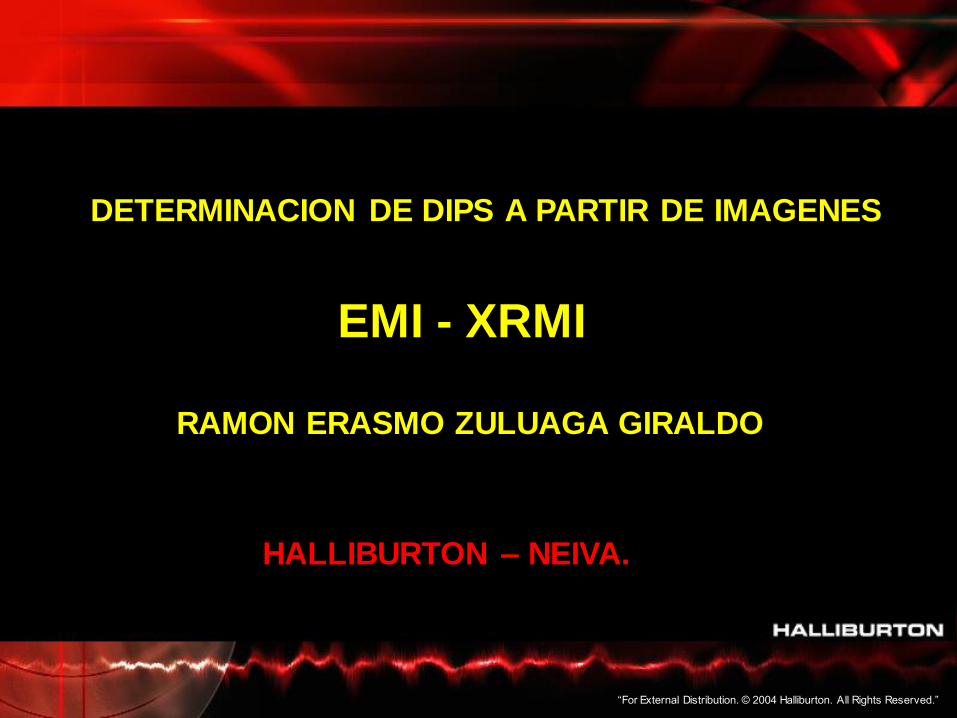
FUNDAMENTO DE LAS ONDAS DE BUZAMIENTO.

“For External Distribution. © 2004 Halliburton. All Rights Reserved.”
DETERMINACIN DEL DIP EN
POZO. – Inclinacion y
buzamiento de estratos.
EL DESPLAZAMIENTO ES LA
DISTANCIA ENTRE EL TOPE DE LA
ONDA SINOSOIDAL ( MAXIMO ) Y
EL FONDO DE LA ONDA
SINOSOIDAL ( MINIMO ).
displacement
hole diameter Dip mag = arc tan
El diámetro del pozo se deriva de las
Lecturas del caliper.
El azimut del minimo de la onda sinusoidal
Determina la dirección del Dip.

“For External Distribution. © 2004 Halliburton. All Rights Reserved.”
4 1/2”
displacement
hole diameter Dip mag = arc tan
4.5”
8” (from caliper)
Dip mag = arc tan
Dip mag = 29 degrees
Ejemplo de determinación De Dip.
• Pozo aproximadamente vertical ( según data
De navegación ).
El azimut del mínimo de la onda
Sinusoidal esta ligeramente al sur
Del oeste.

“For External Distribution. © 2004 Halliburton. All Rights Reserved.”
DEFINICIONES.
Dip aparente.
Referenciado al norte magnético y plano de los electrodos de la
Herramienta, es igual al dip del plano del estrato relativo al pozo.
Dip verdadero.
Referenciado al norte verdadero y al plano horizontal.
“For External Distribution. © 2004 Halliburton. All Rights Reserved.”
DEFINICIONES.
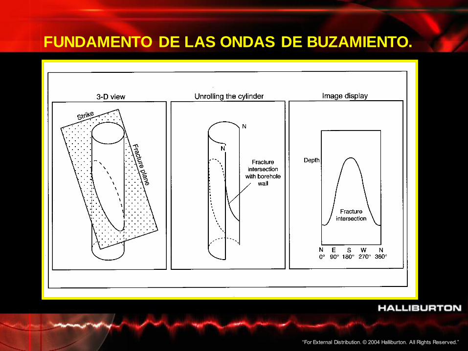
Azimut. – distancia del ángulo
Horizontal desde una dirección
De referencia fijo hasta una
posición particular.
Dip. – Cantidad con una Magnitud y dirección.
Dip angle. – Angulo entre el
Plano horizontal y el plano de
Inclinación. “ bedding plane ”.
Dip azimut. – Dirección entre el Plano inclinado con respecto al
Norte. “ bedding plane ”.

“For External Distribution. © 2004 Halliburton. All Rights Reserved.”
DEFINICIONES.
Drift angle – ángulo de
Desviación del pozo respecto a
La vertical.
Drift azimut – dirección de
la desviación del pozo Respecto al norte
Inclinación – grado de
Desviación con respecto a la
Horizontal o la vertical.
Declinación magnética – valor, En grados, que el norte
Magnético difiere del norte
Real para una locación
especifica.

“For External Distribution. © 2004 Halliburton. All Rights Reserved.”
DEFINICIONES.
Regional dip – inclinación de los
Sedimentos cuando la dirección
Promedia es constante sobre un
Área amplia.
Dip estratigráfico – se refiere a La orientación de un estrato al
Momento de la deposición.
Dip estructural – inclinación de
Sedimentos aparte de altas áreas
sub. superficiales.
-inclination of sediments away
From local sub - surface high area.
“For External Distribution. © 2004 Halliburton. All Rights Reserved.”
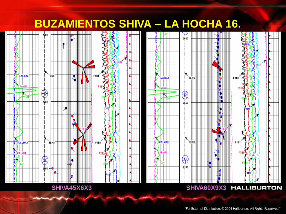
BUZAMIENTOS SHIVA – LA HOCHA 16.
SHIVA45X6X3 SHIVA60X9X3
“For External Distribution. © 2004 Halliburton. All Rights Reserved.”
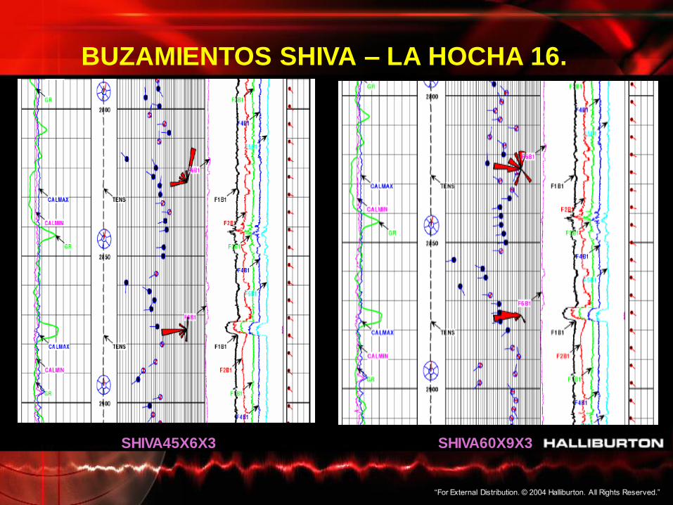
BUZAMIENTOS SHIVA – LA HOCHA 16.
SHIVA45X6X3 SHIVA60X9X3
“For External Distribution. © 2004 Halliburton. All Rights Reserved.”
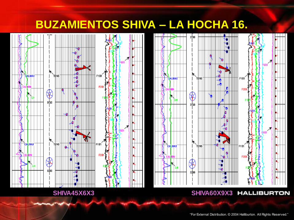
BUZAMIENTOS SHIVA – LA HOCHA 16.
SHIVA45X6X3 SHIVA60X9X3
“For External Distribution. © 2004 Halliburton. All Rights Reserved.”
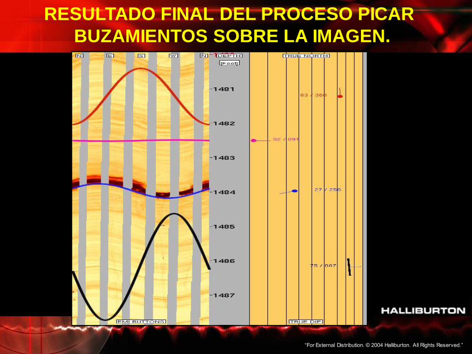
RESULTADO FINAL DEL PROCESO PICAR
BUZAMIENTOS SOBRE LA IMAGEN.
“For External Distribution. © 2004 Halliburton. All Rights Reserved.”
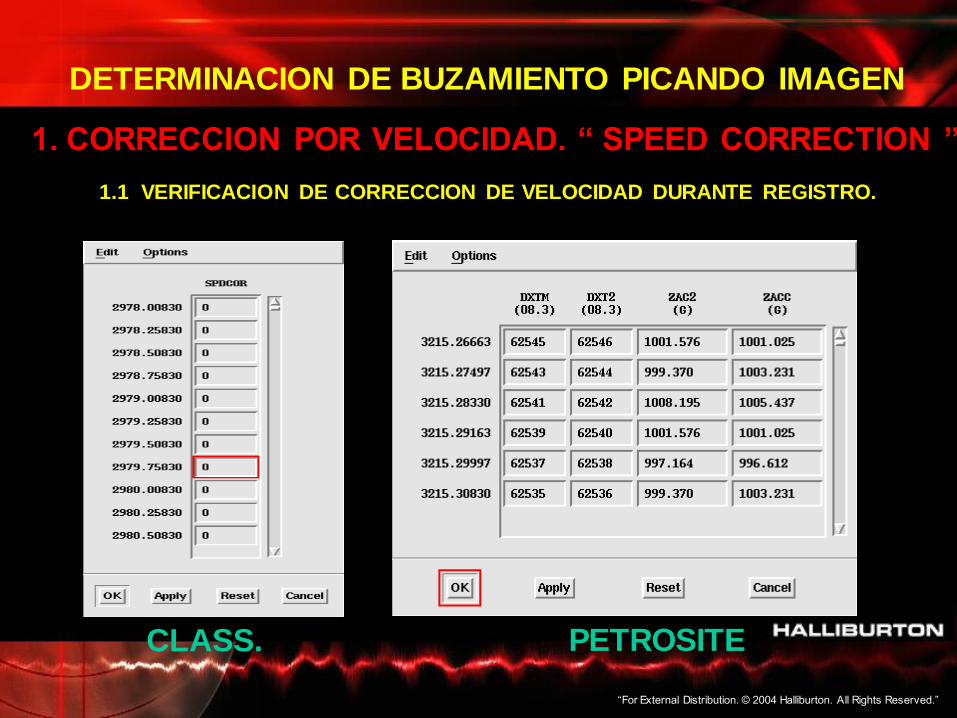
DETERMINACION DE BUZAMIENTO PICANDO IMAGEN
1. CORRECCION POR VELOCIDAD. “ SPEED CORRECTION ”
CLASS. PETROSITE
1.1 VERIFICACION DE CORRECCION DE VELOCIDAD DURANTE REGISTRO.
“For External Distribution. © 2004 Halliburton. All Rights Reserved.”
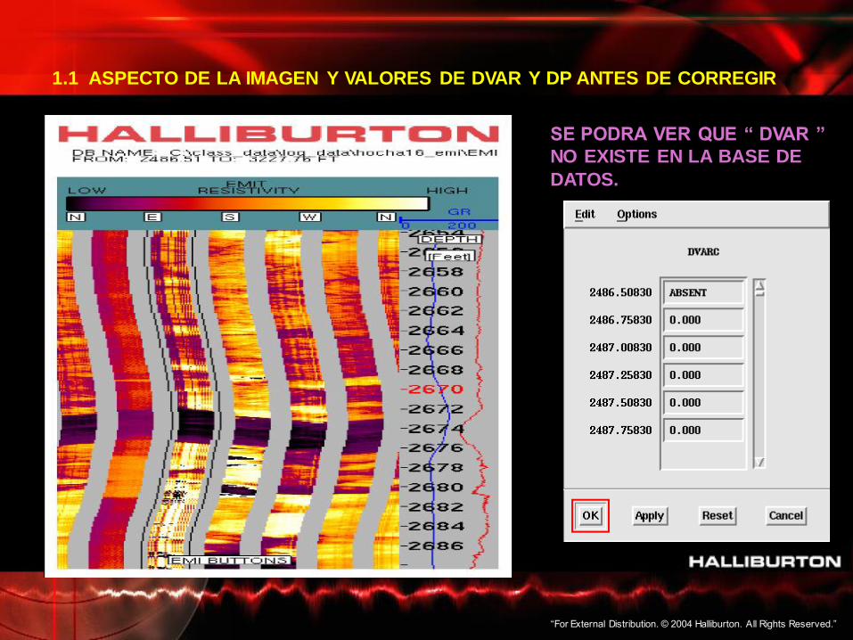
1.1 ASPECTO DE LA IMAGEN Y VALORES DE DVAR Y DP ANTES DE CORREGIR
SE PODRA VER QUE “ DVAR ”
NO EXISTE EN LA BASE DE
DATOS.
“For External Distribution. © 2004 Halliburton. All Rights Reserved.”
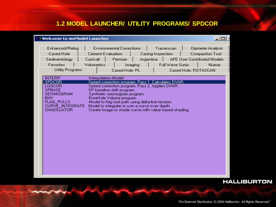
1.2 MODEL LAUNCHER/ UTILITY PROGRAMS/ SPDCOR
“For External Distribution. © 2004 Halliburton. All Rights Reserved.”
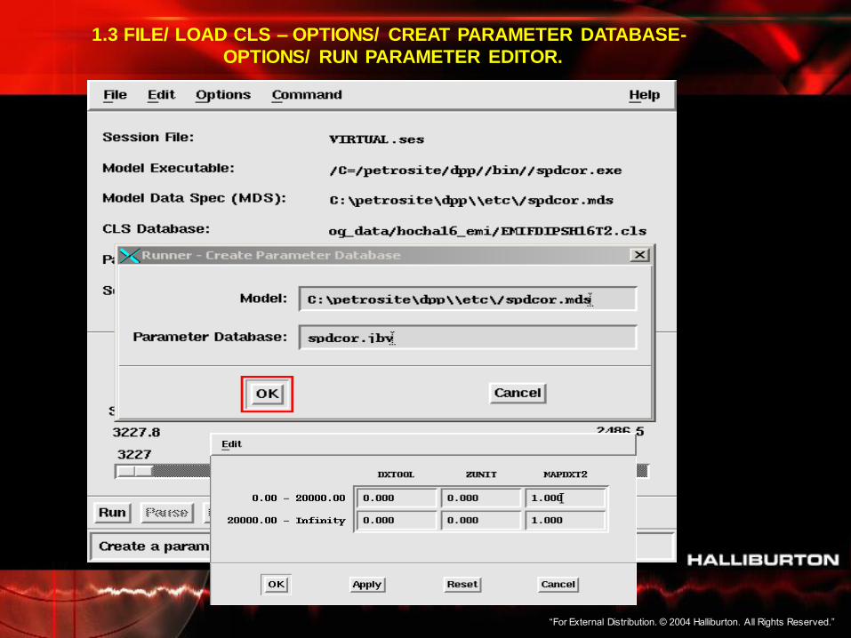
1.3 FILE/ LOAD CLS – OPTIONS/ CREAT PARAMETER DATABASE-
OPTIONS/ RUN PARAMETER EDITOR.
“For External Distribution. © 2004 Halliburton. All Rights Reserved.”
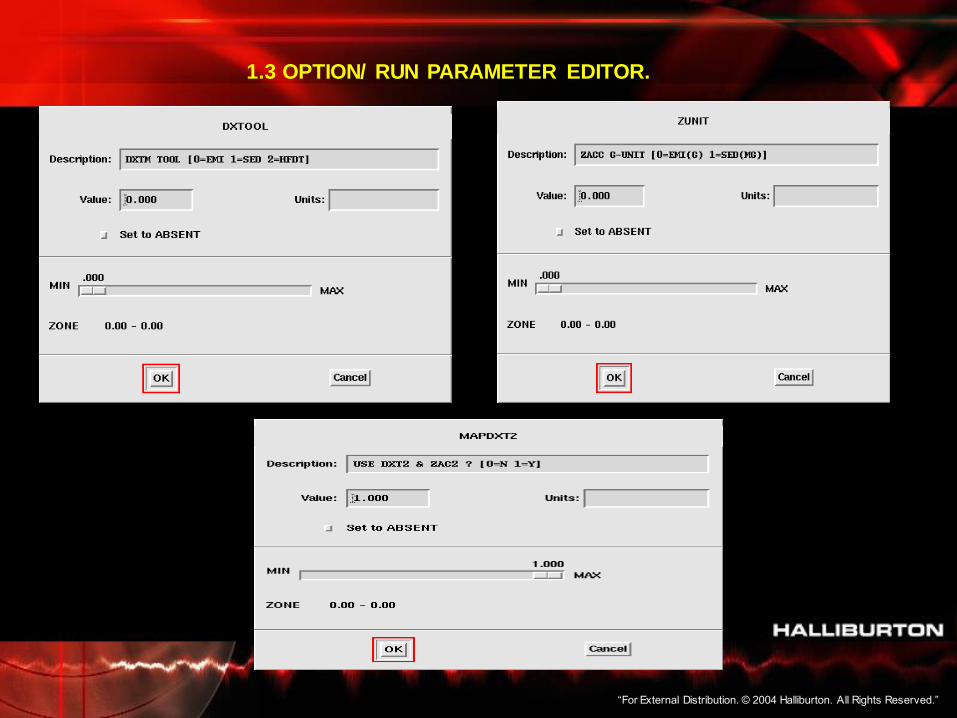
1.3 OPTION/ RUN PARAMETER EDITOR.
“For External Distribution. © 2004 Halliburton. All Rights Reserved.”
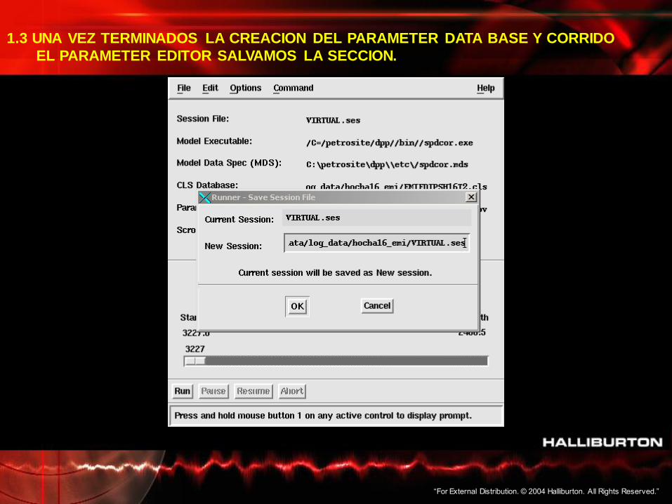
1.3 UNA VEZ TERMINADOS LA CREACION DEL PARAMETER DATA BASE Y CORRIDO
EL PARAMETER EDITOR SALVAMOS LA SECCION.
“For External Distribution. © 2004 Halliburton. All Rights Reserved.”
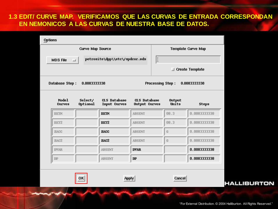
1.3 EDIT/ CURVE MAP. VERIFICAMOS QUE LAS CURVAS DE ENTRADA CORRESPONDAN
EN NEMONICOS A LAS CURVAS DE NUESTRA BASE DE DATOS.
“For External Distribution. © 2004 Halliburton. All Rights Reserved.”
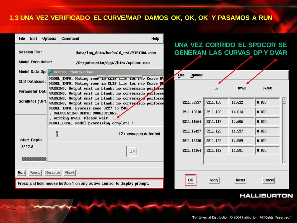
1.3 UNA VEZ VERIFICADO EL CURVE/MAP DAMOS OK, OK, OK Y PASAMOS A RUN
UNA VEZ CORRIDO EL SPDCOR SE
GENERAN LAS CURVAS DP Y DVAR
“For External Distribution. © 2004 Halliburton. All Rights Reserved.”
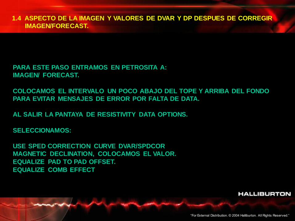
1.4 ASPECTO DE LA IMAGEN Y VALORES DE DVAR Y DP DESPUES DE CORREGIR
IMAGEN/FORECAST.
PARA ESTE PASO ENTRAMOS EN PETROSITA A:
IMAGEN/ FORECAST.
COLOCAMOS EL INTERVALO UN POCO ABAJO DEL TOPE Y ARRIBA DEL FONDO
PARA EVITAR MENSAJES DE ERROR POR FALTA DE DATA.
AL SALIR LA PANTAYA DE RESISTIVITY DATA OPTIONS.
SELECCIONAMOS:
USE SPED CORRECTION CURVE DVAR/SPDCOR
MAGNETIC DECLINATION, COLOCAMOS EL VALOR.
EQUALIZE PAD TO PAD OFFSET.
EQUALIZE COMB EFFECT.
“For External Distribution. © 2004 Halliburton. All Rights Reserved.”
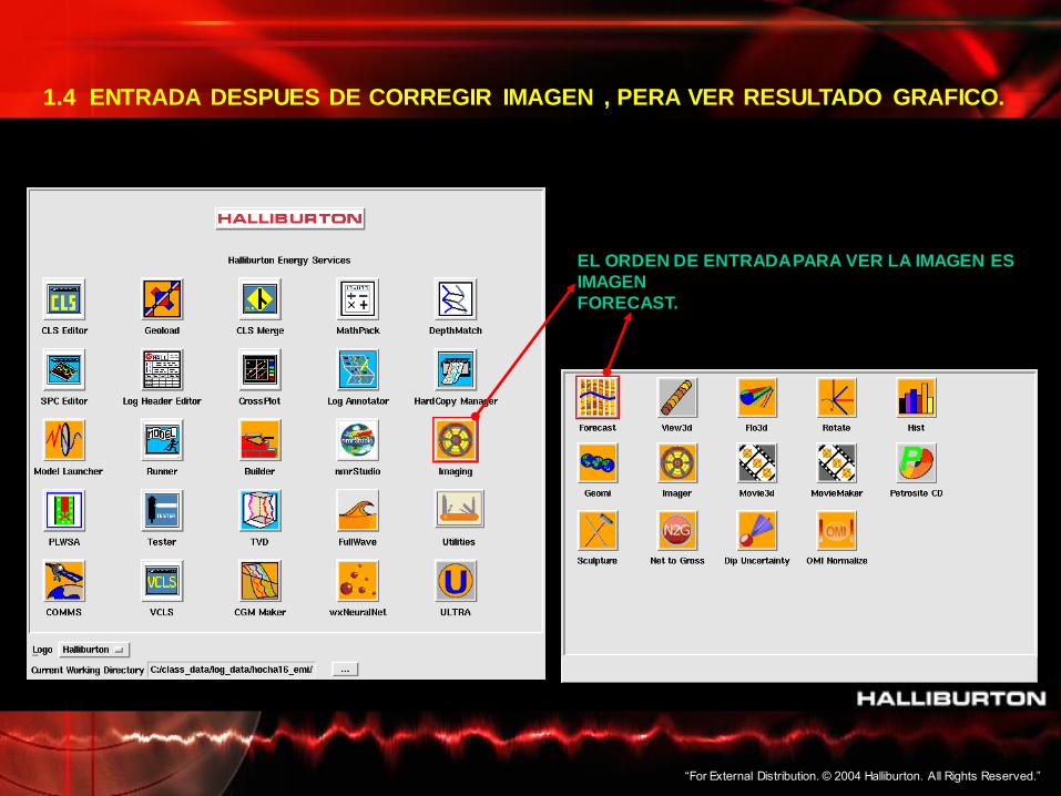
EL ORDEN DE ENTRADA PARA VER LA IMAGEN ES
IMAGEN
FORECAST.
1.4 ENTRADA DESPUES DE CORREGIR IMAGEN , PERA VER RESULTADO GRAFICO.
“For External Distribution. © 2004 Halliburton. All Rights Reserved.”
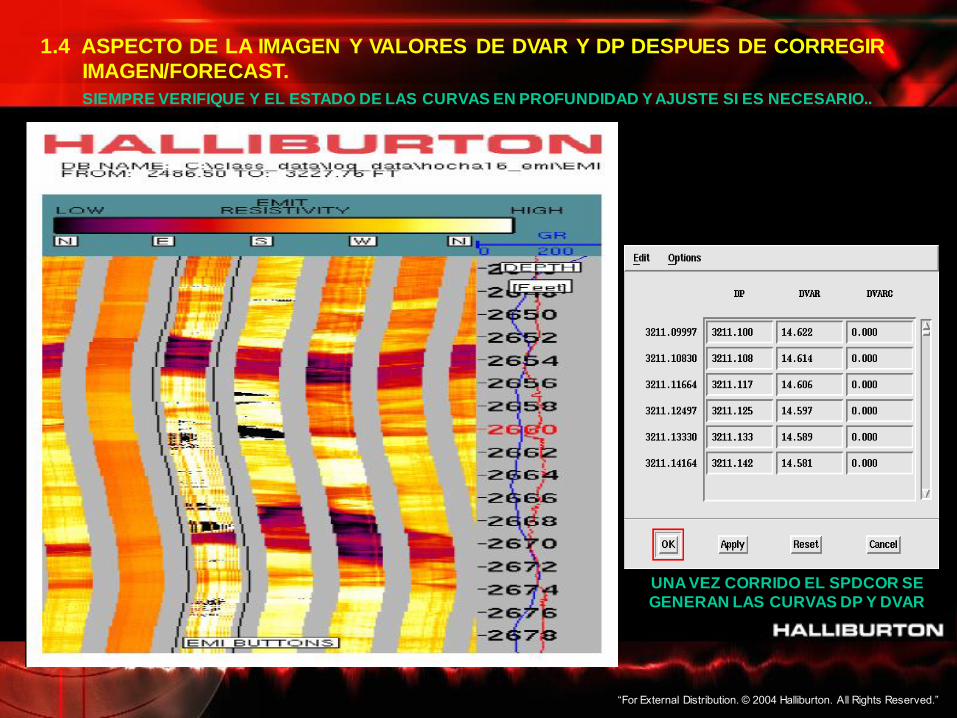
1.4 ASPECTO DE LA IMAGEN Y VALORES DE DVAR Y DP DESPUES DE CORREGIR
IMAGEN/FORECAST.
SIEMPRE VERIFIQUE Y EL ESTADO DE LAS CURVAS EN PROFUNDIDAD Y AJUSTE SI ES NECESARIO..
UNA VEZ CORRIDO EL SPDCOR SE
GENERAN LAS CURVAS DP Y DVAR
“For External Distribution. © 2004 Halliburton. All Rights Reserved.”
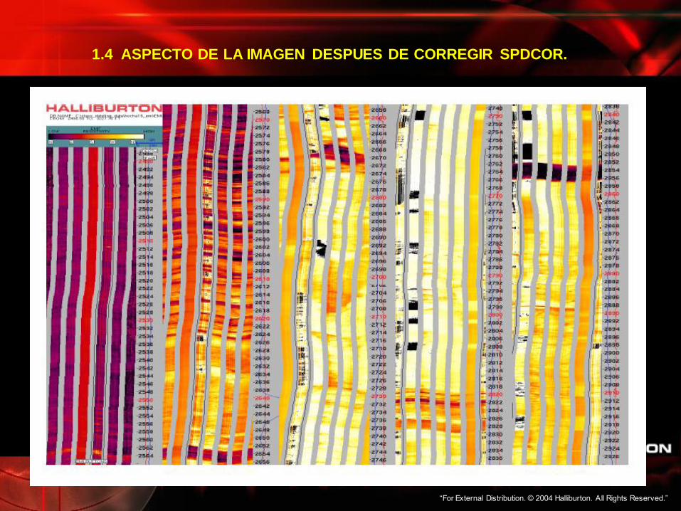
1.4 ASPECTO DE LA IMAGEN DESPUES DE CORREGIR SPDCOR.
“For External Distribution. © 2004 Halliburton. All Rights Reserved.”
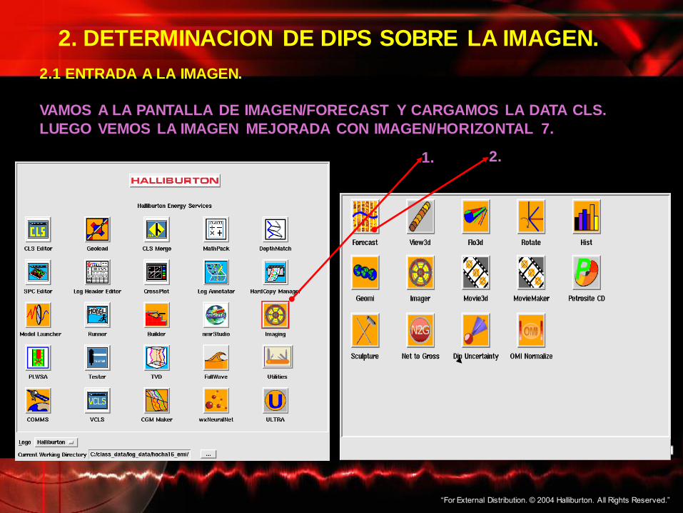
2. DETERMINACION DE DIPS SOBRE LA IMAGEN.
2.1 ENTRADA A LA IMAGEN.
VAMOS A LA PANTALLA DE IMAGEN/FORECAST Y CARGAMOS LA DATA CLS.
LUEGO VEMOS LA IMAGEN MEJORADA CON IMAGEN/HORIZONTAL 7.
1. 2.
“For External Distribution. © 2004 Halliburton. All Rights Reserved.”
VAMOS A LA PANTALLA DE IMAGEN/FORECAST Y CARGAMOS LA DATA CLS.
LUEGO VEMOS LA IMAGEN MEJORADA CON IMAGEN/HORIZONTAL 7.
APARECE LA PANTALLA DE RESISTIVITY DATA OPTIONS, SELECCIONAMOS:
USE SPEED CORRECTION CURVE DVAR/SPDCOR
DAMOS EL VALOR DE DECLINACION MAGNETICA.
EQUALIZE PAD TO PAD OFFSET.
EQUALIZE COM OFFECTT
2.2. VALORES DE LA PANTALLA DE RESISTIVIDAD

“For External Distribution. © 2004 Halliburton. All Rights Reserved.”
ASPECTO DE LA IMAGEN CARGADA POR EL PETROSITE , IMAGEN EN LA CUAL
SE GENERARAN LOS DIPS.
“For External Distribution. © 2004 Halliburton. All Rights Reserved.”
DAMOS CLICK CON EL RATON DERECHO Y GENERAMOS LA ONDA SENOSOIDAL
QUE CORRESPONDA A LA IMAGEN.
UNA VEZ GENERADA LA ONDA DAMOS UN NUMERO DE 1 A 5, SEGÚN LA ONDA
CUBRA O NO TODOS LOS PATINES.
1 ES TOTALMENTE SEGUROS DE TAL BUZAMIENTO Y 5 ES TOTALMENTE
INSEGUROS.
2.3 GENERACION DEL DIP MANUAL.
“For External Distribution. © 2004 Halliburton. All Rights Reserved.”
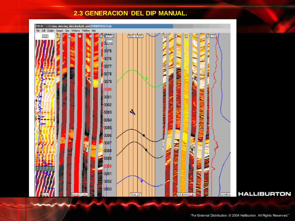
2.3 GENERACION DEL DIP MANUAL.
“For External Distribution. © 2004 Halliburton. All Rights Reserved.”
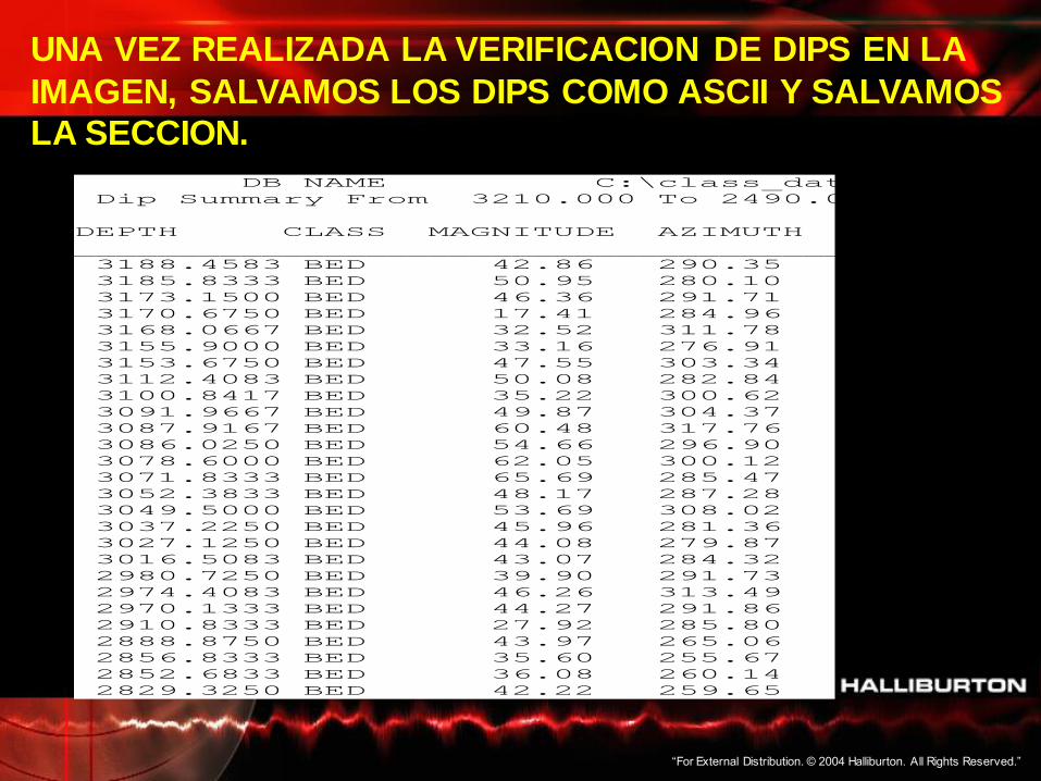
DB NAME C:\class_data\log_data\hocha16_emi\EMIFDIPSH16T2.cls
Dip Summary From 3210.000 To 2490.000 F
DEPTH CLASS MAGNITUDE AZIMUTH QUALITY CONF TYPE PATTERN DIPTYPE
_____________________________________________________________________________
3188.4583 BED 42.86 290.35 3.00 12.48 F Cross Bedding
3185.8333 BED 50.95 280.10 2.00 12.51 G Bed Boundary
3173.1500 BED 46.36 291.71 3.00 12.53 F Cross Bedding
3170.6750 BED 17.41 284.96 1.00 13.29 E BEDDING
3168.0667 BED 32.52 311.78 3.00 13.16 F Cross Bedding
3155.9000 BED 33.16 276.91 3.00 12.28 F Cross Bedding
3153.6750 BED 47.55 303.34 1.00 12.23 E BEDDING
3112.4083 BED 50.08 282.84 3.00 12.26 F Cross Bedding
3100.8417 BED 35.22 300.62 3.00 12.36 F Cross Bedding
3091.9667 BED 49.87 304.37 3.00 12.70 F Cross Bedding
3087.9167 BED 60.48 317.76 1.00 12.73 E Bed Boundary
3086.0250 BED 54.66 296.90 1.00 12.40 E Bed Boundary
3078.6000 BED 62.05 300.12 1.00 12.86 E BEDDING
3071.8333 BED 65.69 285.47 3.00 12.83 F Cross Bedding
3052.3833 BED 48.17 287.28 1.00 12.52 E Bed Boundary
3049.5000 BED 53.69 308.02 3.00 12.31 F Cross Bedding
3037.2250 BED 45.96 281.36 3.00 12.70 F Cross Bedding
3027.1250 BED 44.08 279.87 3.00 12.86 F Cross Bedding
3016.5083 BED 43.07 284.32 1.00 12.54 E Bed Boundary
2980.7250 BED 39.90 291.73 3.00 12.31 F Cross Bedding
2974.4083 BED 46.26 313.49 3.00 12.47 F Cross Bedding
2970.1333 BED 44.27 291.86 4.00 12.49 P Cross Bedding
2910.8333 BED 27.92 285.80 3.00 12.54 F Cross Bedding
2888.8750 BED 43.97 265.06 3.00 12.30 F Cross Bedding
2856.8333 BED 35.60 255.67 1.00 12.35 E BEDDING
2852.6833 BED 36.08 260.14 1.00 12.38 E BEDDING
2829.3250 BED 42.22 259.65 1.00 12.35 E BEDDING
UNA VEZ REALIZADA LA VERIFICACION DE DIPS EN LA
IMAGEN, SALVAMOS LOS DIPS COMO ASCII Y SALVAMOS
LA SECCION.
“For External Distribution. © 2004 Halliburton. All Rights Reserved.”
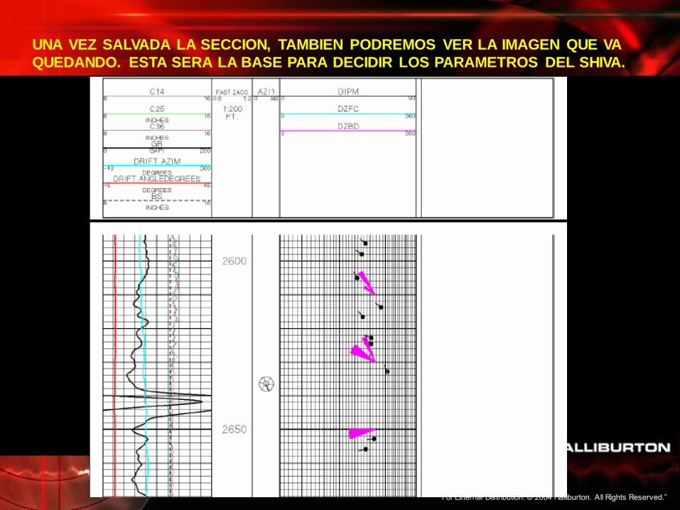
UNA VEZ SALVADA LA SECCION, TAMBIEN PODREMOS VER LA IMAGEN QUE VA
QUEDANDO. ESTA SERA LA BASE PARA DECIDIR LOS PARAMETROS DEL SHIVA.

“For External Distribution. © 2004 Halliburton. All Rights Reserved.”
3. GENERANDO EL TADPODE ( DESVIACION Y BUZAMIENTO DEL POZO ).
PARA ACCEDER A ESTA PANTALLA
VAMOS A MODEL LUNCHER/
PERMIAN/TADPODE
UNA VEZ EN ELLA CARGAMOS LA
BASE DE DATOS Y CREAMOS EL
PARAMETER DATA BASE.
DAMOS OK. ESPERAMOS QUE
TERMINE EL PROCESO Y
SALVAMOS LA SECCION.
“For External Distribution. © 2004 Halliburton. All Rights Reserved.”
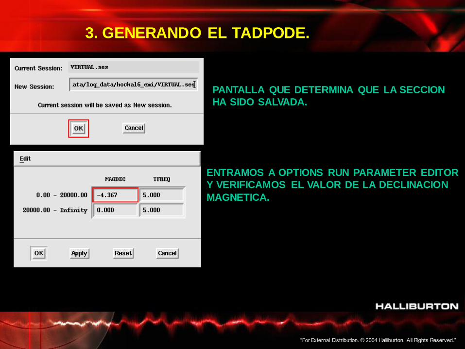
3. GENERANDO EL TADPODE.
PANTALLA QUE DETERMINA QUE LA SECCION
HA SIDO SALVADA.
ENTRAMOS A OPTIONS RUN PARAMETER EDITOR
Y VERIFICAMOS EL VALOR DE LA DECLINACION
MAGNETICA.
“For External Distribution. © 2004 Halliburton. All Rights Reserved.”
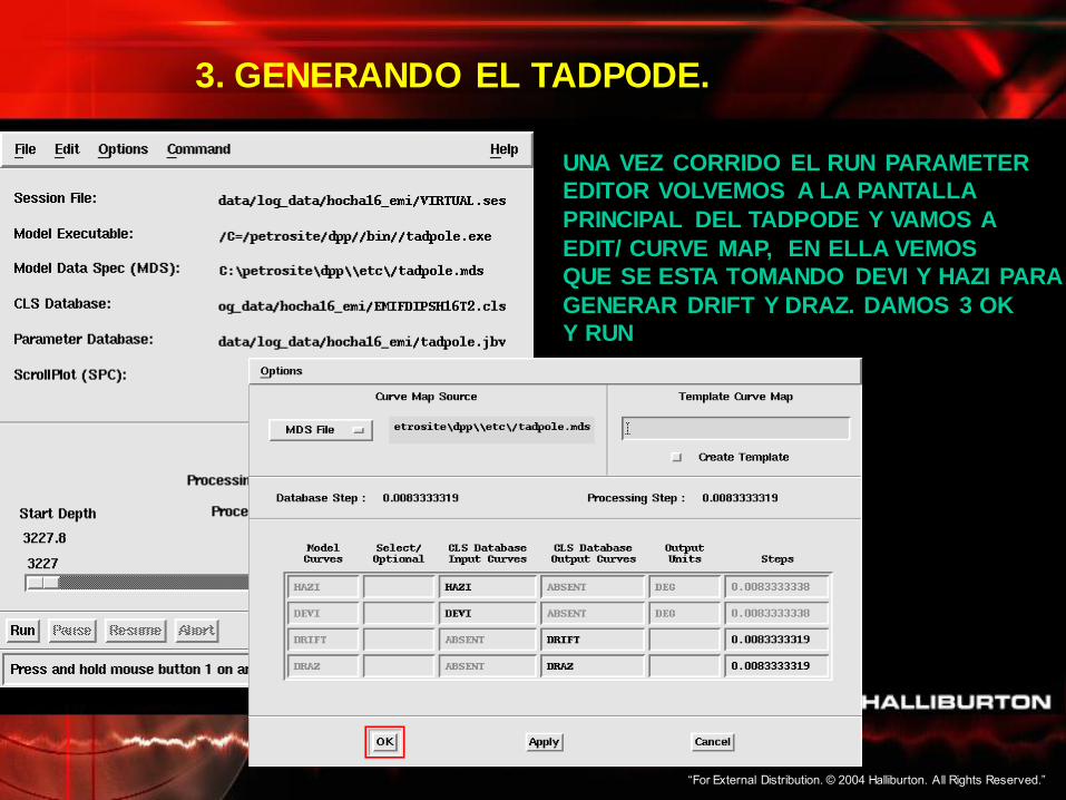
3. GENERANDO EL TADPODE.
UNA VEZ CORRIDO EL RUN PARAMETER
EDITOR VOLVEMOS A LA PANTALLA
PRINCIPAL DEL TADPODE Y VAMOS A
EDIT/ CURVE MAP, EN ELLA VEMOS
QUE SE ESTA TOMANDO DEVI Y HAZI PARA
GENERAR DRIFT Y DRAZ. DAMOS 3 OK
Y RUN
“For External Distribution. © 2004 Halliburton. All Rights Reserved.”
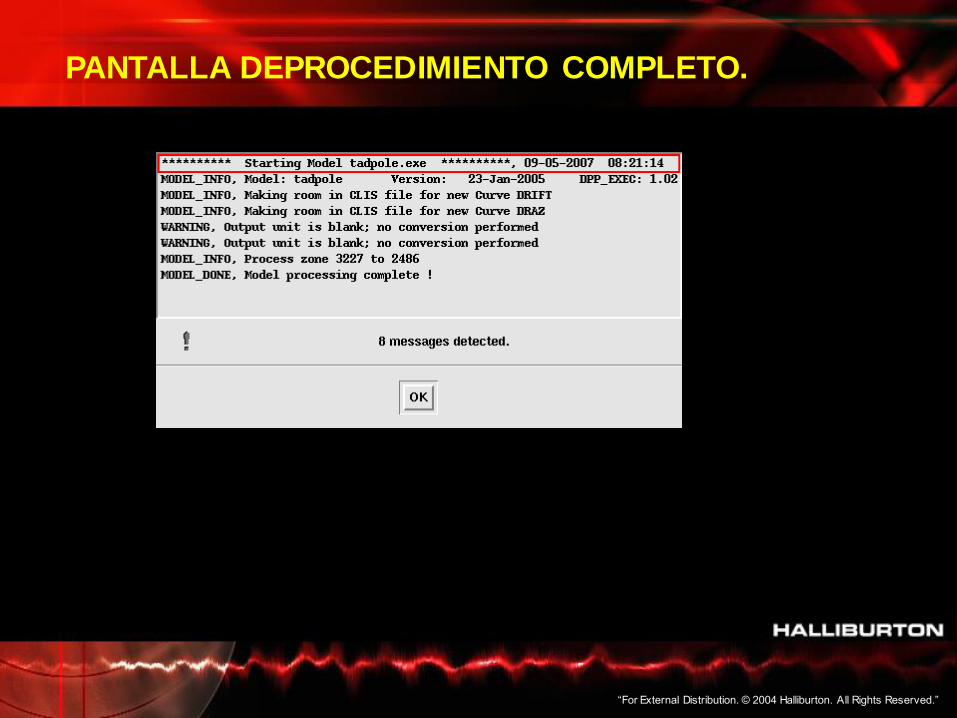
PANTALLA DEPROCEDIMIENTO COMPLETO.
“For External Distribution. © 2004 Halliburton. All Rights Reserved.”
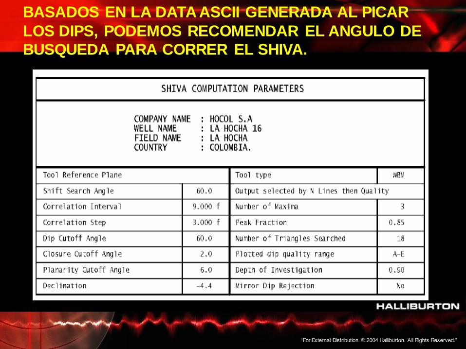
BASADOS EN LA DATA ASCII GENERADA AL PICAR
LOS DIPS, PODEMOS RECOMENDAR EL ANGULO DE
BUSQUEDA PARA CORRER EL SHIVA.
“For External Distribution. © 2004 Halliburton. All Rights Reserved.”
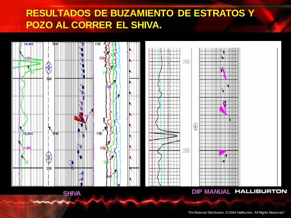
RESULTADOS DE BUZAMIENTO DE ESTRATOS Y
POZO AL CORRER EL SHIVA.
SHIVA DIP MANUAL
“For External Distribution. © 2004 Halliburton. All Rights Reserved.”
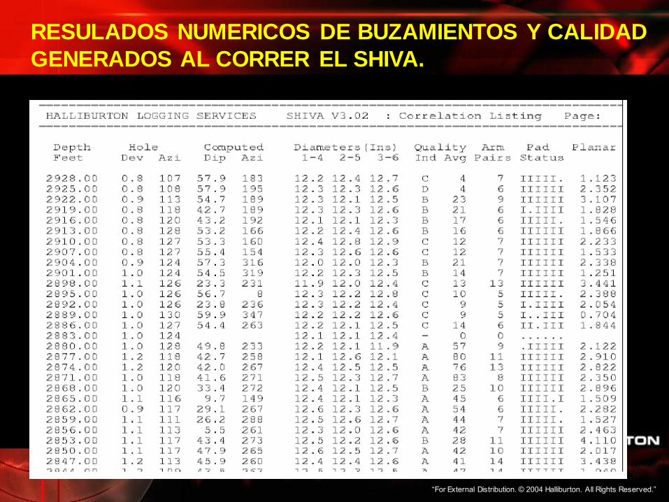
RESULADOS NUMERICOS DE BUZAMIENTOS Y CALIDAD
GENERADOS AL CORRER EL SHIVA.
“For External Distribution. © 2004 Halliburton. All Rights Reserved.”
MUCHAS GRACIAS.