DIAGRAMAS DE

EQUILIBRIO

UNIDAD 1. Fundamentos Termodinámicos

DIAGRAMAS DE EQUILIBRIO

Son representaciones de temperatura (en algunas

ocasiones presión) frente a composición

Gráficamente se resumen los intervalos de temperatura (o

presión) en los que ciertas fases, o mezclas de fases, existen

en condiciones de equilibrio termodinámico

Se puede deducir el efecto de la temperatura sobre los

sólidos y las reacciones que pueden producirse entre sólidos

Se aplican en condiciones de equilibrio termodinámico, en

la práctica son muy útiles en condiciones de no equilibrio

History

In 1876 and 1878 J.Willard Gibbs published work that provides

the thermodynamic basis for understanding the equilibrium

state of any arbitrary combination of substances under

specified conditions.

However, Gibbs had been in communication with James

Clerk Maxwell, and Maxwell knew of and understood Gibbs’

work.

Though Maxwell died only a very few years after the

publication of Gibbs’work, Maxwell had made known the

work to Van der Waals who in turn made it known to H.W.

Bakhuis Roozeboom.

Bakhuis Roozeboom successfully incorporated Gibbs’

concepts into his own work.

What is believed to be the first temperature-

composition plot was made by Roberts-Austen and

was published in 1875, the Ag–Cu system.

The system needs a thermocouple instead of ordinary

thermometer. Improvement awaited the

development of a stable thermocouple, and a

reliable Pt–Pt10%Rh thermocouple was developed by

Le Chatelier in 1877.

Sorby was contemporaneous with Roberts-Austen

and he named the phases which he observed in

his metallographic studies of iron–carbon alloys

as follows:

Ferrite for the terminal BCC-Fe solution;

austenite for the FCC-Fe solution;

pearlite for the Fe–Fe3C eutectic;

cementite for the Fe3C phase;

and martensite for the hardening precipitate

phase.

Sorby chose the name austenite in honor of

Roberts-Austen

1897 Roberts-Austen diagram has been called

“the first phase diagram”.

The temperature-composition diagrams of that

period were plotted from dynamic

measurements and the Roberts-Austen diagram

was not an “equilibrium” diagram since it lacked

compatibility with the equilibrium reversibility

inherent in the thermodynamic constraints

codified by Gibbs.

Roberts Austen invited Bakhuis Roozeboom to modify

the 1899 temperature composition diagram for

compatibility with the Gibbs phase rule. The result was

a thermodynamically valid equilibrium Fe–Fe3C

diagram in 1900

Many materials are used in “frozen in” non-equilibrium

states and phase diagrams provide a means of

showing where the material started and where

equilibrium will be reached, the path that the

material should follow in transforming from initial state

to equilibrium is cogent to understanding the state

where it might be in a non-equilibrium “freeze”

The Fe–C diagram without the metastable Fe3C has also

been proven useful in cast iron technology.

Sorby became aware of the Widmanstätten prints and

used an optical microscope with polished and etched

specimens to make the aforementioned study of the

microstructures of iron–carbon alloys.

Metallography, X-ray diffraction, electron and neutrón

diffraction

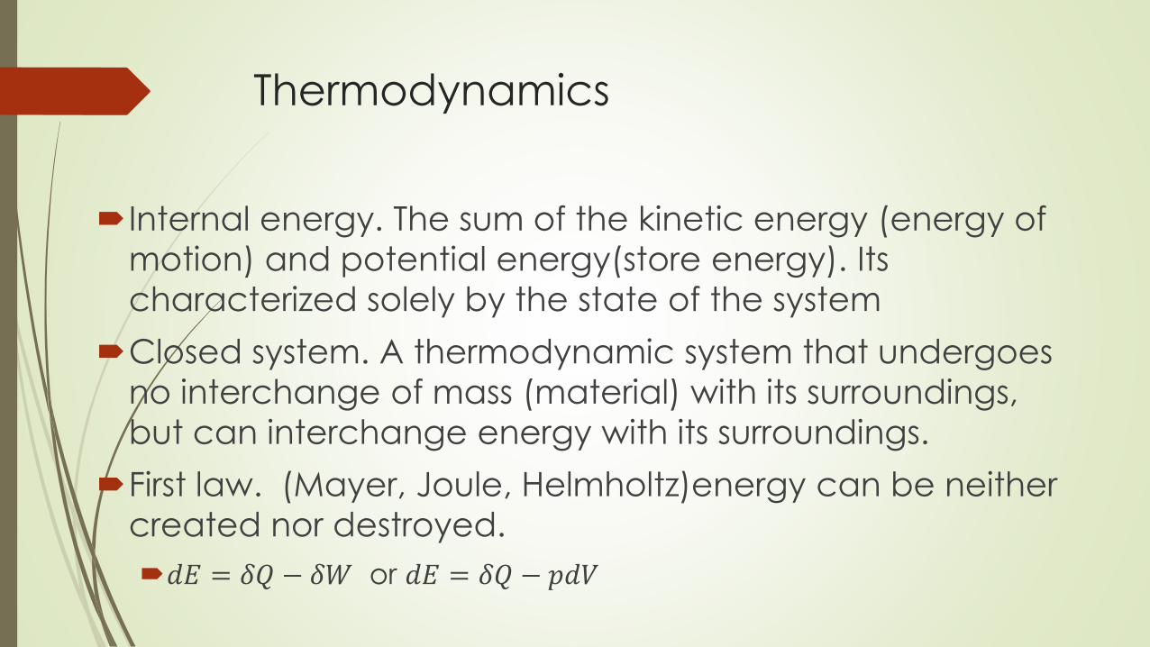
Internal energy. The sum of the kinetic energy (energy of

motion) and potential energy(store energy). Its

characterized solely by the state of the system

Closed system. A thermodynamic system that undergoes

no interchange of mass (material) with its surroundings,

but can interchange energy with its surroundings.

First law. (Mayer, Joule, Helmholtz)energy can be neither

created nor destroyed.

𝑑𝐸 = 𝛿𝑄 − 𝛿𝑊 or 𝑑𝐸 = 𝛿𝑄 − 𝑝𝑑𝑉

Thermodynamics

Enthalpy. Thermal energy changes

under constant pressure (again

neglecting any field effects)are most

conveniently expressed in terms of

the enthalpy

Its a function of the state of the

system, as is the PV

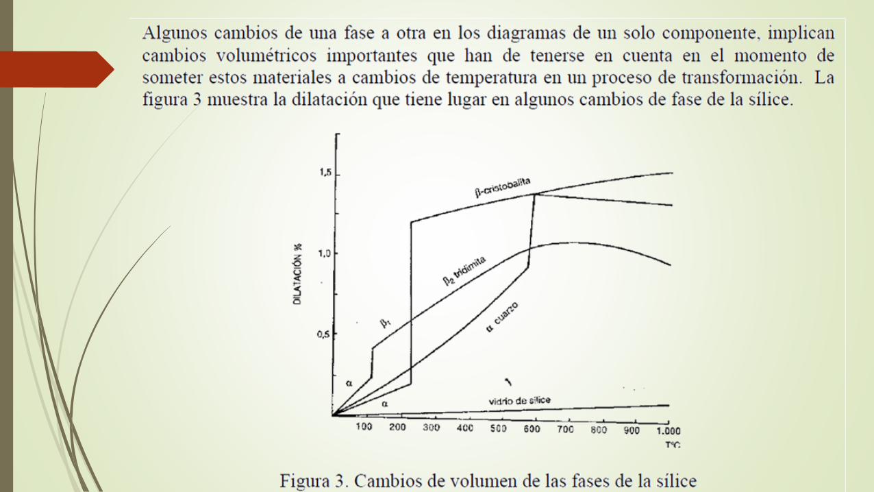
ThermodynamicsThe present treatment is meant only to highlight the factors

that need to be taken into account when constructing or

examining a phase diagram.

For any system the number of arbitrarily alterable variables

constitute the degrees of freedom, f.

For a system in which P dV work is the sole work

contribution, the first law of thermodynamics in differential

form is

dE = T dS - P dV

and T and P are system intensive variables

These two plus the number of components, c, yield the

total number of variables, n.

The number of phases, p, represent the number of ways

in which the variables are related, m. Thus the number of

degrees of freedom can be represented as

F= n – m = c – p + 2

This is the phase rule, and this in combination with

thermodynamic considerations determines the

constraints that are placed upon a phase diagram.

Along the line defining the liquid–gas equilibrium, the Gibbs

energies of the two phases must be equal, so:

ΔtG = ΔtH - TΔtS = 0

which leads to

ΔtH/T = ΔtS

At any given pressure at all temperatures below the

transition temperature, T <Tt, the liquid is the stable phase so

the Gibbs energy of the liquid must be lower than the Gibbs

energy of the gas, Gl < Gg.

Phase

Phase. Region of space occupied by a physically

homogeneous material. However, there are two uses of

the term: the strict sense normally used by physical

scientists an the somewhat looser sense normally used

by materials engineers.

In the strictest sense, homogeneous means that the

physica properties throughout the región of space

occupied by the phase are absolutely identical, and

any change in condition of state, no matter how small,

will result in a different phase.

Equilibrium

There are three types of equilibria: stable, metastable,

and unstable.

Stable equilibrium exists when the object is in its lowest

energy condition

Metastable equilibrium exists when additional energy

must be introduced before the object can reach true

stability

Unstable equilibrium exist when no additional energy is

needed before reaching metastability or stability

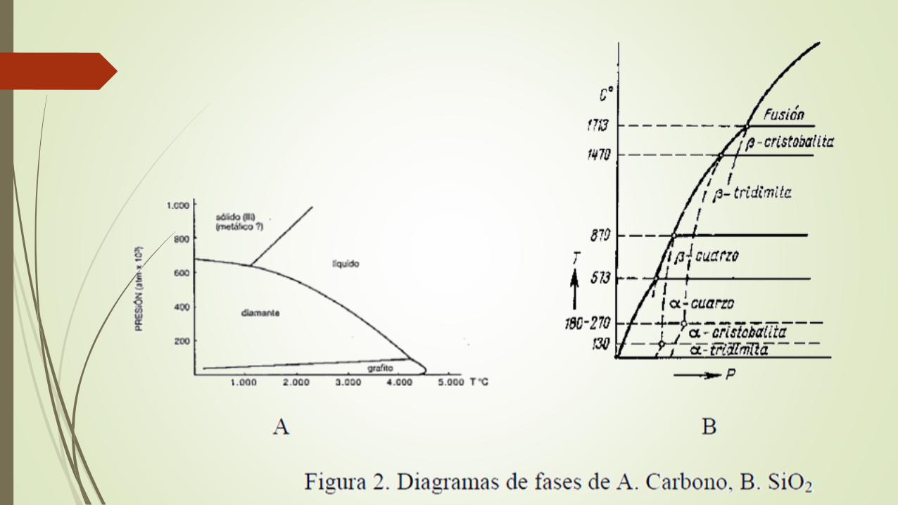
Polymorphism

The structure of solid elements and compounds under

stable equilibrium condiction is crystalline, and the cristal

structure of each is unique.

Some elements and compounds are polumorphic

(multishaped); their structure transforms from one cristal

structure to another with changes in temperatura and

pressure, each unique structure consisting a distinctively

separate phase.

Allotrpy is usually used to describe polymorphic changes

in chemical elements

Metastable phases

Under some conditions, metastable cristal

structures can form instead of stable

structures. Rapid freezing is a common

method of producing metastable

structures, but some (cementite) are

produced at moderately slow cooling

rates.

Systems

A physical system consists of a substance (or a

group of substances) that is isolated from itssurrounding (isolatedthere is no interchange of

mass between the substance and its surroundings)

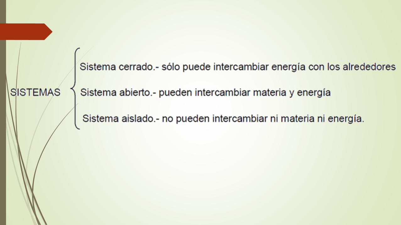
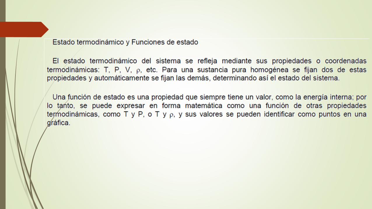
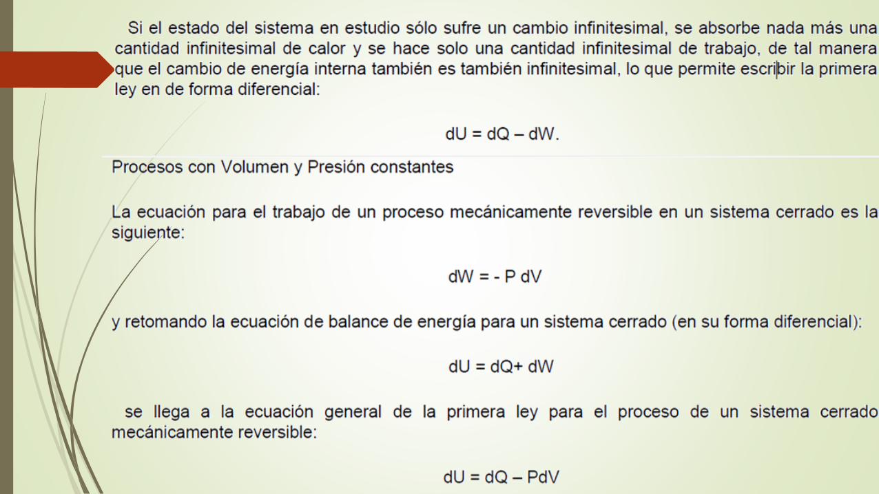
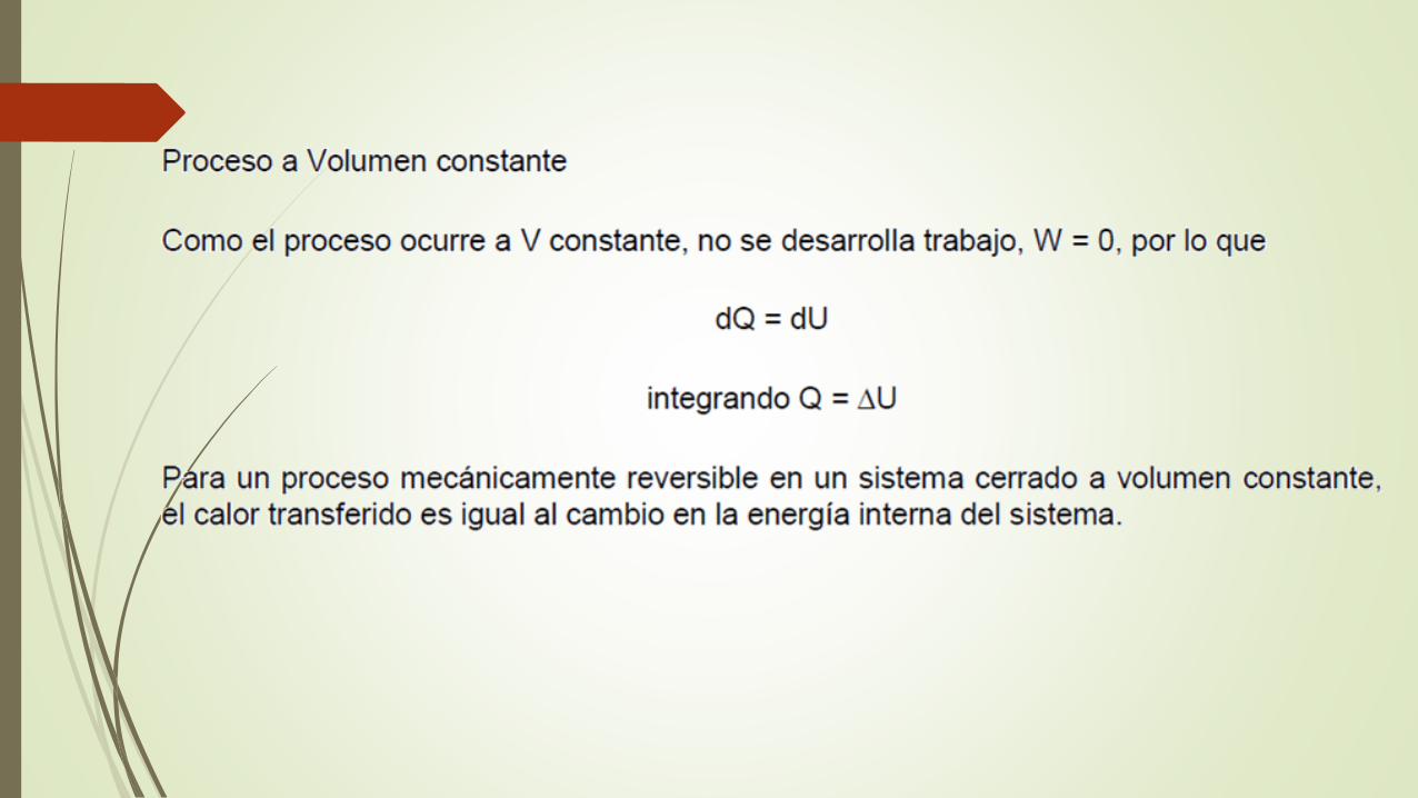
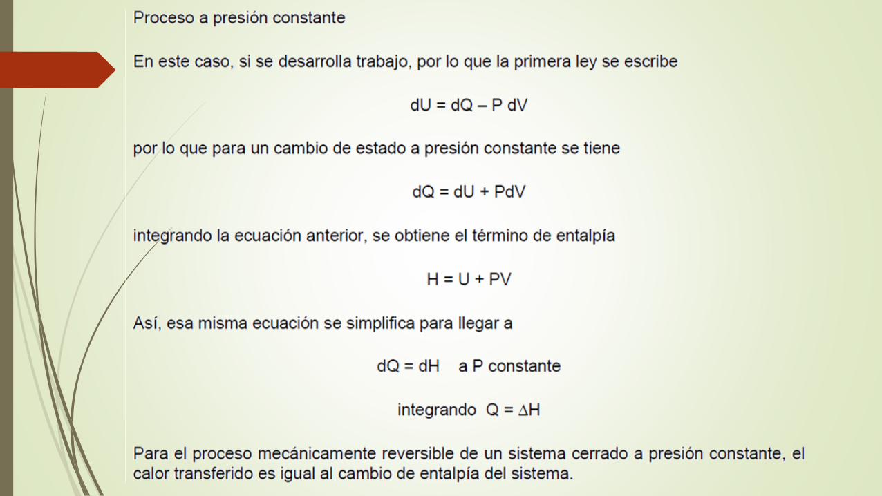
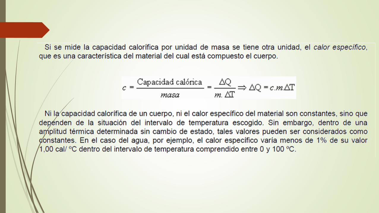
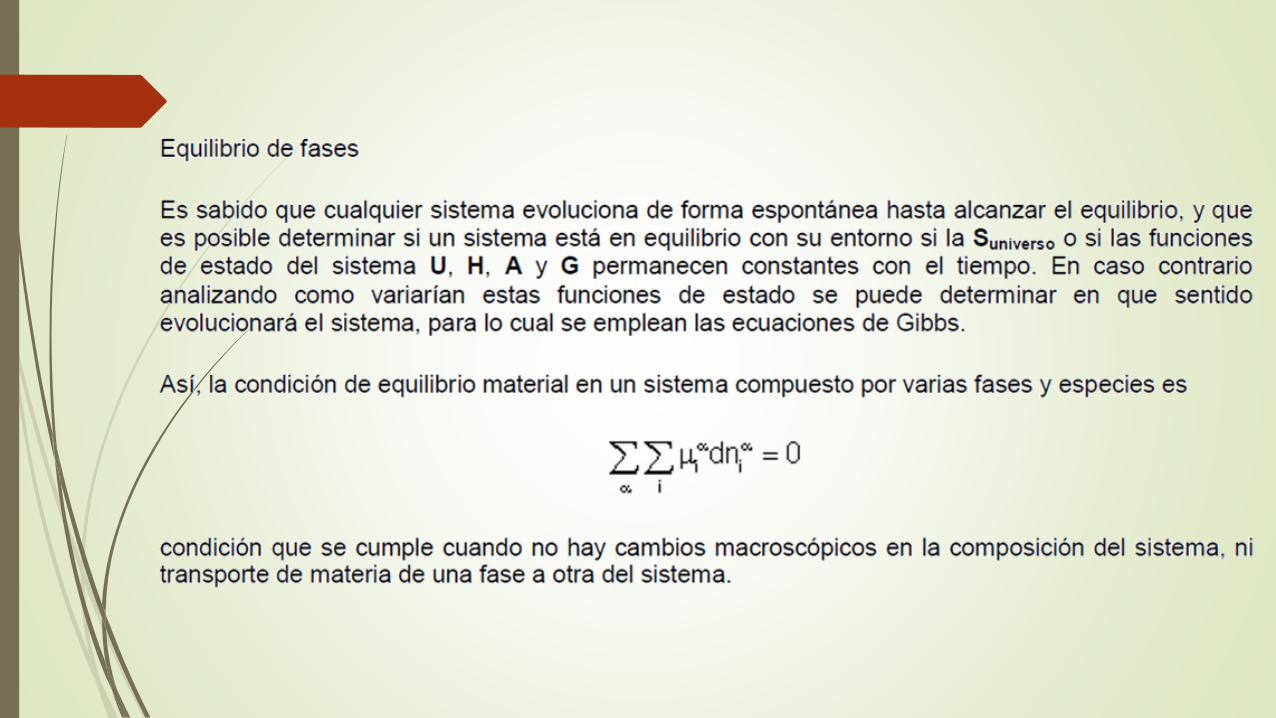
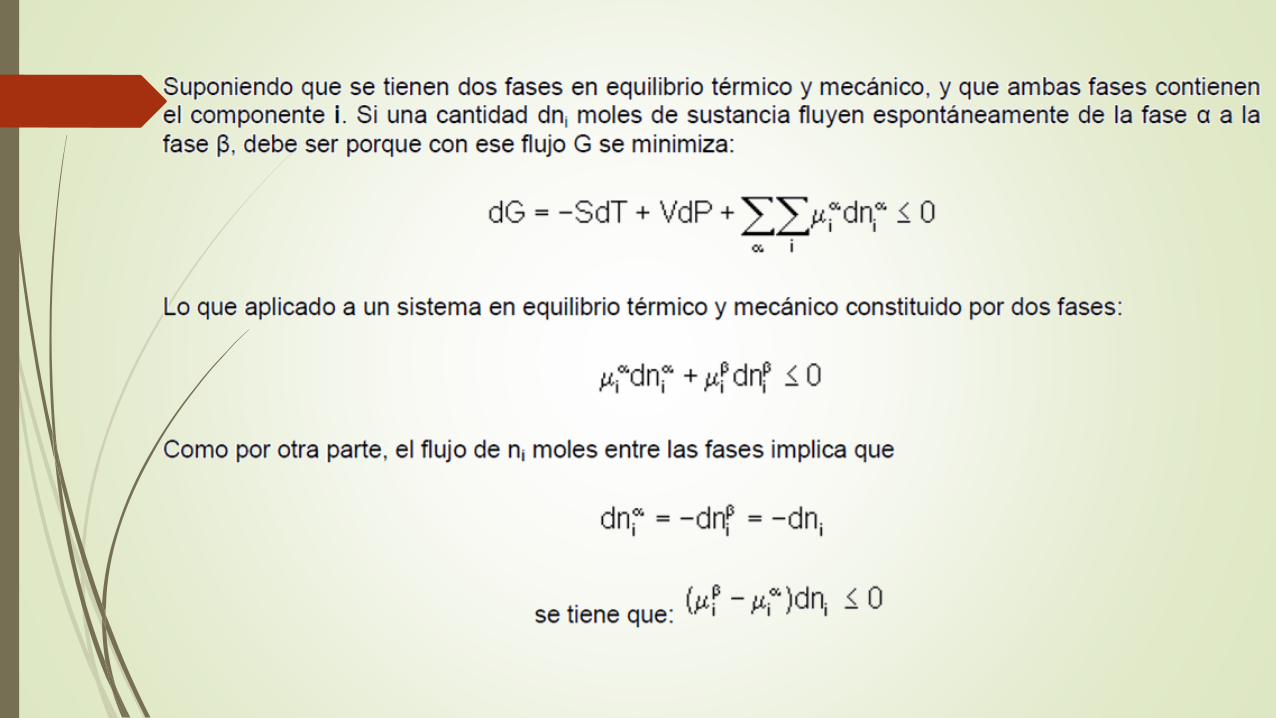
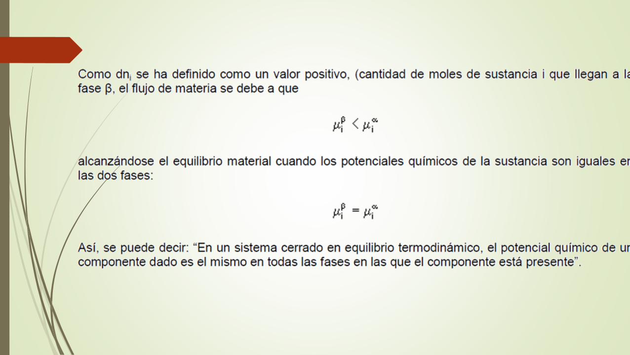
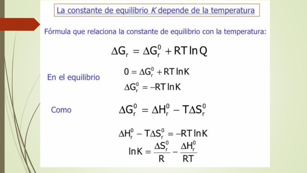
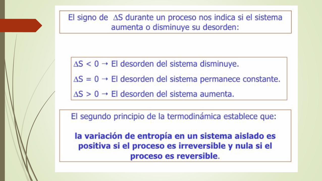
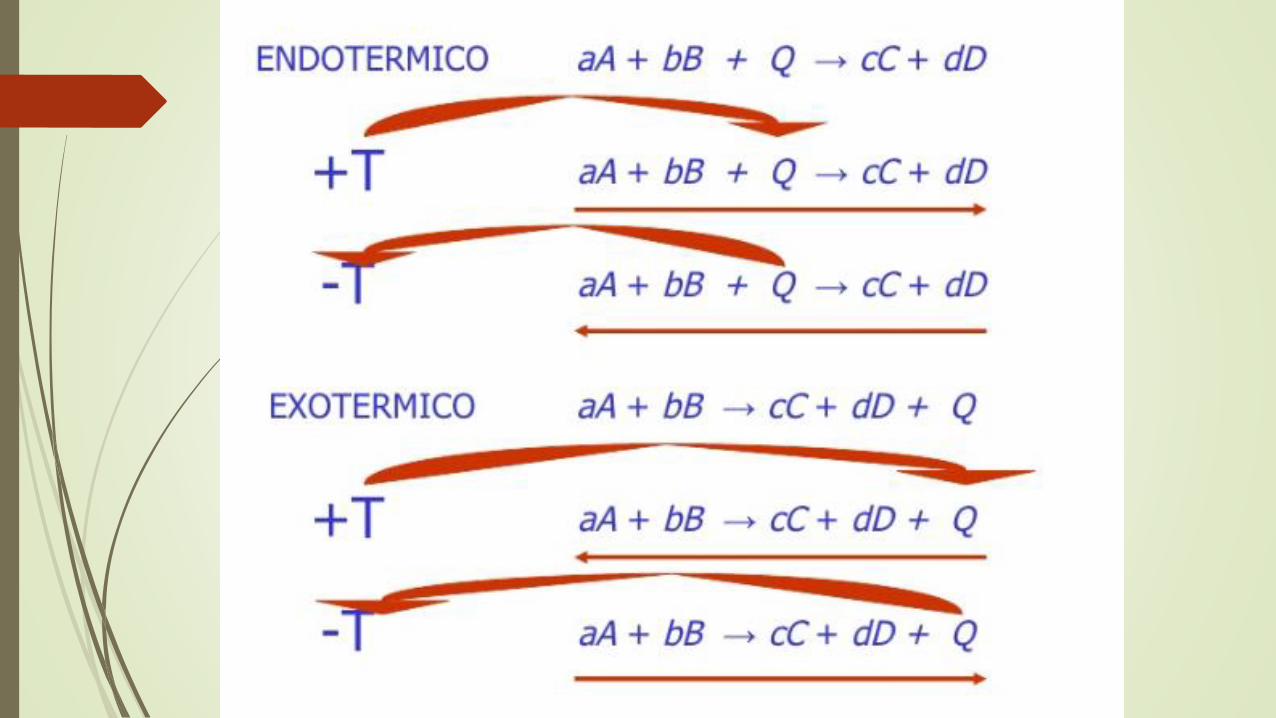
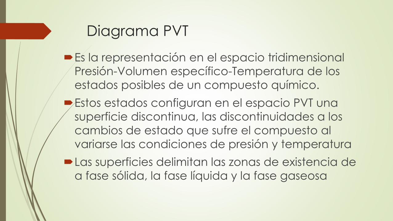
Diagrama PVT

Es la representación en el espacio tridimensional

Presión-Volumen específico-Temperatura de los

estados posibles de un compuesto químico.

Estos estados configuran en el espacio PVT una

superficie discontinua, las discontinuidades a los

cambios de estado que sufre el compuesto al

variarse las condiciones de presión y temperatura

Las superficies delimitan las zonas de existencia de

a fase sólida, la fase líquida y la fase gaseosa

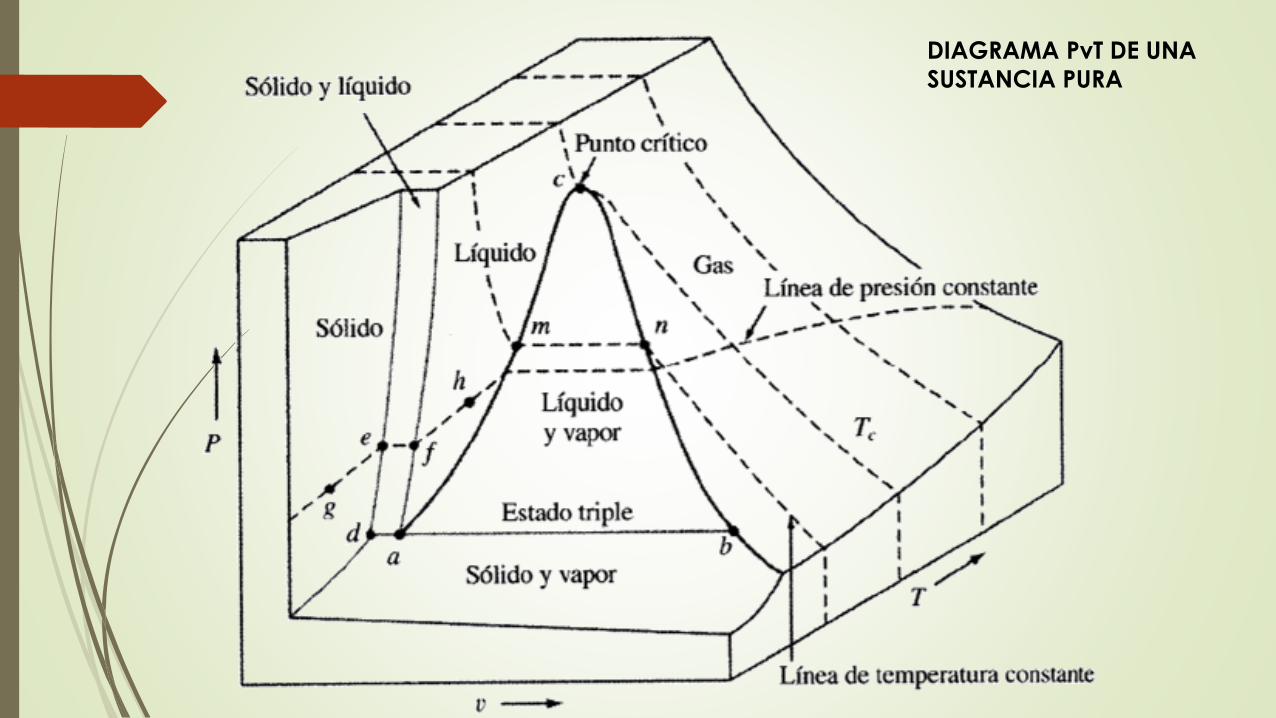
DIAGRAMA PvT DE UNA

SUSTANCIA PURA

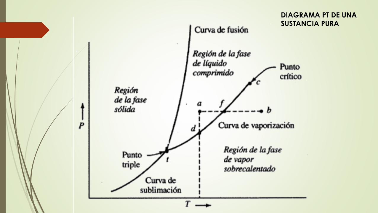
DIAGRAMA PT DE UNA

SUSTANCIA PURA

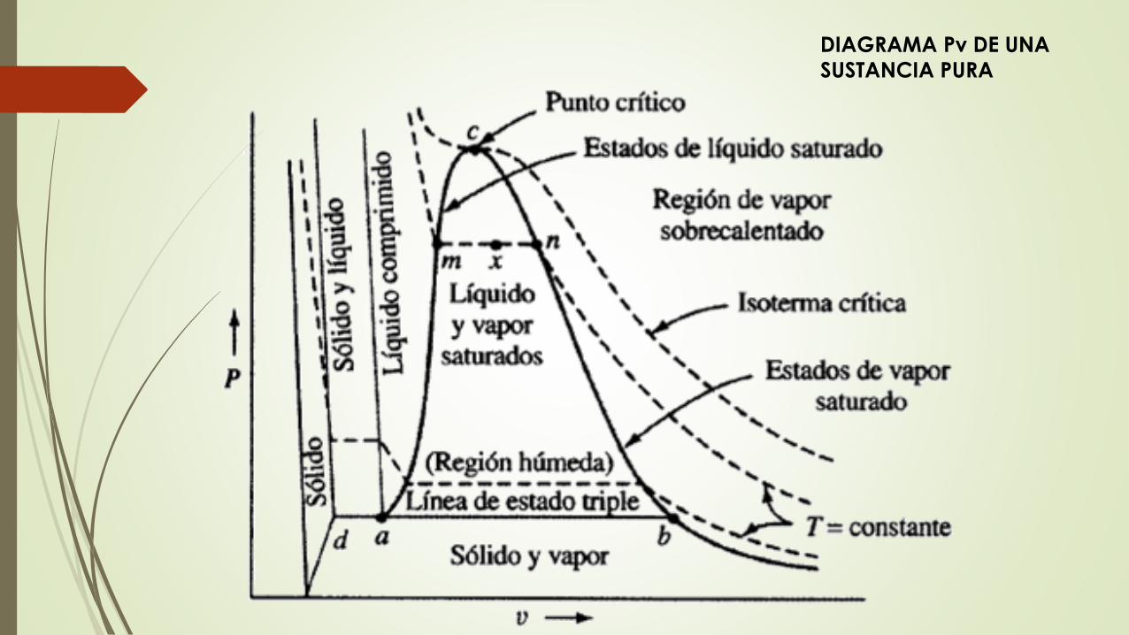
DIAGRAMA Pv DE UNA

SUSTANCIA PURA

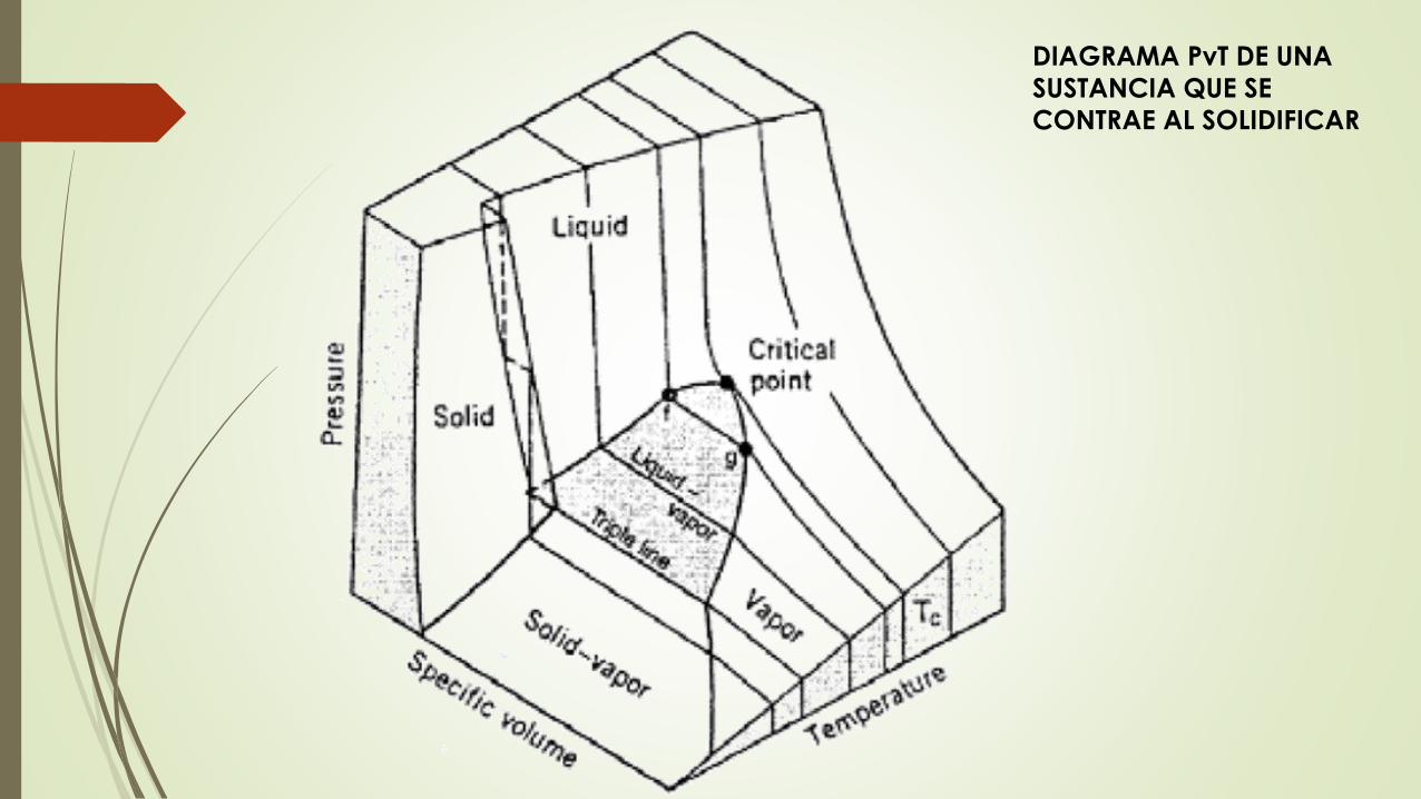
DIAGRAMA PvT DE UNA

SUSTANCIA QUE SE

CONTRAE AL SOLIDIFICAR

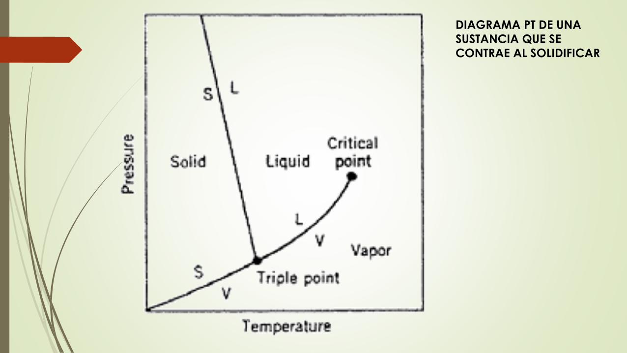
DIAGRAMA PT DE UNA

SUSTANCIA QUE SE

CONTRAE AL SOLIDIFICAR

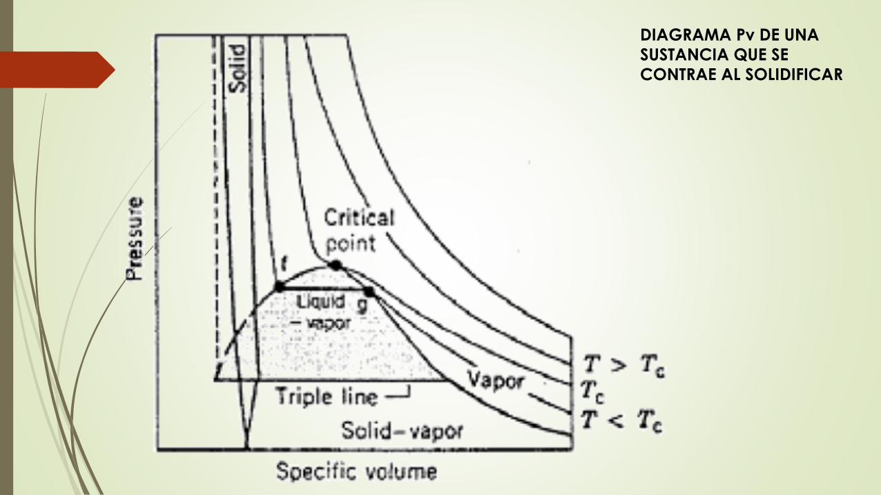
DIAGRAMA Pv DE UNA

SUSTANCIA QUE SE

CONTRAE AL SOLIDIFICAR

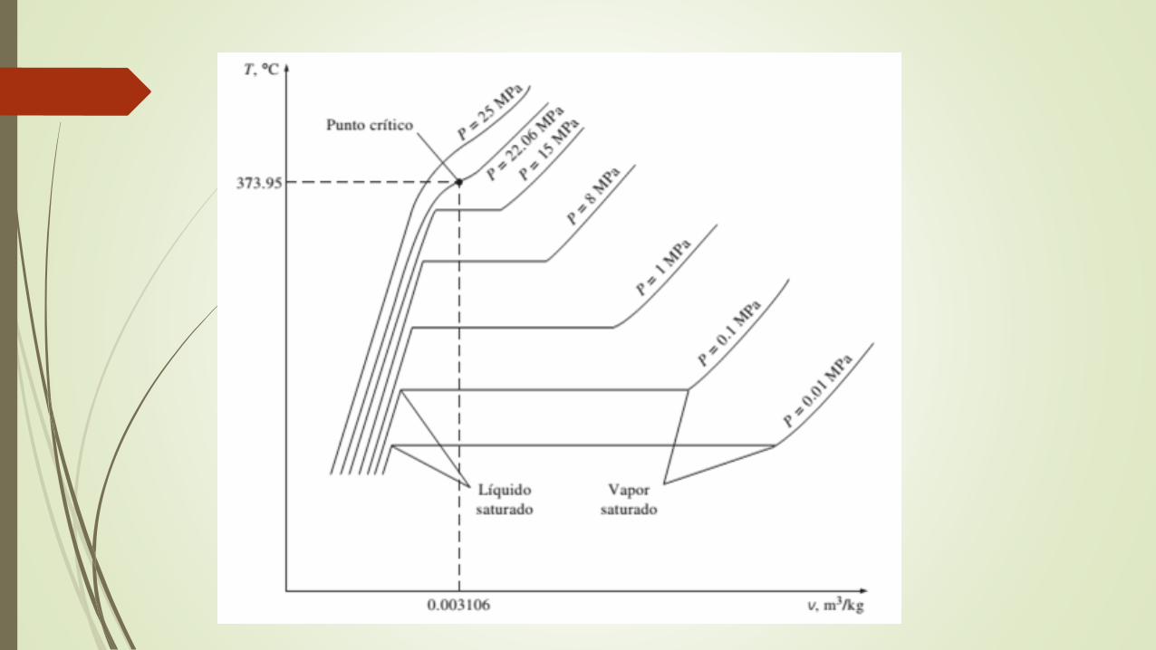
Diagrama de fases de un componente

Se debe especificar el estado termodinámico

de un sistema formado por una sustancia pura,

dado por el número de variables intensivas

independientes (grados de libertad)

Se representa por el diagrama P-T conocido

como diagrama de fases

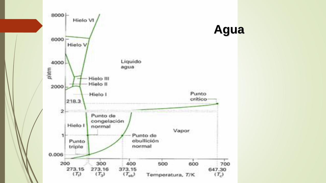
Agua

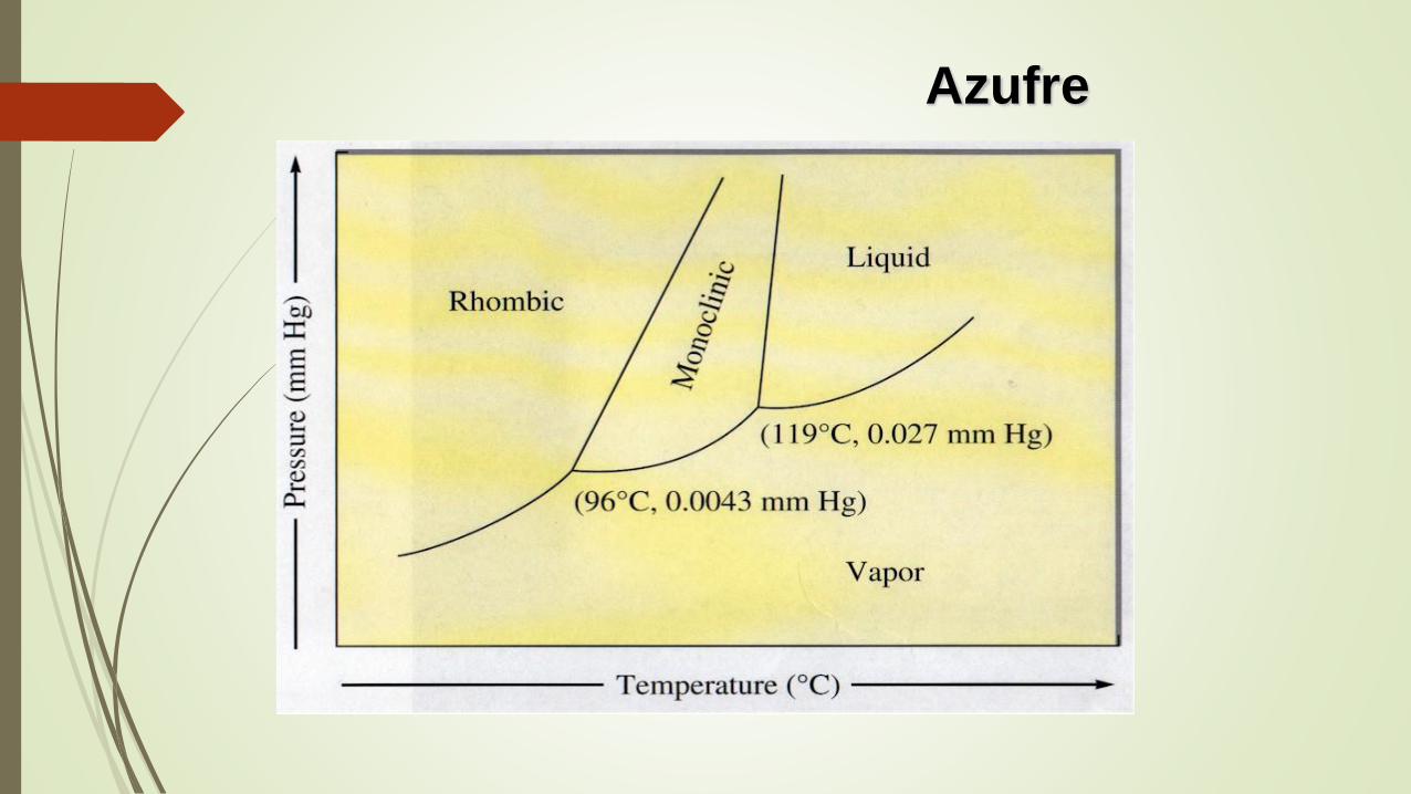
Azufre

600 1000 1400 1800 2200 2600

Temperatura (ºC)

Pre

ssu

re (

GP

a)

Referencias

Tablas y diagramas, Termodinámica técnica I, Termodinámica Técnica II,

Departamento de Ingeniería Energética y Fluidomecánica

Maria Guadalupe Ordorica Morales, Antologia de la asignatura

Termodinámica, UPIBI-IPN, 2006.