INFORME DE LA REUNIÓN INTERSESIONES DE 2018 DEL GRUPO DE ... · de la reunión como inicio para el...

INFORME DE LA REUNIÓN INTERSESIONES DE 2018 DEL GRUPO DE ESPECIES DE ATÚN ROJO SOBRE LA MSE

(Madrid, España, 16-20 de abril de 2018)

"Los resultados, conclusiones y recomendaciones incluidos en este informe reflejan solo el punto de vista del Grupo de especies/Grupo de trabajo /Subcomité. Por tanto, deberían considerarse preliminares hasta que el SCRS los adopte en su reunión plenaria anual y la Comisión los revise en su reunión anual.

Por consiguiente, ICCAT se reserva el derecho a realizar comentarios, presentar objeciones o aprobar este informe hasta que sea finalmente adoptado por la Comisión."

1. Apertura, adopción del orden del día y disposiciones para la reunión La reunión se celebró en la Secretaría de ICCAT, en Madrid, del 16 al 20 de abril de 2018. El Dr. Douglas Butterworth (catedrático emérito de la universidad de Ciudad del Cabo) que ejerció las funciones de presidente para el atún rojo del Atlántico oeste y del Atlántico este y Mediterráneo, inauguró la reunión y deseo la bienvenida a los participantes. El Dr. Miguel Neves dos Santos (Secretario ejecutivo adjunto) se dirigió al Grupo en nombre del Secretario Ejecutivo de ICCAT para dar la bienvenida a los participantes y resaltó la importancia de la reunión como inicio para el proceso de evaluación de estrategias de ordenación (MSE) para el atún rojo. El presidente procedió a examinar el orden del día, que fue adoptado sin cambios (Apéndice 1). La lista de participantes se adjunta como Apéndice 2. La lista de documentos y presentaciones presentados a la reunión se adjunta como Apéndice 3. Los resúmenes de todos los documentos SCRS presentados a la reunión se adjuntan en el Apéndice 4. Los siguientes participantes actuaron como relatores:

Sección Relatores Puntos 1 y 15 M. Neves dos Santos Punto 2 D. Die Punto 3 P. de Bruyn, C. Fernández Punto 4 P. de Bruyn, C. Fernández Punto 5 A. Gordoa, P. de Bruyn Punto 6 C. Fernández, C. Brown Punto 7 N. Duprey, G. Diaz Punto 8 J. Walter, J.J. Maguiere Punto 9 A. Kimoto, S. Miller Punto 10 G. Merino Punto 11 G. Melvin, N. Abid Sección 12 S. Nakatsuka Sección 13 D. Butterworth, D. Die Punto 14 P. de Bruyn

2. Presentación de las cuestiones relacionadas con la evaluación de estrategias de ordenación (MSE)/procedimiento de ordenación

El debate sobre este punto del orden del día tuvo lugar conjuntamente con el grupo de especies de pez espada.

2.1 En qué punto se halla ICCAT en lo que concierne a la MSE

El presidente del SCRS resumió (SCRS/P/2018/019) el contexto en que ICCAT está realizando los trabajos de evaluación de estrategias de ordenación (MSE). Constató que las recomendaciones de ICCAT (Rec. 15-04 y Rec. 15-07) adoptadas en 2015 ponían los cimientos de la decisión de la Comisión con respecto al compromiso con el proceso de MSE para respaldar las normas de control de la captura. La Comisión identificó los stocks prioritarios y en la Rec. 15-04 se encargaba al SCRS el desarrollo de una norma de

REUNION INTERSESIONES MSE - MADRID 2018

1

control de la captura específica para el atún blanco del norte. En la Rec. 15-07 se identificaban los stocks de atún blanco del norte, atún rojo, pez espada del norte y túnidos tropicales como stocks prioritarios y se establecía un plan de trabajo y un calendario que fueron modificados posteriormente cada año por el SCRS y la Comisión. Los cambios al calendario fueron adoptados una vez más en 2017 por el SCRS, que también definió los primeros pasos del trabajo del trabajo técnico que se completará como parte del MSE. Estos pasos fueron detallados en un calendario en el informe de 2017, que reflejaba las fechas más tempranas en las que el SCRS podría proporcionar información suficiente a la Comisión para considerar opciones de normas de control de la captura para cada stock: 2019 para atún rojo; 2020 pez espada del norte y 2021 para túnidos tropicales. El SCRS proporcionó asesoramiento sobre una variedad de las HCR para atún blanco del norte en 2017 y la Comisión adoptó una norma de control de la captura en 2017 (Rec. 2017-04). El presidente del SCRS indicó que en mayo de 2018 el Grupo de trabajo permanente sobre el diálogo entre científicos y gestores (SWGSM) se centrará en la MSE y que se facilitaría una síntesis de los resultados de la reunión actual a dicha reunión para facilitar el debate.

El Grupo agradeció al presidente el resumen expuesto, y acordó tener en cuenta dicha información durante el resto de la reunión.

2.2 Que hace de un MP un MP y de una MSE una MSE

En la presentación SCRS/P/2018/020 se proporciona un resumen de los usos potenciales que podría tener la MSE, de los tipos de estrategias de ordenación están disponibles, así como del asesoramiento sobre las mejores prácticas de MSE.

El Grupo agradeció la presentación realizada en nombre del autor y reconoció su importancia para el proceso MSE de ICCAT. El Grupo resaltó que es importante tener en cuenta las mejores prácticas y reservas con respecto al proceso MSE y a los procedimientos de ordenación (MP) asociados para avanzar en el proceso. Reviste especial importancia la observación clave de que cualquier MP debatido y propuesto debería especificarse clara y totalmente para garantizar que puede reproducirse totalmente y reducir la posible divergencia en su aplicación.

2.3 Mejora de la comunicación: requisito clave para mejorar la eficacia de los procesos MSE

En la presentación SCRS/P/2018/018 se indicaba que el uso de la evaluación de estrategias de ordenación (MSE) para diseñar y probar posibles enfoques de ordenación de pesquerías se está expandiendo a nivel mundial. La participación de gestores, científicos y partes interesadas debería ser un componente integral del proceso MSE. Una comunicación abierta y efectiva entre estos grupos es esencial para el éxito de la MSE y para la adopción de un enfoque de ordenación basado en dicha evaluación. La naturaleza altamente técnica de la MSE y la novedad del enfoque supone para mucha gente un considerable reto de comunicación y, lamentablemente, en algunos casos ha ralentizado los progresos. La presentación se basaba en varias experiencias con la MSE para identificar dos áreas en las que podría mejorarse la implementación de la MSE en un foro multilateral: a) el uso de «grupos de diálogo» formalmente constituidos como foro para el intercambio en la interfaz ordenación-ciencia, y b) el desarrollo de herramientas de comunicación visual atractivas, aunque no complicadas, para transmitir resultados clave a diferentes audiencias en cada fase. Aunque la presentación se centró en los procesos MSE que se están desarrollando en las organizaciones regionales de ordenación de pesquerías para los túnidos y especies afines, el asesoramiento facilitado también era pertinente para otras pesquerías que aplican MSE, tanto a nivel interno como internacional.

También se reconoció que la necesidad de una definición clara de los términos relacionados con la MSE que serán utilizados por el grupo reviste una gran importancia, ya que, de hecho, es necesario estandarizar estos términos entre las diferentes OROP. Existe gran incertidumbre en cuanto al uso de algunos términos, que en muchos casos significan diferentes cosas para diferentes personas. Se observó que esta presentación proporciona un proyecto de glosario de términos dirigido a gestores y partes interesadas. Sin embargo, este glosario no es exhaustivo, y se aconsejó que se prevea la celebración en junio de una reunión del Grupo trabajo conjunto sobre MSE de OROP de túnidos con miras a ampliar este glosario y a añadir definiciones más técnicas.

También es importante la estructura y composición de los diversos grupos que tienen que trabajar para desarrollar una MSE, y se proporcionó asesoramiento en este sentido. Este proceso tiene lugar en cuatro niveles: a) subgrupos que realizan trabajos altamente técnicos proporcionando información científica resumida a b) un cuerpo científico más amplio que encarga de su revisión (como el SCRS) y su discusión en c) grupos intermedios tipo diálogo formales e informales (que incorporan las aportaciones de las partes interesadas) antes de presentar recomendaciones muy resumidas a d) la Comisión. La Secretaría de la


2

Comisión tiene que desempeñar un papel en este proceso y tiene que garantizar una comunicación fluida entre estos grupos, así como la difusión de información vital. Se indicó que las reuniones del SWGSM y de la Subcomisión podrían no ser los grupos intermediarios adecuados para permitir un diálogo real entre científicos, gestores y partes interesadas que potencialmente requieren la formación de grupos adicionales informales, especialmente para los procesos MSE más complejos como, por ejemplo, para el atún rojo del Atlántico.

Para facilitar el proceso MSE en curso, se sugirió encarecidamente que es necesario desarrollar una página web específica de MSE para ICCAT, proporcionando información de contexto sobre los progresos y desarrollos, incluida la información como recomendaciones de ordenación relacionadas con la MSE y plazos, así como información sobre el desarrollo técnico del MSE. El plazo para ello se debatirá más adelante.

También se debatió la necesidad de estandarizar la presentación de los resultados MSE.

El grupo consideró la cuestión de que la definición de objetivos de ordenación (incluido el económico) debería ser un primer paso en el proceso MSE, aunque estos objetivos deben comenzar siendo muy amplios para ir perfilándose después de forma iterativa a medida que los datos y análisis vayan estando disponibles y se van integrando en el proceso. En otras OROP se ha aceptado generalmente que el desempeño de los MP o de las HCR subyacentes es más importante para los gestores que los que los detalles internos de los modelos MP y los modelos operativos de la MSE. Los objetivos y los resultados podrían definirse a nivel de toma de decisiones, pero los aspectos técnicos de la modelación no deberían estar limitados desde el principio.

2.4 Documento de especificación de pruebas de MSE/MP

El contratista externo del grupo de modelación del ICCAT GBYP presentó el documento de especificaciones de pruebas para el atún rojo y expuso información al respecto basándose en los trabajos realizados hasta la fecha por el Grupo de modelación. Se hizo hincapié en que el documento de especificaciones de prueba era un documento vivo que evolucionará con el tiempo y debería actualizarse constantemente. El Grupo acordó que, en este caso, el documento de especificaciones de prueba de atún rojo se actualizará basándose en las recomendaciones de esta reunión. Este documento, tal y como se presentó al Grupo, se incluirá en el Apéndice 7. El Grupo subrayó que deberían desarrollarse documentos de especificaciones de prueba para todas las especies inmersas en un proceso MSE (lo que incluye uno para la MSE de atún blanco del norte, que fue usado para proporcionar asesoramiento a la Comisión en 2017). Para facilitar este ejercicio, se recomendó la creación de un modelo para el documento de especificaciones de prueba, basado en el ejemplo, ya que podría utilizarse para otras especies.

2.5 Ejemplo de los resultados iniciales de MP y su presentación gráfica

En el documento SCRS/2018/047 se proporcionaba información sobre un ejercicio exploratorio inicial en el que se aplicaban normas fijas de proporción simple de control de MP mediante índices de abundancia compuestos para las zonas oriental y occidental, donde estos compuestos consideran promedios ponderados en vez de valores estandarizados de los índices acordados, calculándose a continuación los promedios para los tres últimos años en los que estarían disponibles.

El Grupo indicó que la simplicidad en la presentación de los resultados es clave. Demasiados resultados pueden resultar confusos y complicar las recomendaciones y los resultados. Los gráficos Zeh, los gráficos de gusano y las proyecciones básicas son muy útiles para comunicar información entre los científicos, pero gráficos más simples que muestren las ventajas e inconvenientes de los indicadores clave del desempeño (por ejemplo, captura y estado del stock) aportan probablemente un nivel suficiente de detalle para la Comisión. Se requieren niveles intermedios de detalle para los organismos intermedios previamente identificados

También se debatió la necesidad de reducir el volumen de los resultados del modelo. Deberían retirarse modelos que muestran resultados muy similares ya que la duplicación no es beneficiosa. Además, a menudo podría ser necesario integrar resultados de los diferentes modelos, aunque esto debe hacerse con precaución para no para ocultar o enmascarar cualquier incertidumbre o resultado clave. Además, la ponderación de modelos también es importante, basándose en la verosimilitud relativa. Hay varias maneras de hacer esto con varios ejemplos de otros foros, y estos deberían debatirse y definirse. Se acordó que, al presentar los resultados es mejor no desglosar toda la información, y que sería beneficioso agrupar


3

los resultados en la medida de lo posible (para hacerlos más simples), pero velando porque los detalles importantes no se oculten u omitan.

2.6 LRP en evaluaciones y en MSE/MP (relacionados con el orden del día SWO)

Se informó al Grupo de que el Grupo de especies de pez espada estaba considerando métodos para definir mejor los puntos de referencia límite (LRP) o para verificar que los LRP actualmente adoptados para esta especie son adecuados. El Grupo reconoció que es importante definir exactamente lo que significa un LRP, ya que las diferencias en las definiciones de los diversos foros pueden inducir a confusión. Además, se acordó que un LRP es necesario, pero que tiene que seguir debatiéndose el modo de estimarlo, posiblemente durante las reuniones específicas de especies.

2.7 Respaldo plurianual para la MSE

El Grupo resaltó enérgicamente que es evidente que la MSE es un proceso de varios años (mínimo 2-3 años) que requiere financiación y apoyo técnico a lo largo de su duración. La Comisión tiene que tomar conciencia de este requisito, y los recursos necesarios deben estar disponibles para que el proceso pueda tener éxito.

2.8 Hoja de ruta

El Grupo constató que el calendario MSE del SCRS se había incluido como parte de la propuesta de presupuesto de la MSE (Apéndice 13 del informe del SCRS de 2017). Aunque dicho calendario proporciona información más detallada que la hoja de ruta de MSE de la Comisión (Informe bienal de ICCAT, periodo 2016-2017, Parte I (2016) Vol. 1, Anexo 7.2), el Grupo convino en que se necesitan más detalles para cada proceso MSE y que el calendario tiene que ampliarse a un periodo más largo. La hoja de ruta final debe incluir otros stocks y establecer plazos realistas para cada hito clave con miras a que avancen los procesos MSE (lo que incluye fechas tope: fechas en las que deben tomarse decisiones finales y en las que no se albergará la posibilidad de reconsiderar dichas decisiones). Además, deberían definirse claramente los objetivos/documentos a presentar para los distintos grupos, y deberían planearse las reuniones con bastante antelación para permitir a la CPC prever su participación. Es importante comprender que cada grupo tiene diferentes responsabilidades y proporciona decisiones y recomendaciones con diferentes niveles técnicos y complejidades. El papel de cada grupo de trabajo debe estar claramente definido, y sus responsabilidades de toma de decisiones bien definidas y acordadas. El Grupo subrayó que se requiere más tiempo y reuniones específicas para avanzar en el proceso MSE y que esto no debe realizarse en la periferia de otras reuniones. S e requiere una propuesta para definir el flujo del proceso MSE, que puede basarse en las experiencias de otras OROP/organizaciones en las que la MSE se ha realizado con éxito.

Por último, el Grupo convino en que la hoja de ruta incluye dos tipos de agendas: una a corto plazo para completar la implementación actual de las MSE; otra para la frecuencia de revisiones de los MP (es, decir, revisiones de las MSE). Las fechas para esta agenda de revisión podrían acordarse y finalizarse, pero debería haber un proceso claramente definido para permitir revisiones de las MSE en fechas anteriores (es decir, disposiciones sobre circunstancias excepcionales).

3. Revisión de los documentos disponibles sobre la MSE de atún rojo y actualización del documento de especificaciones de pruebas MSE

Durante la reunión se presentaron varios documentos relacionadas con estas cuestiones. Los resúmenes de estos documentos se incluyen en el Apéndice 4. Las discusiones de estos documentos se incluyen en las secciones pertinentes siguientes. Durante la reunión no se pudo debatir completamente el documento SCRS/2018/041, dado que algunos miembros del grupo de modelación presentaron un documento de respuesta. Los autores del documento SCRS/2018/041, que estuvieron presentes durante la reunión, proporcionaron un documento de trabajo en el que se resumían algunas de sus propuestas para realizar cambios en el documento de especificaciones de pruebas. Las discusiones en la reunión se basaron en este documento de trabajo, dado que no fue posible considerar todas las propuestas realizadas, su consideración ulterior se aplazó a la siguiente reunión. (Véase también la sección 7 de este informe con debates detallados).


4

4. Especificación (priorizada) de los condicionamientos adicionales de OM y presentaciones comparativas de los resultados iniciales de los procedimientos de ordenación candidatos (CMP) que intentarán realizar los expertos en modelación del ICCAT GBYP durante la reunión

El experto en modelación del ICCAT GBYP indicó que se le debería informar lo antes posible de cualquier CMP que deba ejecutarse durante la reunión. Se presentaron cinco CMP durante la reunión. Cada desarrollador de CMP entregó al experto en modelación del ICCAT GBYP su intento de CMP "preferido" hasta la fecha, y se acordó que el experto los ejecutaría durante la reunión y prepararía una representación comparativa de los resultados. A este ejercicio se le asignó la prioridad 1.

Se solicitó al experto en modelación del ICCAT GBYP que preparase un formato común para los gráficos, con el fin de facilitar una comparación de los resultados de los diferentes CMP.

Hubo una solicitud para intentar implementar un “MP de F0,1”, para contar con un escenario que represente la ordenación del statu quo (es decir, la actual). Dicho MP depende del modelo de evaluación de stock utilizado para evaluar el stock. En el marco de la MSE actual no es posible implementar MP basados en una metodología de evaluación de VPA u en otra metodología basada en la edad, dado que la simulación de datos de captura estructurados por talla o estructurados por edad es un tema complejo. Podría considerarse alguna aproximación y se pidió a un subgrupo que propusiese cómo abordar esto en la simulación. El subgrupo sugirió aplicar dos enfoques, basados en interpretaciones de F0,1 independientes de OM y dependientes de OM, respectivamente; los detalles se proporcionan en el Apéndice 5. En discusiones plenarias con todo el grupo, se expresaron diversas opiniones en cuanto a si las sugerencias del subgrupo eran o no apropiadas. El grupo llegó a la conclusión de que intentar un “MP de F0,1”," imitando la estrategia F0,1 de 2017 (basándose en VPA en el este y en VPA/SS en el oeste) no era apropiado en esta fase debido a la falta de datos estructurado por edad generados por el OM y necesarios para construir dichos modelos en el marco del MP. La consideración de la generación de dichos datos no será parte del actual proceso de MSE.

Se planteó una preocupación en cuanto a que, para la zona oeste, los resultados de condicionamiento de algunos OM representados en el documento Carruthers T., and Butterworth 2017 (obtenidos de ajustar el modelo M3, que incluye la mezcla de stocks) parecían muy diferentes de los de la evaluación de stock aceptada para el oeste, con tendencias de la SSB no coincidentes. Por esta razón, se solicitó al experto en modelación del ICCAT GBYP que preparase un OM que fuese más cercano a la evaluación aceptada para el oeste. Antes de hacer este trabajo, con el fin de comprender mejor el rango histórico de variabilidad que abarcan los 12 OM ajustados en Carruthers T., and Butterworth 2017, se preparó un gráfico superponiendo las series temporales de estimaciones de SSB resultantes de este conjunto de OM; se produjeron gráficos separados para las zonas este y oeste, así como para los stocks oriental y occidental. Estos gráficos mostraban que los 12 OM producían diversas tendencias en las series históricas de estimaciones de SSB para el oeste, incluyendo algunas tendencias crecientes recientes, y esto redujo la preocupación planteada inicialmente sobre las tendencias no coincidentes. Se acordó incluir las tendencias de biomasa de la evaluación de stock de 2017 aceptada (VPA para el este y VPA y SS3 para el oeste) en los gráficos y que éstos comenzarán en un año anterior a 1983. La decisión final sobre los resultados coincidentes de la especificación de OM a partir de las evaluaciones de stock acordadas se traspuso al punto 8 del orden del día.

Se observó que los 12 OM de Carruthers T., and Butterworth 2017 estimaban que el estado del stock occidental se ha situado por encima de SSBRMS en todos los años desde 1983 (como se indica en la figura 4 de dicho documento); lo que no coincide con la percepción general que tienen los científicos del historial del stock. Más tarde se informó al Grupo de que los valores SSBRMS calculados hasta ahora por el paquete de software no eran correctos y que los cálculos de SSBRMS de los OM presentados hasta la fecha no deberían tenerse en cuenta. Se corregirá el cálculo de SSBRMS para una versión posterior del paquete. Esto se hará después de esta reunión.

Se observó que los residuos del ajuste a los índices que se muestran en la Figura 3 de Carruthers T., and Butterworth 2017 parecían ser muy similares en los 12 OM ajustados. Aunque el comentario se realizó centrándose en el índice CAN_CMB_RR, esta similitud parecía aplicable a todos los índices y era una característica que ya había sido constatada por el grupo de modelación en su informe de 2017. El experto en modelación del ICCAT GBYP señaló que debe tenerse en cuenta que en los OM cada uno de estos índices se toma para representar la biomasa BFT en un una zona o trimestre específico, en lugar de la biomasa de atún rojo en todas las áreas del este o del oeste; por lo tanto, los residuos de un determinado índice corresponden también a una zona o trimestre específico. Esto, sin embargo, no explica la similitud de los


5

residuos en todos los OM. El experto en modelación del ICCAT GBYP realizó alguna investigación preliminar de esta cuestión durante la reunión, pero indicó que se necesitaba más tiempo para examinar completamente el tema. Proporcionar los diagramas de los ajustes reales a los datos y no sólo los residuos podría aportar información.

Suscitó preocupación que algunos de los resultados inesperados del ajuste de los 12 OM a los datos históricos (es decir, los resultados mostrados en Carruthers T., and Butterworth 2017) podrían deberse a que estas evaluaciones de stock comienzan en 1983, por lo que no se tuvo en cuenta información de años anteriores (por ejemplo, esto podría afectar a las estimaciones de productividad del stock). El experto en modelación del ICCAT GBYP aclaró que para los 12 OM, los cálculos comienzan en el año 1864, estimándose la biomasa y el reclutamiento anterior a 1983 mediante análisis de reducción de stock, debido a la ausencia de datos suficientes de la composición por talla o composición por edad para ajustar los modelos estadísticos de captura por edad y captura por talla. Más tarde, el grupo decidió tratar de remontar la evaluación estructurada por edad hasta 1975 con el fin de utilizar mejor la información disponible. Esto se hará después de esta reunión.

El grupo debatió si es importante que los OM utilizados en las MSE (obtenidos de ajustar el modelo M3, con mezcla de stocks) coincidan con los resultados históricos de las evaluaciones de stock acordadas. Las conclusiones de esta discusión se presentan en el punto 7 del orden del día.

5. Revisión inicial de las experiencias con el paquete de codificación y comentarios Se pidió a los participantes en la reunión que compartiesen sus experiencias con el paquete de software desarrollado por el experto en modelación del ICCAT GBYP. Los participantes que habían probado el paquete antes de la reunión indicaron que en general les parecía muy bueno y fácil de usar. Los comentarios generales fueron los siguientes:

- El paquete genera valores futuros de índices para su uso en los MP. No está claro hasta qué momento

se remontan en el tiempo dichos índices. - Podría ser útil incluir en el manual del software una mejor introducción sobre cómo diseñar un MP,

actualmente está cuestión aparece en cierto modo entreverada en el manual (en la sección 7 del manual). Esto se considera ventajoso, pero de baja prioridad.

- El modelo es extremadamente complejo y, por lo tanto, intensivo computacionalmente. Algunos usuarios tuvieron problemas con los requisitos de memoria computacional. Esto no es sorprendente ya que el modelo M3 contiene 2 stocks, 14 flotas, 3 grupos de edad, fases trimestrales y 10 áreas espaciales. Se están desarrollando rutinas y modificaciones para reducir los requisitos de memoria, pero el tiempo necesario para ejecutar el modelo es inevitable.

- Es importante mostrar el rendimiento de los diferentes OM de manera sencilla y que facilite la comprensión de los resultados y las comparaciones entre los CMP. Se añadirá una aplicación “shiny” al paquete de software. Las formas adecuadas de ponderación para los diferentes OM deben ser consideradas e incluidas en el paquete, además de la aplicación “shiny”, para poder añadir estos resultados a los obtenidos de los OM independientes.

- En relación con el condicionamiento de los OM, más información es necesaria para entender todo el comportamiento y propiedades del modelo M3. El experto en modelación del ICCAT GBYP señaló que un archivo de pdf del informe ya puede ser generado con el software para cada OM ajustado a datos históricos. El archivo muestra la información sobre el ajuste de diagnóstico para los ajustes de los OM a los datos históricos. El experto en modelación del ICCAT GBYP solicitó que el grupo indique si deben mostrarse en el archivo elementos adicionales, por ejemplo, diagnósticos adicionales.

- Se solicitó una aclaración sobre cómo se utilizan los datos (índices) para condicionar los OM, así como sobre cómo los genera el software en la MSE al utilizarlos en los MP. Esto se aborda en la discusión sobre los índices de abundancia descritos a continuación.

- Cuando un TAC se establece para un año y, el último año de datos finalizados en el momento de establecer el TAC es y-2 para las prospecciones e índices de CPUE e y-3 para los datos de captura. Para los años Y-2 e y-1 la captura puede asumirse como igual al TAC. Por lo tanto, el paquete de software no debería permitir el uso de datos para cualquier año posterior a y-2 en los cálculos de los TAC por CMP ya que en realidad estos datos no estarían disponibles en el momento de realizar los cálculos del TAC. Cuando el CMP esté disponible, es importante mostrar los beneficios que conlleva disponer de la información más reciente. Esto puede hacerse mostrando cómo cambia la captura para el mismo nivel de riesgo.


6

- El cálculo de BRMS en la versión de paquete de software disponible para la reunión no era correcto. Una versión corregida se producirá tan pronto como sea posible.

- Es necesario aclarar las opciones para comunicar estadísticas de merma cuando el régimen stock-reclutamiento cambia en el tiempo. La discusión y las conclusiones se resumen a continuación

5.1 Índices de abundancia utilizados para condicionar el OM y especificar el MP

El Grupo solicitó una aclaración sobre los índices de abundancia utilizados para condicionar los OM. Las cuestiones y debates clave fueron los siguientes:

¿Qué índices se utilizan para condicionar (es decir, ajustar a los datos históricos) los OM?

Los índices que se incluyeron fueron los que se muestran en la Tabla 1 (CPUE comercial) y Tabla 2 (índices de prospección) del documento de especificaciones de pruebas (Anexo 1 al Apéndice 7). Se hizo hincapié en que cada índice estaba vinculado a la abundancia de BFT en un trimestre del año y un área espacial específicos. El supuesto "índice principal" en el documento de especificaciones de pruebas puede ser interpretado como una distribución previa de la distribución espacial de atún rojo, pero a continuación los OM se ajustan utilizando los índices de las Tablas 1 y 2 del Anexo 1 al Apéndice 7. Se observó que las CPUE estaban ajustadas solamente desde 1983 en adelante. El Grupo afirmó que podría merecer la pena agregar a la tabla los grupos de edad a los que se aplica cada CPUE para una referencia fácil.

El Grupo señaló que los índices de las Tablas 1 y 2 del Anexo 1 al Apéndice 7 (documento especificaciones de pruebas) no coinciden exactamente con los utilizados en las evaluaciones de stock acordadas, ni se utilizan todos de la misma manera (por ejemplo, algunos índices de series temporales se dividen en la evaluación de 2017 pero no se han dividido en el condicionamiento del OM). Esto se debe en parte a que los índices utilizados para el condicionamiento de los OM se decidieron antes de que se tomaran las decisiones finales en la evaluación de stock en 2017.

Se encargó a un subgrupo revisar los índices utilizados en la evaluación final y proponer cuáles de estos índices (series y periodos) debían ser utilizados en el condicionamiento de los OM. Se observó que el OM es una evaluación espacial, y que los índices utilizados en una evaluación de este tipo no son necesariamente los mismos que pueden ser apropiados en las evaluaciones espacialmente agregadas. También se observó que las evaluaciones de stock acordadas dividen algunas series del índice de abundancia en dos períodos, pero que esa división podría a veces resultar problemática en el contexto MSE porque podría hacer que algunos de los índices de abundancia parecieran mejor de lo que realmente son, lo que tiene implicaciones para el modo en que se generan los índices si se utilizan para proporcionar entradas para los MP). Las conclusiones de todo el grupo tras revisar la propuesta del subgrupo sobre índices se presentan a continuación, y la serie final a utilizar se incluye en el Anexo 1 al Apéndice 7. 1. Si se utilizó el índice en cualesquiera de las evaluaciones de stock acordadas de 2017 (oeste: SS o VPA;

Este: VPA), entonces debe utilizarse en el condicionamiento del OM (excepto cuando se indique expresamente lo contrario), del mismo modo en que se utilizó en SS o VPA. La siguiente sublista resalta los índices específicos que tienen que cambiarse o añadirse al conjunto de índices utilizados en el condicionamiento del OM:

a) Dividir el índice francés de prospecciones aéreas b) Añadir el índice US RR >177 c) Incluir el índice LL GOM 1974-1981 de Japón

2. Cambios con respecto a los índices utilizados en las evaluaciones de stock acordadas:

3. Quitar el índice combinado de Canadá, y sustituirlo por dos índices: SWNS (asignar a WATL) y Golfo

de San Lorenzo (asignar a GSL) ya que estos índices separados incluyen información espacial específica. a) Cambiar la fecha de inicio de todos los índices a 1975. b) En el desarrollo de los CMP, los desarrolladores pueden utilizar los datos para todos los índices

anteriores a 1975 en sus procedimientos de ordenación, manteniendo de este modo la coherencia con los datos facilitados en evaluaciones anteriores.

4. Prueba de sensibilidad/robustez del OM


7

a) Alt. OM: división del índice larvario Med 5. En la reunión de septiembre del grupo de especies de 2018 se considerará recomendar avanzar el año

terminal de lo conjuntos de datos de los índices al 2016 o 2017 para el condicionamiento del OM de la MSE, siempre y cuando estas actualizaciones de datos hayan sido aceptadas antes por la sesión de atún rojo.

Después de la reunión, se volverán a condicionar los OM utilizando los índices acordados durante esta reunión. También se acordó que el "índice principal" debe volver a calcularse basándose en las nuevas opciones de índices. ¿Cómo se proyectan los índices a partir de los OM? Un subconjunto de los índices en las Tablas 1 y 2 del documento especificaciones de prueba (Anexo 1 del Apéndice 7) se proyecta hacia el futuro en cada OM y puede utilizarse para elaborar las CMP. Las propiedades estadísticas (varianza y autocorrelación) de los residuos de los ajustes de OM se utilizan para generar datos de años en el futuro en la MSE asumiendo una distribución lognormal. ¿Cómo se seleccionan los índices que se proyectarán a partir de los OM (y, por lo tanto, estarán disponibles para la construcción de los CMP)? Se aclaró que los principales criterios eran: 1. Probablemente sólo podrán proyectarse 3-4 índices para cada stock, este y oeste, ya que, si se añaden

más, la computación resultaría onerosa. 2. Cada uno debe ser una serie que es muy probable que continúe en el futuro 3. Deben entenderse las propiedades estadísticas de los residuos de los ajustes a los OM, de tal modo que

puedan generarse índices con un comportamiento realista para la MSE. Deberían evitarse los índices que muestren tendencias temporales en los residuos.

4. Son preferibles las series temporales más largas.

Se observó que en el este hay muy pocos índices que cumplan con todos los aspectos de los criterios de selección mencionados para ser incluidos en los índices proyectados por los OM y para estar disponibles para su uso en los CMP. Si se realiza una selección demasiado estricta para los índices del este es probable que no quede ninguno disponible para ser proyectado a partir de los OM y, por lo tanto, se debe dar muestras de cierta flexibilidad en el proceso de selección. El Grupo examinó las implicaciones de la selección de índices de prospecciones para su uso en un CMP si luego estos se interrumpen en el futuro. Si esta situación se produce, el MP podría tener que ser evaluado de nuevo antes de lo inicialmente previsto. Un ejercicio útil, que debe llevarse a cabo en una etapa posterior, es volver a perfilar el CMP asumiendo que ninguna de las tres prospecciones para el oeste esté disponible (de tal modo que solo quede un índice dependiente de la pesquería); se volvería a evaluar entonces el CMP con el fin de mantener el mismo nivel de riesgo y el Grupo podría entonces examinar cuánto tendría que reducirse la captura en ausencia de estas tres prospecciones. Esto justificaría mejor la necesidad de respaldar la continuación de estas prospecciones ante los gestores.

A continuación, se presentan otras conclusiones del Grupo tras revisar la propuesta del subgrupo sobre los índices:

1. Inclusión de índices alternativos proyectados a partir de los OM para las entradas de los CMP (además de los enumerados en el documento de especificación de pruebas) a) Incluir el índice acústico de Canadá como un índice proyectado del oeste a partir de los OM

disponibles para construcción de CMP. b) Una vez que las nuevas diagramas de residuos corregidos estén disponibles para los índices del

este y del oeste, volver a evaluar los índices que se van proyectar en los OM y que estén disponibles para las entradas del CMP.


8

5.2 Comunicación de estadísticas de merma cuando el régimen stock-reclutamiento cambia en el tiempo

El presidente de la reunión sugirió que podría utilizarse un concepto de B0 dinámica1 para comunicar la merma. Esta B0 dinámica se obtendría proyectando la abundancia de atún rojo desde 1864 hacia adelante asumiendo capturas cero en todos los años. Si la relación stock-reclutamiento cambia en un momento determinado, el enfoque de B0 dinámica cambiará los valores de biomasa gradualmente durante un período de varios años, y las estadísticas de merma (B/B0_dinámica) no mostrarán (por ejemplo, la función step) un comportamiento que haga que la interpretación resulte problemática. Se observó que un concepto similar "BRMS dinámica" podría utilizarse, siendo la BRMS dinámica una fracción constante (es decir, invariable en el tiempo) de la B0 dinámica (esto se sostiene para todos los modelos considerados cuando las proyecciones fijan la selectividad por edad en sus valores actuales). Se solicitó al experto en modelado del ICCAT GBYP que preparase un diagrama ilustrativo para la próxima reunión con miras a ayudar a entender la idea.

6. Presentación de los CMP iniciales y resultados asociados por cada persona encargada del desarrollo/conjunto de personas encargadas del desarrollo

NOTA IMPORTANTE: todos los resultados iniciales de los CMP fueron explorados solamente como ejemplos tempranos, es especialmente importante apreciar esto ya que los OM se volverán a condicionar con diferentes índices (ver sección 4) y los índices se ampliarán remontándose hasta 1975 (ya no hasta 1983). Por lo tanto, los resultados se exploraron sólo para fines de discusión y se espera que las tendencias en los resultados podrían cambiar.

Cinco científicos realizaron breves presentaciones que habían preparado CMP antes de esta reunión. La idea era obtener una visión general de los CMP considerados hasta ahora y ver el formato de los diagramas comparativos que se había pedido al experto en modelación del GBYP que preparara. Los resultados de las aplicaciones de los CMP serán diferentes en septiembre, después del recondicionamiento planificado del modelo operativo y otros avances previstos. Por lo tanto, los resultados en este momento se consideraron solo con fines ilustrativos. Todos los CMP presentados se basan directamente en índices de abundancia utilizados en las evaluaciones de stock, es decir, son empíricos más que basados en la estimación/modelo. Se indicó que es posible desarrollar algunos MP basados en el modelo con la estructura existente de los modelos operativos (por ejemplo, MP basados en modelos de producción excedente, como se hizo para el atún blanco del norte). Los detalles técnicos de algunos de los CMP se presentan en el Apéndice 6 de este informe y en los documentos SCRS/2018/P/15; SCRS/2018/P/16; SCRS/2018/P/47; SCRS/2018/55; SCRS/2018/59, pueden encontrarse más detalles. Algunas lecciones aprendidas en este trabajo hasta ahora incluyen lo siguiente: El experto en modelación del GBYP explicó que los modelos del paquete de software hacen referencia a precisión y sesgo en los datos de captura, pero no hacen referencia a cómo se generan los índices de abundancia utilizados en los MP; la generación de índices de abundancia se basa en las propiedades estadísticas de los valores residuales de los ajustes del modelo operativo. El modelo de observación "perfecto" lo utilizan los desarrolladores para hacer pruebas y no está realmente pensado para la presentación final de resultados, si un CMP falla con los datos "perfectos", no debería desarrollarse más. El modelo "bueno" es el que se utiliza por defecto y el modelo "malo" está pensado generalmente como una prueba de robustez. Las discontinuidades en las HCR (como la existencia de umbrales que tienen impactos apreciables en las recomendaciones sobre TAC resultantes dependiendo de en qué lado del umbral caiga una cierta variable) deberían evitarse. Dichas discontinuidades son a menudo problemáticas porque el ruido en los datos o en los resultados puede terminar afectando enormemente a las recomendaciones sobre el TAC. En su lugar,

Algunas CPC utilizaron el término B0 dinámica de un modo diferente al modo en que se define aquí.


9

debería utilizarse una relación lineal desde ligeramente por encima hasta ligeramente por debajo del umbral previsto. Se explicó que ciertos parámetros de las HCR (por ejemplo, un valor del índice objetivo que podría usarse en la norma) a menudo se convierten en parámetros de ajuste en el MP y son elegidos para conseguir un desempeño determinado. El número de años en un periodo de ordenación (el periodo durante el cual se establece un TAC cada vez) podría ser del orden de 2 o 3 años, pero esto debe discutirse con la Comisión. Para este desarrollo inicial de los OM, se impuso un límite de un 20 % a los cambios de TAC interanuales al ejecutar todos los CMP, independientemente de si se especifica en el CMP de manera explícita o no. El Grupo acordó que imponer dicha limitación por defecto en todos los CMP no era adecuado en este momento y que debería eliminarse de los CMP que se están ejecutando. Debería pedirse a los gestores que aporten comentarios sobre el nivel deseado de cambios interanuales en el TAC, aunque estos comentarios es probable que sea mejor pedirlos en una fecha posterior, después de que los resultados iniciales hayan sido presentados a la Comisión. Los comentarios relacionados con los diagramas de comparación presentados por el experto en modelación del GBYP fueron los siguientes. Se consideró que los diagramas presentados por el experto en modelación del GBYP para comparar el desempeño de diferentes CMP con diferentes OM eran muy útiles, aunque se indicó que podría ser difícil interpretar los resultados entre gran número de OM. Debe organizarse un subgrupo (N. Duprey, G. Merino, H. Arrizabalaga, S. Miller, J. Walter, S. Nakatsuka, A. Gordoa, D. Butterworth y A. Kimoto) para trabajar por correspondencia sobre la mejor forma de presentar los resultados en las próximas reuniones científicas. El subgrupo presentará un informe a la próxima reunión de este grupo de trabajo sobre MSE para el atún rojo. Algunos pensamientos iniciales fueron: - Para los CMP considerados, las diferencias en el desempeño entre los OM eran generalmente mayores

que las diferencias entre los CMP. El Grupo examinó los diagramas sobre el nivel de captura global, la variabilidad interanual de la captura y la resultante merma del stock. La captura y la variabilidad de la captura deberían comunicarse por área, mientras que las estadísticas de merma deberían comunicarse por stock. También podría ser interesante comunicar la abundancia de atún rojo por área.

- La variabilidad interanual de la captura debería tenerse en cuenta al examinar los resultados, ya que

podría tener impactos importantes operativos y de ordenación, a menudo la industria pesquera está a favor de bajos cambios interanuales en el TAC, aunque no es siempre así. La información mostrada en los diagramas se basaba en medias del periodo de proyección de 30 años modelado. El Grupo consideró que sería útil incluir diagramas adicionales mostrando la información sobre la Variación media anual por separado para los aumentos y descensos interanuales en la captura, es decir, teniendo en cuenta el signo, así como la magnitud de los cambios.

- Entre los OM para los que se presentaron resultados, el OM que incorporaba un cambio de régimen

implicaba el mayor riesgo para el stock del este, y por esta razón es crucial considerar el escenario de un cambio de régimen para identificar CMP adecuados para el atún rojo.

- Los diagramas deberían examinarse para buscar resultados que puedan parecer sospechosos

teniendo en cuenta los conocimientos de los expertos acerca de la dinámica y la productividad del atún rojo, por ejemplo, lo MP que conducen a capturas elevadas hasta un nivel que se ha visto que era insostenible en el pasado deberían dar lugar a una investigación cuidadosa de los OM asociados.

- Se produjeron algunos casos en los que los intervalos de probabilidad en la captura media proyectada

eran muy pequeños y los responsables del desarrollo deberían examinar con cuidado los MP afectados para intentar comprender qué causa esto. Por el contrario, los CMP con grandes intervalos de probabilidad en la captura media proyectada o que cubren una amplia gama de niveles posibles de


10

capturas/merma podrían ser problemáticos y el responsable de desarrollar el CMP debería explorar más en profundidad qué características de sus CMP podrían estar causando esto.

- Criterios de evaluación para los CMP: Un CMP que dé lugar a una merma del stock hasta niveles muy

bajos es obviamente un fracaso. Sin embargo, aún no se han desarrollado orientaciones sobre niveles de merma que generen inquietud (por ejemplo, puntos de referencia límite, umbral) ni se cuenta con otros criterios objetivos para determinar lo que constituye un fracaso (o un éxito). Se consideró que sería mejor esperar hasta que se implementen los cambios planificados a los OM y los CMP (es decir, como mínimo hasta septiembre de 2018) para que se entienda mejor el margen de lo que es viable antes de establecer unas directrices más específicas.

7. Desarrollo de un formato estándar para una comparación fácil de los resultados clave entre los

diferentes CMP y sus pruebas Debido a limitaciones de tiempo, el Grupo acordó posponer la discusión de este tema. Para facilitar las discusiones futuras, el Grupo solicitó que el Dr. Carruthers y los siguientes miembros del Grupo: N. Duprey, G. Merino, H. Arrizabalaga, S. Miller, J. Walter, S. Nakatsuka, A. Gordoa, D. Butterworth y A. Kimoto trabajen en el periodo intersesiones para desarrollar una propuesta que se presentará en la próxima reunión del Grupo. 8. Posibles modificaciones del paquete de codificación y de sus pruebas asociadas

(SCRS/2018/041) y respuesta, y plan de trabajo en preparación Como se ha indicado en la sección 4, el conjunto de OM presentado a la reunión en el documento sobre Especificaciones de los ensayos y en Carruthers T. y Butterworth, D., 2017 serán recondicionados después de esta reunión utilizando los índices acordados durante la reunión. Se expresó la inquietud en el Grupo de que no se entendía lo suficiente el comportamiento de los OM y de que los OM podrían mejorar con algunos cambios en las especificaciones de los datos de entrada (SCRS/2018/041). Tras revisar los OM existentes, el Grupo realizó varias modificaciones recomendadas para reflejar mejor la naturaleza de las incertidumbres (Tabla 7.1). El Grupo discutió y acordó también cambios que se implementarían en el conjunto de OM de referencia y en los ensayos de robustez (utilizando la terminología de la sección 9 del documento sobre especificación de los ensayos). Estos cambios se presentan en las siguientes secciones: 8.1 Condicionamiento general de OM Para poder usar la serie completa del índice larvario del GOM (1977-presente) y para reflejar mejor un periodo más largo de la dinámica del stock, el Grupo acordó que el condicionamiento del OM debería empezar en 1975. 8.2 Escenarios de reclutamiento utilizados en los OM

- Para el oeste, el escenario de "alto reclutamiento" (nivel 2 del eje 1 de incertidumbre "reclutamiento

futuro" en el conjunto de OM de referencia en el documento de especificación de ensayos) no fue capturado correctamente en el OM y debe ser especificado de nuevo. Cualquier resultado observado para este escenario debería ser, por tanto, descartado. El problema era que se estaba estimando un nivel muy elevado de inclinación (h), lo que originaba una diferencia muy pequeña entre la dinámica del bastón de hockey y la dinámica del stock-reclutamiento (SR) alto. En la reunión se acordó utilizar h = 0,6, que generalmente se encuentra dentro del rango de la inclinación estimada en evaluaciones de stock anteriores de atún rojo del oeste. Se resaltó que los escenarios de reclutamiento considerados en el conjunto de OM de referencia debían capturar un rango representativo de incertidumbres, pero no implican ninguna ponderación relativa en particular entre los diferentes escenarios (este tema que se discutirá en una reunión posterior). Es también esencial garantizar que la relación stock-reclutamiento para el escenario de alto reclutamiento tiene un reclutamiento virgen (R0) que es sustancialmente más alto que la del palo de hockey.


11

- Se acordó también fijar el punto de bisagra de la relación stock reclutamiento en forma de bastón de hockey utilizada para el stock del oeste de acuerdo con especificaciones similares a las utilizadas en evaluaciones anteriores, por ejemplo, el umbral de la SSB (bisagra) se estableció en la SSB media durante un periodo (generalmente 1990-1995) con la SSB estimada más baja y R0 se calculó como la media geométrica del reclutamiento durante el periodo después de 1976 (Anón. 2014).

- Se indicó también que el nivel 3 del eje de incertidumbre 1 "reclutamiento futuro" en el conjunto de

OM de referencia está pensado para reflejar un posible cambio de régimen en el reclutamiento. En el oeste, podría haber ocurrido un cambio de régimen en 1975 y en el este entre 1987 y 1988. En el oeste, el palo de hockey (nivel 1) es un escenario pensado para reflejar que se ha producido un cambio de régimen a un régimen de bajo reclutamiento, mientras que el Beverton-Holt (nivel 2) asume que el reclutamiento puede aun ser potencialmente muy alto. Se explicó que las experiencias pasadas indicaban que el escenario del cambio de régimen (nivel 3) es crucial para garantizar que se identifican los MP con un buen desempeño. Las implicaciones metodológicas de los cambios de régimen para las evaluaciones del desempeño de los MP ya se discutieron en el párrafo "dinámica B0" anterior de este informe.

- El Grupo se mostró de acuerdo en que era necesario un texto adecuado en el documento sobre

especificación de ensayos y en los diagramas de los ajustes stock-reclutamiento, así como de las tendencias en el reclutamiento consideradas para cada OM con el fin de explicar la base de los escenarios de reclutamiento elegidos para el conjunto de OM de referencia.

- Se indicó también que los cálculos de SSBRMS debían rehacerse como parte del recondicionamiento del

OM.

Escenarios de abundancia y medida en la que los resultados de condicionar los OM debería corresponderse con los de las evaluaciones de stock acordadas: El eje de incertidumbre 2 ("abundancia") en el conjunto de OM de referencia presentado por el experto en modelación del GBYP contiene escenarios (niveles B y C) en los que los resultados de condicionar los OM fueron "obligados" a igualar ciertas características de las evaluaciones de stock de 2017. El Grupo discutió si dicha equiparación es adecuada y consideró adicionalmente posibles modificaciones a los escenarios examinados bajo este factor. Se produjo un acuerdo general respecto a que deberían preverse las diferencias entre los OM y las evaluaciones de stock acordadas porque los OM contenían muchas más características, como la disgregación espacial y la mezcla de lo stocks, que no estaban incluidas en las evaluaciones de stock de 2017. Sin embargo, los resultados de condicionar los OM deberían ser cuidadosamente revisados para comprobar si existen discrepancias importantes con los amplios conocimientos de los científicos sobre la dinámica global del stock de atún rojo. En particular, es más fácil que los resultados sean aceptados si al menos algunos de los OM reflejan en cierta medida la percepción pública de las tendencias del stock. Por ejemplo, algunos OM para ambas zonas del stock deberían mostrar que se ha producido sobrepesca y que los stocks han estado sobrepescados durante algunos periodos. Otro ejemplo sería el Atlántico oriental, donde los OM no deberían mostrar incrementos en la biomasa en los momentos en los que las capturas eran del orden de 50.000 t por año. Por ello, el Grupo recomienda tres propuestas para abundancia. PROPUESTAS: Se acordó que el conjunto de OM de referencia debería contener al menos 3 escenarios para el eje 2 de incertidumbre "abundancia".

A. Mejor estimación del ajuste del OM. Si esto implica grandes diferencias con las evaluaciones aceptadas, debería identificarse la razón para las diferencias.

B. Las tendencias y escalas en SSB que resultan de condicionar el OM para el este y el oeste son obligadas simultáneamente a seguir estrechamente los resultados de las evaluaciones del stock de 2017 en términos tanto de magnitud absoluta como de tendencia (deberían utilizarse para esto las evaluaciones de stock acordadas por el SCRS en 2017). Esto debería ayudar a identificar la razón de cualquier posible diferencia identificada en A.

C. Esto es similar al escenario A, pero incluyendo algunas limitaciones amplias para impedir que los resultados de condicionar el OM diverjan del actual conocimiento general de la pasada dinámica del stock. El Grupo consideró que sería adecuado requerir que los resultados del OM para el atún


12

rojo tanto del este como del oeste muestren que han estado sobrepescados en algún momento del pasado. Esto significa no sólo que la biomasa del stock reproductor es inferior a SSBrms, sino también un nivel de SSB relativamente bajo en ciertos periodos. Podría considerarse también evitar aumentos en la SSB durante pasados periodos de capturas elevadas, lo que debería ser claramente explicado si se incluye en el escenario. Estas ideas quieren reflejar la percepción pública de que el atún rojo se encontraba en un nivel bajo (especialmente en el este) hacia el cambio de siglo. Se dio cierta flexibilidad aquí al experto en modelación del GBYP, dependiendo de los resultados de varias exploraciones.

El experto en modelación del GBYP solicitó que el Grupo indicara los tipos de diagnóstico que desearía ver y debatir para sentirse cómodo con un OM. Muchos diagnósticos actuales están disponibles en los informes específicos del modelo operativo que proporcionará el experto en modelación del GBYP. 8.3 Movimiento y mezcla de los stocks Se mantuvieron importantes discusiones para aclarar cómo se modela el movimiento en los OM (los OM tienen una probabilidad de movimiento entre zonas espaciales dependiente del stock de origen y la edad que cambia de trimestre a trimestre, pero es la misma para todos los años). Se produjeron sustanciales discusiones sobre la medida en la que este supuesto puede considerarse realista, aunque comprendiendo que los datos disponibles para estimar el movimiento variable en el tiempo son limitados. Aunque en los OM se asume que las tasas de movimiento para una edad, stock y trimestre determinados son constantes de año en año, la composición del stock en cualquier región, trimestre y año es variable. El OM utiliza los ajustes a los datos disponibles de marcado electrónico, así como información genética y sobre microquímica de otolitos para estimar las tasas de movimiento, y cabe señalar que todos los datos utilizados para ajustar el OM contribuyen en alguna medida a la estimación de las tasas de movimiento. Cabe destacar que los datos de la composición del stock obtenidos para la región GSL canadiense sobre genética muestran una mayor representación de atún rojo del stock oriental en años recientes. Podrían considerarse otros escenarios de movimientos en el OM como aumentar el peso del GSL en el modelo de gravedad, o permitir tasas de movimiento que varíen en el tiempo, pero dadas las limitaciones temporales y el contenido informativo de los datos, se acordó mantener el escenario de movimiento de referencia utilizado hasta ahora (por ejemplo, mismas probabilidades de movimiento en todos los años). Se señaló el creciente porcentaje de peces originarios del este en el GSL, por lo que separar los índices GSL y SWNS en los OM (véase sección 4) podría solucionarlo. Existe la inquietud de que las tasas de movimiento puedan estar sobrestimadas por el ajuste a los datos observados de composición del stock, ya que los datos de composición siempre tienen algún elemento de incertidumbre y a menudo tienen una fracción no despreciable de un stock mucho menor, incluso en zonas donde se ha asumido anteriormente que no se produce mezcla. Por ello, las tasas de movimiento podrían estar sobrestimadas y los modelos espaciales, con el fin de mejorar los ajustes, podrían situar biomasa en zonas donde no se pesca actualmente basándose en información de marcado electrónico. El Grupo prefería que el conjunto de OM de referencia abarque escenarios alternativos de mezcla. Dada la complejidad de desarrollar escenarios alternativos, el Grupo resaltó varias propuestas. Inicialmente, algunos se propusieron para incluirlas en el eje de incertidumbre al desarrollar el conjunto de OM de referencia, sin embargo, debido a inquietudes respecto al aumento del número de OM (lo que dificultaría la presentación de los resultados y el funcionamiento de la MSE), la propuesta se modificó para incluirlos como parte de las pruebas de robustez. Existe, sin embargo, la expectativa de que, si los OM alternativos de la mezcla cumplen los criterios de desempeño, podrían ser reclasificados en el conjunto de referencia en una reunión posterior. PROPUESTAS: El Grupo acordó dos escenarios de mezcla (i y ii a continuación) y un cambio al tratamiento de los datos de marcado (iii a continuación): i) Reducir a la mitad la mitad de las tasas de mezcla, por ejemplo, si la fracción observada de peces

originarios del oeste en un trimestre/área/año asumido como oriental es del 40 %, este escenario asumirá que es solo del 20 %. Dichos cambios reducirán las tasas estimadas de movimiento entre el este y el oeste y podrían representar un escenario plausible. Este conjunto de OM se utilizará para el conjunto de robustez, con gran prioridad.


13

ii) Condensar el modelo de 10 áreas en un modelo de 7 áreas juntando las 6+7, 5+9 y 1+2. Se recomienda también añadir esto como prueba de robustez, indicando sin embargo que esto también corresponde a un cambio estructural en el modelo que tiene importantes implicaciones de código y por tanto se le concede una prioridad relativamente baja.

iii) El Grupo acordó también que el marcado de juveniles por parte de AZTI en el golfo de Vizcaya se utilizará para estimar las tasas de movimiento, asumiendo que dichos peces son originarios del este, basándose en previos estudios de química de otolitos que así lo sugieren (Fraile et al., 2014). Este cambio se hará en todos los OM.

El Grupo consideró varias opciones para diferentes escenarios de mezcla, como el uso de solo una fuente de información sobre la mezcla cada vez (por ejemplo, microquímica o solo ADN) o permitir tasas de movimiento que varíen con el tiempo o tasas de mezcla media (Hazin et al., 2018), pero en este punto estas opciones no se consideraron para los OM alternativos. El Grupo discutió también sobre el hecho de que se sabe las evaluaciones de stock de VPA acordadas son sensibles a la ratio de F asumida, lo que apunta a un nivel desconocido de biomasa críptica. Se expresó la inquietud respecto a que grandes cantidades de biomasa críptica podrían afectar a los OM, moviendo grandes cantidades de peces fuera del rango de la pesquería. Para solucionar esto, el Grupo acordó que la distribución espacial de la biomasa vulnerable y no vulnerable (críptica) por stock en cada zona debería ser representada gráficamente a lo largo del tiempo. 8.4 Capturabilidad e índices Observando que las recomendaciones para los índices utilizados en el condicionamiento del OM histórico se han reflejado en la sección 4, en esta sección del informe solo se discuten aspectos de las especificaciones de índices futuros. PROPUESTA:

A. Aplicar un aumento del 2 % en la capturabilidad para los índices proyectados de CPUE dependientes de la pesquería en una prueba de robustez.

Esta propuesta es aplicar un aumento del 2 % en la capturabilidad para los componentes previstos de los OM para proteger frente a la merma no detectada. Esto se aplicará como una prueba de robustez. Esto se aplicaría solo a los índices del tamaño del stock dependientes de la pesquería. Se asume que los índices del tamaño del stock independientes de la pesquería tendrán capturabilidad constante. Si los métodos para recopilar los índices del tamaño del stock independientes de la pesquería se cambian en el futuro, se asume que se derivará un coeficiente de calibración en el momento en que ocurra. El valor del dos por ciento se basa en el cambio estimado en la capturabilidad para uno de los índices del tamaño del stock durante un periodo de 45 años. El Grupo observó que la capturabilidad no aumenta necesariamente siempre. Para algunos índices, los factores medioambientales podrían rebajar la capturabilidad y los cambios en la capturabilidad no se prevé necesariamente que sean monótonos. El Grupo sugirió que estos cambios, incluidos los cambios más drásticos en la capturabilidad, se incluyeran en una prueba de robustez como segunda prioridad. Se consideró una propuesta para incluir la varianza específica de los índices, la autocorrelación y la no linealidad de los índices proyectados. Se expresó la inquietud respecto a que el método de estimación de la autocorrelación y la no linealidad podría haber sido inadecuado y que estas estimaciones deberían ser examinadas de nuevo para un Documento de especificación de ensayos revisado. Una vez que el procedimiento de estimación haya sido finalizado y el recondicionamiento completado conforme a las decisiones tomadas en esta reunión, el Grupo acordó volver a ejecutar la estimación de la autocorrelación y la no linealidad y, si se justifican estadísticamente, utilizarlas en una prueba de robustez. 8.5 Resumen de los cambios propuestos al OM En general, el Grupo recomienda los siguientes cambios a los OM (Tabla 1 a continuación) y se indican de acuerdo a si aplican a todos los OM, solo al conjunto de OM de referencia o solo al conjunto de OM de robustez.


14

Conjunto de referencia Tres ejes principales de incertidumbre: reclutamiento futuro, abundancia y mortalidad natural/madurez (en combinación) para el condicionamiento y las proyecciones. Estos ejes asumen que las opciones del este y el oeste están vinculadas en las filas de la tabla a continuación. Esto se hace con la intención de capturar los extremos. Tabla 1. Cambios recomendados al conjunto de OM de referencia

Oeste: Este:

Reclutamiento futuro

1 Palo de hockey con un punto de bisagra fijado a partir de 1975. 88+ B-H con h=0,98

2 B-H con h=0,6 fijado, elevado R0* 88+ B-H con h=0,70

3 Palo de hockey cambia a B-H después de 10 años

88+ B-H con h=0,98 cambios a 50-87 B-H con h=0,98 después de 10 años

Abundancia A Mejor estimación

B Las biomasas reproductoras de la zona este-oeste coinciden con la evaluación del VPA de 2017.

C Distribución a priori en la tendencia y/o en la merma para que se corresponda con la percepción de explotación muy elevada.

Fracción reproductora ambos stocks Tasa de mortalidad natural ambos stocks I Más jóvenes Alto II. Más jóvenes Bajo III. Mayores Alto IV. Mayores Bajo

* El reclutamiento alto debería reflejar un R0 mayor que el palo de hockey.

Combinación del conjunto de referencia Un cruce completo de (1, 2, 3) x (A, B, C) x (I, II, III, IV), es decir, 36 escenarios en total. Cambios recomendados al conjunto de OM de robustez (Apéndice 7, sección 9b) Prioridad alta

1. Robustez ante menos mezcla (50 %): diseño cruzado con 4 pruebas correspondientes a 1A, 2A, 1B, 2B en la Tabla 1 anterior.

2. Las capturas futuras en el oeste y en el este+Med son cada año 20 % mayores que el TAC como resultado de la pesca IUU (de lo cual el MP no es consciente).

3. Un aumento no detectado en la capturabilidad futura para los índices de abundancia basados en la CPUE del 2 % por año.

4. Relaciones índices-abundancia no lineales: revisar las estimaciones basándose en una estimación estadística más adecuada y revisar los componentes de la proyección de los OM.

5. Robustez ante más mezcla: diseño cruzado con 4 pruebas correspondientes a 1A, 2A, 1B, 2B en la Tabla 1 anterior.


15

Prioridad baja

1. Modificación del reclutamiento futuro como en 3), pero con una probabilidad del 0,05 para cada uno de los 20 primeros años de la proyección.

2. Asignaciones alternativas del stock de origen de las capturas históricas del Atlántico sur (aguas de Brasil).

3. Modelo de siete áreas. Condensar el modelo de 10 áreas en un modelo de 7 áreas juntando las 6+7, 5+9 y 1+2.

Temas de "segunda ronda" (no en este actual proceso de MSE) Se recomienda aplazar en este momento para su consideración en una "segunda ronda" los siguientes aspectos de incertidumbre:

1. Más de dos stocks 2. Uso de datos CAL (CAS en ICCAT) en un MP. 3. TAC asignados de forma espacialmente más compleja que el tradicional oeste y este+Med. 4. Cambios en las medidas técnicas que afectan a la selectividad 5. Cambios en las distribuciones del stock en el futuro 6. Cambios futuros en la asignación proporcional de los TAC entre las flotas.

9. Presentación de los resultados de posibles mejoras de los CMP desarrollados durante la reunión

Debido a limitaciones de tiempo y a la necesidad de hacer en primer lugar correcciones a los OM del paquete de codificación, no se realizaron más mejoras a los CMP presentados durante la reunión. 10. Acuerdo para una especificación de calibración (posiblemente más de una) para facilitar la

comparación de los resultados futuros que se presenten (por ejemplo, mediana del nivel objetivo de la biomasa al final del periodo de proyección para cada una de las poblaciones del este y del oeste para una prueba específica única)

En el Apéndice 8 se presenta una explicación completa de la calibración. El Grupo indicó que el desarrollo de un valor del parámetro de control de la calibración será específico para cada uno de los dos stocks. Cada desarrollador podrá decidir su propia calibración preferida. El ajuste del desarrollo por separado es para ayudar a diferenciar el desempeño de dos CMP en condiciones en las que su mediana de la merma después de 30 años es la misma. Para la calibración del desarrollo, en un ensayo particular cada desarrollador lo calibrará para obtener la mediana de SSB/SSBRMS=1 en el año 30 de la proyección para un OM central además de su propia calibración preferida. Este ejercicio será de uso interno entre los desarrolladores y el grupo de MSE. Al presentar los resultados a los responsables de la toma de decisiones, se hará una media de las mediciones del desempeño entre los OM. 11. Discusiones iniciales y especificaciones de los aspectos en los que las aportaciones de la

Comisión/las partes interesadas sean susceptibles de contribuir a la mejora de los CMP (esto está relacionado, en parte, con un mayor detalle en lo que concierne a los objetivos y ventajas e inconvenientes)

La reunión de SWGSM (21-23 de mayo de 2018) contará con un punto del orden del día específico para la MSE del atún rojo (punto 6.2). El objetivo es que las partes interesadas comiencen a realizar aportaciones


16

para ayudar en la futura mejora de los CMP. Además, es necesario proporcionar alguna orientación a la Comisión sobre la hoja de ruta general de ICCAT para la MSE y recomendaciones sobre MSE. Las aportaciones al SWGSM serán en forma de una síntesis del informe de esta reunión. El presidente del SCRS preparará dicha síntesis y la circulará a todos los participantes en esta reunión antes del 28 de abril. Los comentarios sobre dicha síntesis deberán recibirse antes del 5 de mayo. Después, el presidente del SCRS modificará el informe y lo pondrá a disposición de todos los participantes (incluidos los participantes en el SWGSM) antes del 9 de mayo2. La síntesis tendrá los siguientes objetivos: Actualización del estado del trabajo relacionado con la MSE realizado por el SCRS - Resumir el progreso del trabajo realizado hasta la fecha y demostrar la importancia de continuar

dotando de recursos al trabajo sobre MSE del GBYP. - Proporcionar información suficiente y comprensible para garantizar que las aportaciones de los

participantes en el SWGSM son útiles y aumentar el compromiso de los participantes en el SWGSM en el trabajo sobre MSE que lleva a cabo el SCRS.

- Remitir a la Comisión un calendario realista para finalizar la MSE. Basándose en otras experiencias, incluso en una situación muy optimista, el Grupo de especies de atún rojo probablemente necesitará al menos cuatro reuniones más de una semana dedicada a esta MSE. El calendario actual, que sugiere completar la MSE antes de 2019, debe ser revisado en consecuencia.

Consideración de posibles procedimientos de ordenación (CMP) - Describir los tipos generales de características de los MP que se están proponiendo para que los

participantes en el SWGSM puedan aportar comentarios: • Si dichos tipos de MP son aceptables • Posibles limitaciones en el TAC • Los objetivos globales para los MP en términos generales (por ejemplo, prioridades entre

la conservación de los recursos, maximizar las capturas y minimizar el alcance de los cambios al TAC, con asesoramiento sobre los intervalos preferidos entre los cambios al TAC).

- Entender cuándo será útil y necesario contar con más aportaciones sobre objetivos de MP más detallados. Transparencia y comunicación de los resultados de MSE - Obtener orientaciones sobre posibles modificaciones al actual proceso de MSE para mejorar la

comunicación de los resultados de MSE y la implicación de los participantes en el SWGSM en el desarrollo de la MSE.

12. Programa de trabajo para una ulterior mejora del CMP, con plazos, que genere los resultados

buscados para su presentación al grupo de especies de atún rojo de septiembre de 2018 El Grupo sugirió provisionalmente el siguiente calendario de trabajo a corto plazo. El Grupo discutió intensamente la viabilidad de la reunión del Grupo de septiembre (punto 5) y se plantearon muchas inquietudes respecto al ocupado calendario de reuniones. La Secretaría explicó que mover la fecha de la reunión significaría modificar el contrato de modelación del GBYP. El propósito general de dicha reunión se entendía como foro para más discusiones sobre el recondicionamiento de los OM y para examinar los resultados de los CMP revisados, continuando las discusiones de esta reunión.

1. Finales de mayo - Finalización de las actualizaciones del OM en base a esta reunión (experto en modelación del GBYP)

2. Mediados de junio - Comentarios sobre los OM actualizados

2 Este informe fue finalizado el 9/5/2018 y en ese momento no se habían cumplido los plazos y el presidente del SCRS debía preparar el documento de síntesis.


17

3. Principios de julio - el experto en modelación del GBYP circula el paquete actualizado en base a las revisiones finalizadas

4. Mediados de julio a principios de septiembre: a) Los desarrolladores vuelven a ejecutar los CMP ajustados en el paquete actualizado; b) Documentos preparados sobre temas del condicionamiento que requieran atención.

5. Las actividades que se producirán después de principios de septiembre se regirán por las recomendaciones de la sección 13. Las decisiones a este respecto las tomarán el presidente del SCRS, los relatores de atún rojo y la Secretaría.

13. Recomendaciones El Grupo identificó varios desafíos a los que se enfrenta el Grupo de especies de atún rojo a la hora de participar e implicarse de manera eficaz en el proceso de MSE para el atún rojo: - La necesidad de mecanismos, lo que incluye reuniones bien planificadas, que faciliten la participación

del Grupo de especies de atún rojo a diferentes niveles y que garanticen que se mantiene el impulso del proceso de MSE.

- Las dificultades encontradas por los miembros del Grupo de especies de atún rojo para involucrarse de manera efectiva en el proceso anteriormente a causa de las demandas impuestas por la evaluación del stock de atún rojo de 2017.

- La mejor forma de lograr una mayor participación del Grupo de especies de atún rojo en el proceso de MSE sería mediante reuniones del grupo que sean largas (de más de 3 días) centradas únicamente en la MSE.

- Las dificultades a las que se enfrentan muchas CPC para involucrarse de manera efectiva en las múltiples sesiones simultáneas durante la semana de los grupos de especies en septiembre a causa del limitado número de científicos en las respectivas delegaciones de las CPC.

- La duración adicional del tiempo fuera de casa generada al añadir días de reunión antes de la semana de los Grupos de especies.

Teniendo en cuenta estos problemas, el Grupo recomienda lo siguiente: - La decisión sobre el número de días de reunión asignado a la reunión de septiembre del Grupo de

especies de atún rojo, el orden del día de dicha reunión y el calendario para la próxima reunión del Grupo de modelación deberían considerar los problemas mencionados.

- En las reuniones futuras del Grupo de modelación debería fomentarse la participación de cualquiera interesado en realizar aportaciones al proceso de MSE.

- Los objetivos y el orden del día de cualquier reunión del Grupo de modelación deberían ser ampliamente circulados entre todo el SCRS con bastante antelación para ayudar a la participación de todos los científicos interesados en dicha reunión.

- A principios de 2019 el SCRS celebrará una reunión intersesiones de una semana del Grupo de especies de atún rojo centrándose en la MSE.

En otro punto de este informe se incluyen recomendaciones específicas para el desarrollador de la MSE de atún rojo y el Grupo de modelación. Hay unas pocas recomendaciones generales al SCRS relacionadas con la experiencia adquirida con la MSE del atún rojo: - Otros procesos de MSE en el SCRS deberían considerar las ventajas que el marco de MSE desarrollado

por el GBYP podría tener en sus propios procesos de MSE. Dichas ventajas incluyen la aplicación actual de este marco a un stock de ICCAT, el poder y la flexibilidad de los diferentes módulos del marco y la experiencia adquirida por varios científicos del SCRS en el uso de este marco.

- Las aportaciones del Grupo de especies de atún rojo a la reunión del SWGSM (21-23 de mayo de 2018) deberían realizarse en la forma especificada y siguiendo el proceso descrito en la sección 12 de este informe.

- Establecer una sección únicamente dedicada a la MSE en la página web de ICCAT. Esta sección debería incluir descripciones de todos los procesos de MSE y lo resultados científicos más importantes de dichos procesos.


18

- Los relatores o representantes designados de los Grupos de especies implicados en los procesos de MSE deberían hacer todo lo posible para asistir a las reuniones del SCRS que se centran en la MSE, incluso aunque la reunión no sea una reunión de sus respectivos Grupos.

- El SCRS debería solicitar a la Comisión que identifique una fuente específica de financiación para los procesos de MSE, dado que todos requieren un compromiso más largo que el típico ciclo de financiación de 2 años que utiliza la Comisión.

- Debería desarrollarse un documento de especificación de ensayos y mantenerse para cualquier proceso de MSE que se inicie en el seno de la Comisión. Debería desarrollarse un modelo para dicho documento.

14. Otros asuntos No se debatieron otros asuntos. 15. Adopción del informe y clausura El informe fue adoptado y la reunión clausurada.

Referencias Anon. (2014). Report of the 2013 bluefin meeting on biological parameters review (Tenerife, Spain – May

7 to 13, 2013). Col. Vol. Sci. Pap. ICCAT, 70(1), 1-159. Arrizabalaga, H., Arregui, I., Medina, A., Rodríguez-Ezpeleta, N., Fromentin, J.M. and Fraile, I. (2018) Life

history and migrations of Mediterranean bluefin populations. In: Bluefin Futures. B. Block (ed.) In press.

Carruthers, T. (2017). Calculating population-wide spatial and seasonal relative abundance indices for

Atlantic bluefin tuna for use in operational modelling. Col. Vol. Sci. Pap. ICCAT, 74(6), 2586-2595. Hazin, F., Hazin. H., Carvalho, F., Wor C., and Travassos, P. (2008). Standardization of CPUE series of Prionace

glauca and Isurus oxyrinchus caught by Brazilian longliners in the western South Atlantic Ocean, from 1978 to 2006. Col. Vol. Sci. Pap. ICCAT, 74(6), 1560-1572.

Fraile, I., Arrizabalaga, H. and Rooker, J.R. (2015) Origin of Atlantic bluefin tuna (Thunnus thynnus) in the

Bay of Biscay. ICES Journal of Marine Science: Journal du Conseil 72: 625-634.


19

APÉNDICES Apéndice 1. Orden del día adoptado para la MSE del atún rojo.

Apéndice 2. Lista de participantes.

Apéndice 3. Lista de documentos y presentaciones.

Apéndice 4. Resúmenes de documentos y presentaciones SCRS tal y como fueron presentadas por los autores.

Apéndice 5. Propuesta del subgrupo en relación con el CMP de aproximación a F0,1.

Apéndice 6. Detalles técnicos de algunos de los CMP.

Apéndice 7. Especificaciones para las pruebas de MSE para el atún rojo en el Atlántico norte.


20

Appendix 1

Adopted Agenda MSE Bluefin Tuna

1. Opening, adoption of Agenda and meeting arrangements 2. Introduction to Management Strategy Evaluation (MSE)/ Management Procedures (MP) issues 3. Review of available documents on Bluefin tuna MSE and MSE trials specifications document update 4. Specification (prioritized) of further OM conditioning and comparative presentations of initial Candidate

Management Procedure (CMP) results to be attempted by GBYP modelling expert during the meeting 5. Initial review of experiences with and comments on the coding package

5.1. Abundance indices used to condition OMs and to specify MPs 5.2. Reporting depletion statistics when the stock-recruitment regime changes through time

6. Presentation of initial CMPs and associated results by each developer/set of developers 7. Development of a standard format for ready comparison of key results across CMPs and across trials 8. Possible amendments to the coding package and its associated trials (SCRS/2018/041) and response,

and WP in preparation. 8.1. General OM conditioning 8.2. Recruitment scenarios used in Oms 8.3. Movement and stock mixing 8.4. Catchability and indices 8.5. Summary of proposed OM changes

9. Presentation of results of possible refinements of CMPs developed during the meeting 10. Agreement of a tuning specification (possibly more than one) to facilitate comparison of future results

presented (e.g. median target level of biomass at the end of the projection period for each of the west and the east populations for a single specified trial)

11. Initial discussion and specification of aspects where input from stakeholders will likely assist future refinement of CMPs (this will relate, in part, to increased detail regarding objectives and trade-offs)

12. Work programme for further CMP refinement, with deadlines, leading to results sought for presentation at the September Bluefin Species Group meeting.

13. Recommendations 14. Other matters 15. Adoption of the report and closure


21

Appendix 2

List of Participants

CONTRACTING PARTIES CANADA Carruthers, Thomas 335 Fisheries Centre, University of British Columbia, Vancouver Columbia V2P T29 Tel: +1 604 805 6627, E-Mail: [email protected] Duprey, Nicholas Science Advisor, Fisheries and Oceans Canada - Fish Population Science, Government of Canada, 200-401 Burrard Street, Vancouver, BC V6C 3S4 Tel: +604 499 0469, Fax: E-Mail: [email protected] Lavigne, Elise Assistant Director, International Fisheries Management Bureau, Ecosystems and Fisheries Management, 200 Kent Street, 14E212, Ottawa, Ontario K1A 0E6 Tel: +1 613 993 6695, Fax: +1 613 993 5995, E-Mail: [email protected] Maguire, Jean-Jacques 1450 Godefroy, Québec G1T 2E4 Tel: +1 418 688 3027, E-Mail: [email protected] Melvin, Gary St. Andrews Biological Station - Fisheries and Oceans Canada, Department of Fisheries and Oceans, 531 Brandy Cove Road, St. Andrews, New Brunswick E5B 2L9 Tel: +1 506 529 5874, Fax: +1 506 529 5862, E-Mail: [email protected] EUROPEAN UNION Arrizabalaga, Haritz AZTI - Tecnalia /Itsas Ikerketa Saila, Herrera Kaia Portualde z/g, 20110 Pasaia Gipuzkoa, Spain Tel: +34 94 657 40 00, Fax: +34 94 300 48 01, E-Mail: [email protected] Biagi, Franco Directorate General for Maritime Affairs and Fisheries (DG-Mare) - European Commission, Rue Joseph II, 99, Bruxelles, Belgium Tel: +322 299 4104, E-Mail: [email protected] Fernández, Carmen Instituto Español de Oceanografía, Avda. Príncipe de Asturias, 70 bis, 33212 Gijón, Spain Tel: +34 985 309 804, Fax: +34 985 326 277, E-Mail: [email protected] Garibaldi, Fulvio Laboratorio di Biologia Marina e Ecologia Animale Univ. Degli Studi di Genova, Dipartimento si Scienze della Terra, dell'Ambiente e della Vita (DISTAV), Corso Europa, 26, 16132 Genova, Italy Tel: +39 010 353 8576, Fax: +39 010 357 888, E-Mail: [email protected]; [email protected] Gordoa, Ana Centro de Estudios Avanzados de Blanes (CEAB - CSIC), Acc. Cala St. Francesc, 14, 17300 Blanes Girona, Spain Tel: +34 972 336101, E-Mail: [email protected] Merino, Gorka AZTI - Tecnalia /Itsas Ikerketa Saila, Herrera Kaia Portualde z/g, 20110 Pasaia - Gipuzkoa, Spain Tel: +34 94 657 4000; +34 664 793 401, Fax: +34 94 300 4801, E-Mail: [email protected] Rodríguez-Marín, Enrique Ministerio de Economía, Industria y Competitividad, Instituto Español de Oceanografía, C.O. de Santander, Promontorio de San Martín s/n, 39004 Santander Cantabria, Spain Tel: +34 942 291 716, Fax: +34 942 27 50 72, E-Mail: [email protected]


22

https://www.iccat.int/Documents/Meetings/Docs/2018/2018_BFT_SWO_MSE_RegistrationForm.pdf

https://www.iccat.int/Documents/Meetings/Docs/2018/2018_BFT_SWO_MSE_RegistrationForm.pdf

JAPAN Butterworth, Douglas S. Emeritus Professor, Department of Mathematics and Applied Mathematics, University of Cape Town, Rondebosch, 7701 Cape Town, South Africa Tel: +27 21 650 2343, E-Mail: [email protected] Kimoto, Ai Researcher, Temperate Tuna Group, Bluefin Tuna Resources Department, National Research Institute of Far Seas Fisheries, Japan Fisheries Research and Education Agency, 5-7-1 Orido, Shizuoka Shimizu 424-8633 Tel: +81 54 336 6000, Fax: +81 54 335 9642, E-Mail: [email protected] Nakatsuka, Shuya Head, Pacific Bluefin Tuna Resources Group, National Research Institute of Far Seas Fisheries, Japan Fisheries Research and Education Agency, 5-7-1 Orido, Shizuoka Shimizu 424-8633 Tel: +81 543 36 6035, Fax: +81 543 36 6035, E-Mail: [email protected] Tsukahara, Yohei National Research Institute of Far Seas Fisheries, 5-7-1 Orido, Shizuoka Shimizu 424-8633 Tel: +81 54 336 6000, E-Mail: [email protected] Uozumi, Yuji Visiting Scientist, National Research Institute of Far Seas Fisheries, Japan Fisheries Research and Education Agency, 5-7-1 Orido, Shizuoka Shimizu 424-8633 Tel: +81 54 336 6000, Fax: +81 54 335 9642, E-Mail: [email protected] KOREA REP. Kim, Doo Nam Distant Water Fisheries Resources Division, National Institute of Fisheries Science, 216 Gijang-Haeanro, Gijang-eup, Gijang-gun, 46083 Busan Tel: +82 51 720 2330, Fax: +82 51 720 2337, E-Mail: [email protected] Lee, Mi Kyung National Institute of Fisheries Science, Distant Water Fisheries Resources Research Division, 216 Gijanghaean-ro, Gijang-eup, Gijang-gun, 46083 Busan Tel: +82 51 720 2332, Fax: +82 51 720 2337, E-Mail: [email protected] MOROCCO Abid, Noureddine Chercheur au Centre Régional de recherche Halieutique de Tanger, Responsable du programme de suivi et d'étude des ressources des grands pélagiques, Centre régional de L'INRH à Tanger/M'dig, B.P. 5268, 90000 Drabed Tanger Tel: +212 53932 5134, Fax: +212 53932 5139, E-Mail: [email protected] Ben Mhamed, Abdelouahed Ingénieur en Modélisation statistique à l'INRH, Laboratoire Approches et Méthodologies, INRH, Institut National de Recherche Halieutique, Boulevard Sidi Abderrahman Ain Diab, 20000 Casablanca Tel: +212 614 592 144; +212 613 384 845, Fax: E-Mail: [email protected]; [email protected]; [email protected] Bensbai, Jilali Chercheur, Institut National de Recherche Halieutique à Casablanca - INRH/Laboratoires Centraux, sidi Abderrhman / Ain Diab, 20000 Casablanca Tel: +212 661 59 8386, Fax: +212 522 397 388, E-Mail: [email protected] Grichat, Hicham Chef de Service des espèces marines migratrices et des espaces protégés à la DDARH/DPM, Ministère de l'Agriculture et de la Pêche Maritime, Département de la Pêche Maritime, Direction des Pêches Maritimes, B.P 476 Nouveau Quartier Administratif, Haut Agdal Rabat Tel: +212 537 68 81 15, Fax: +212 537 68 8089, E-Mail: [email protected] Ikkiss, Abdelillah Centre regional de l'Institut naitional de Recherche Halieutique, Dakhda Tel: +212 662 276 541, E-Mail: [email protected]


23

TUNISIA Zarrad, Rafik Institut National des Sciences et Technologies de la Mer (INSTM), BP 138 Ezzahra, Mahdia 5199 Tel: +216 73 688 602, Fax: +216 73 688 604, E-Mail: [email protected]; [email protected] UNITED STATES Brown, Craig A. Chief, Highly Migratory Species Branch, Sustainable Fisheries Division, NOAA Fisheries Southeast Fisheries Science Center, 75 Virginia Beach Drive, Miami Florida 33149 Tel: +1 305 586 6589, Fax: +1 305 361 4562, E-Mail: [email protected] Díaz, Guillermo NOAA-Fisheries, Southeast Fisheries Science Center, 75 Virginia Beach Drive, Miami Florida 33149 Tel: +1 305 898 4035, E-Mail: [email protected] Walter, John NOAA Fisheries, Southeast Fisheries Center, Sustainable Fisheries Division, 75 Virginia Beach Drive, Miami Florida 33149 Tel: +305 365 4114, Fax: +1 305 361 4562, E-Mail: [email protected] OBSERVERS FROM NON-GOVERNMENTAL ORGANIZATIONS FEDERATION OF MALTESE AQUACULTURE PRODUCERS – FMAP Deguara, Simeon Research and Development Coordinator, AquaBioTech Group, Central Complex, Naggar Ste., Mosta, MST 1761, Malta Tel: +356 994 23123, E-Mail: [email protected] MARINE STEWARDSHIP COUNCIL - MSC Martín Aristín, Alberto Carlos Responsable de Pesquerías para España y Portugal de MSC, Marine Stewardship Council, Paseo de La Habana, 26, 7º puerta 4, 28036 Madrid, Spain Tel: +34 679 89 18 52, E-Mail: [email protected] THE OCEAN FOUNDATION Miller, Shana The Ocean Foundation, 1320 19th St., NW, 5th Floor, Washington, DC 20036, United States Tel: +1 631 671 1530, E-Mail: [email protected] WORLD WILDLIFE FUND – WWF Buzzi, Alessandro WWF Mediterranean, Via Po, 25/c, 00198 Roma, Italy Tel: +39 346 235 7481, Fax: +39 068 413 866, E-Mail: [email protected] SCRS CHAIRMAN Die, David SCRS Chairman, Cooperative Institute of Marine and Atmospheric Studies, University of Miami, 4600 Rickenbacker Causeway, Miami Florida 33149, United States Tel: +34 673 985 817, Fax: +1 305 421 4607, E-Mail: [email protected]

***

ICCAT Secretariat C/ Corazón de María 8 – 6th floor, 28002 Madrid – Spain

Tel: +34 91 416 56 00; Fax: +34 91 415 26 12; E-mail: [email protected] Neves dos Santos, Miguel Ortiz, Mauricio De Bruyn, Paul ICCAT GBYP PROGRAMME Alemany, Francisco


24

Appendix 3

List of Papers and Presentations

Reference Title Authors

SCRS/2018/041 Potential further considerations on the conditioning of Operating Models of Atlantic bluefin tuna

Kimoto A., Walter J., Lauretta M., Sharma R., and Rouyer T.

SCRS/2018/047 Results for initial explorations of simple candidate “fixed proportion” MPs for Atlantic Bluefin tuna based on the operating models package circulated

Butterworth D.S., Miyagawa M., and Jacobs M.R.A.

SCRS/2018/055 Designing and testing a multi-stock spatial management procedure for Atlantic bluefin tuna

Carruthers T.

SCRS/2018/059 A candidate Management Procedure for bluefin tuna

Hanke A.

SCRS/P/2018/015 Preliminary evaluation of MPs for Atlantic bluefin using MSE

Merino G., Arrizabalaga H., Rouyer T., and Gordoa A.

SCRS/P/2018/016 An extremely preliminary evaluation of some empirical management procedures

Walter J.

SCRS/P/2018/017 Overview of a MSE reference document: ‘Specifications for MSE Trials’

Carruthers T., and Butterworth D.

SCRS/P/2018/018 Improving communication: the key requirement to improve the effectiveness of MSE processes

Miller S., Anganuzzi A., Butterworth D., Davies C., Donovan G., Nickson A., Rademeyer R., and Restrepo V.

SCRS/P/2018/019 Current state of MSE/HCR Process in ICCAT Die D.

SCRS/P/2018/020 What makes an MP an MP and an MSE an MSE? Punt A.E.


25

Appendix 4

SCRS Documents and Presentations Abstracts as Provided by the Authors

SCRS/2018/041 - ICCAT BFTWG completed the stock assessment using multiple stock assessment methods in 2017, and they are going to proceed the MSE process: development of MP in 2018. It is well recognized that the performance results of MPs often depend on the design of the OM and its conditioning that capture the range of potential population dynamics. It is therefore critical to consider them carefully before moving to the development of MP, but this has been monumental task given the complexity of ABFT. ICCAT GBYP core modelling group has developed the OM by incorporating the mixing between two stocks, and the trial specifications. However, the 2017 stock assessment raised a number of issues that may require further consideration for the OMs, particularly related to time varying catchability and selectivity, effective sample sizes for composition data and stock mixing dynamics that are limited information. Overall, we commend the work of the ICCAT GBYP Core modelling group for producing the current OM and framework for evaluating MPs. Our purpose in this document is not to criticize this work but to foster clarification and further discussion about key uncertainties that have emerged during the 2017 assessment. SCRS/2018/047 - In an initial exploratory exercise, simple fixed proportion MP control rules are applied using composite abundance indices for the East and West areas, where these composites take weighted averages over standardised values of the agreed indices and are then averaged over the last three years for which they would be available. These candidate MPs (CMPs), which also impose a 20% cap on biennial TAC changes, show ready ability to achieve median depletion close to the MSY spawning biomass for each stock within a 30-year projection period for a number of members of the Reference Set of Operating Models (OMs). Two insights from the analyses are first that discussion is needed regarding the most appropriate statistic to use to measure resource depletion in circumstances where some OMs allow for changes in stock recruitment relationships at some time during the projection period considered. The second is that resource depletion can at times be too great for the OM for which the historical abundance of the East stock shows a large increase over recent years. Typical TAC changes are also greater than desirable for adequate stability from an industrial viewpoint. Suggestions are made for further work towards improving MP performances in these respects. SCRS/2018/055 - A candidate management procedure to set total allowable catch advice from indices of abundance was designed that has two novel aspects. Firstly, it combines catch rate indices by area and spawning biomass indices by stock to infer regional abundance. This configuration has the advantage that TACs are set according to multiple sources of information and mixing is accounted for, for example allowing TACs in the western area to respond to fluctuations in productivity in the Eastern stock. Secondly, the MP implements a harvest control rule that accounts for both stock status (B/BMSY) and exploitation rate (F/FMSY). The advantage of this approach is that for example, a stock that is overfished and recovering (underfishing) does not necessarily incur a TAC reduction. These two features are intended to maintain a ‘steady hand’ in the face of potentially large fluctuations in the productivity of both East and West stocks. A preliminary test of the MP was carried out for 8 reference operating models. SCRS/2018/059 - A management strategy evaluation framework developed for Bluefin tuna (ABTMSE version 2.7.0) was used to test the performance of a management procedure (MP) developed following consultation with stakeholders in the Canadian Bluefin tuna fishery. The single DFO MP and several constant catch MPs applied in the western stock management area were evaluated against a single constant catch scenario for the east. SCRS/P/2018/015 - Not provided by the author. SCRS/P/2018/016 - Not provided by the author. SCRS/P/2018/017 - Not provided by the author. SCRS/P/2018/018 - Not provided by the author. SCRS/P/2018/019 - Not provided by the author. SCRS/P/2018/020 - Not provided by the author.


26

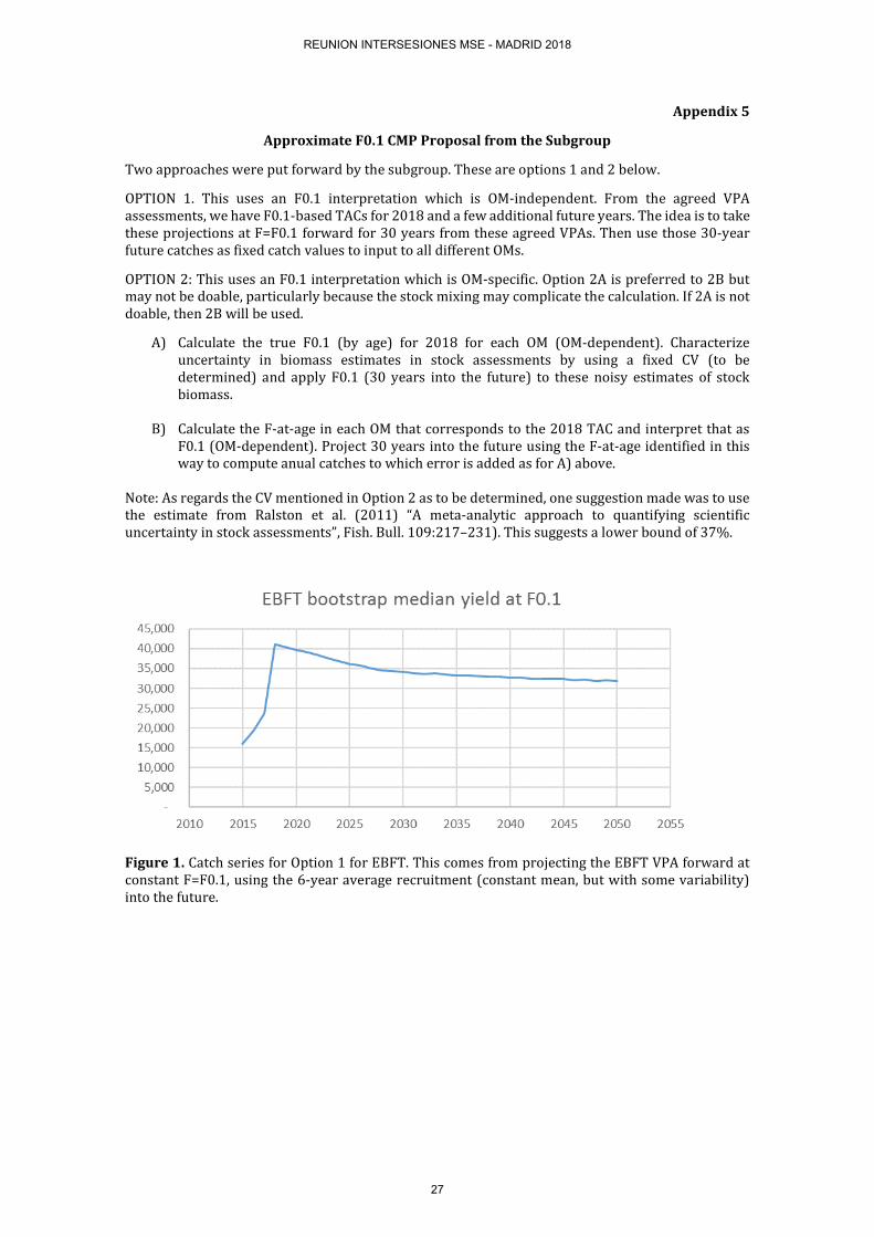
Appendix 5

Approximate F0.1 CMP Proposal from the Subgroup

Two approaches were put forward by the subgroup. These are options 1 and 2 below.

OPTION 1. This uses an F0.1 interpretation which is OM-independent. From the agreed VPA assessments, we have F0.1-based TACs for 2018 and a few additional future years. The idea is to take these projections at F=F0.1 forward for 30 years from these agreed VPAs. Then use those 30-year future catches as fixed catch values to input to all different OMs.

OPTION 2: This uses an F0.1 interpretation which is OM-specific. Option 2A is preferred to 2B but may not be doable, particularly because the stock mixing may complicate the calculation. If 2A is not doable, then 2B will be used.

A) Calculate the true F0.1 (by age) for 2018 for each OM (OM-dependent). Characterize uncertainty in biomass estimates in stock assessments by using a fixed CV (to be determined) and apply F0.1 (30 years into the future) to these noisy estimates of stock biomass.

B) Calculate the F-at-age in each OM that corresponds to the 2018 TAC and interpret that as F0.1 (OM-dependent). Project 30 years into the future using the F-at-age identified in this way to compute anual catches to which error is added as for A) above.

Note: As regards the CV mentioned in Option 2 as to be determined, one suggestion made was to use the estimate from Ralston et al. (2011) “A meta-analytic approach to quantifying scientific uncertainty in stock assessments”, Fish. Bull. 109:217–231). This suggests a lower bound of 37%.

Figure 1. Catch series for Option 1 for EBFT. This comes from projecting the EBFT VPA forward at constant F=F0.1, using the 6-year average recruitment (constant mean, but with some variability) into the future.


27

Appendix 6

Technical details of some of the CMPs

A. The DMM (Doug, Mitsuyo and Melissa) initial Candidate Management Procedure The DMM initial CMP is in essence a constant fishing mortality approach. It is applied separately to composite indices aggregated over those abundance indices available for each of the East and the West areas respectively. The control parameters setting this mortality may differ for the two areas, and each aggregate abundance index is averaged over the last three years for which data would be available so as to reduce variability in the index and consequently in TACs. TACs for each area are restricted not to change by more than 20% when the TAC is revised every second year. Details are provided below. Aggregate abundance indices An aggregate abundance index is developed for each of the East and the West areas by first standardising each index available for that area to an average value of 1 over the past years for which the index appeared reasonably stable1, and then taking a weighted average of the results for each index, where the weight is inversely proportional to the variance (𝜎𝜎2) shown by that standardised index over the chosen years. The mathematical details are as follows. 𝐽𝐽𝑦𝑦 is an average index over n series (n=4 for the East area and n=3 for the West area)

𝐽𝐽𝑦𝑦 =∑ 𝑤𝑤𝑖𝑖×𝐼𝐼𝑦𝑦𝑖𝑖∗𝑛𝑛𝑖𝑖∑ 𝑤𝑤𝑖𝑖𝑛𝑛𝑖𝑖

(1)

where 𝑤𝑤𝑖𝑖 = 1

�𝜎𝜎𝑖𝑖�2

and where the standardised index for each index series (i) is:

𝐼𝐼𝑦𝑦𝑖𝑖∗ = 𝐼𝐼𝑦𝑦𝑖𝑖𝐴𝐴𝐴𝐴𝐴𝐴𝐴𝐴𝐴𝐴𝐴𝐴𝐴𝐴 𝑜𝑜𝑜𝑜 ℎ𝑖𝑖𝑖𝑖𝑖𝑖𝑜𝑜𝐴𝐴𝑖𝑖𝑖𝑖𝐴𝐴𝑖𝑖 𝐼𝐼𝑦𝑦𝑖𝑖�

The actual index used in the CMPs, Jav, is the average over the last three years for which data would be available at the time the MP would be applied, hence2:

𝐽𝐽𝑎𝑎𝑎𝑎,𝑦𝑦 = 1

3�𝐽𝐽𝑦𝑦−2 + 𝐽𝐽𝑦𝑦−3 + 𝐽𝐽𝑦𝑦−4� (2)

where the J applies to either to the East or to the West area3.

CMP specifications The CMP sets the TAC every second year simply as a multiple of the Jav value for the area at the time, but subject to the change in the TAC for each area being restricted to a maximum of 20% (up or down). The formulae are given below. For the East area:

𝑇𝑇𝐴𝐴𝑇𝑇𝐸𝐸,𝑦𝑦 = �𝑇𝑇𝑇𝑇𝑇𝑇𝐸𝐸,2018𝐽𝐽𝐸𝐸,2016

� ∙ 𝛼𝛼 ∙ 𝐽𝐽𝑎𝑎𝑎𝑎,𝑦𝑦−2𝐸𝐸 4 (3a)

If 𝑇𝑇𝐴𝐴𝑇𝑇𝐸𝐸,𝑦𝑦≥1.2 ∗ 𝑇𝑇𝐴𝐴𝑇𝑇𝐸𝐸,𝑦𝑦−1 then 𝑇𝑇𝐴𝐴𝑇𝑇𝐸𝐸,𝑦𝑦 = 1.2 ∗ 𝑇𝑇𝐴𝐴𝑇𝑇𝐸𝐸,𝑦𝑦−1

1 These years commence from 2012 (JPN_LL_NEAtl2), 2010 for FR_AER_SUV, 2013 for MED_LAR_SUV, 2011 for MED_AER_SUV and JPN_LL2, 1994 for US_RR_115_144, and 1984 for GOM_LAR_SUV. 2 For the French and Mediterranean aerial survey, there is no value for 2014 and 2015 respectively. These years are omitted from this averaging where relevant. 3 The reason that the subscript on Jav is y-2 here is that one would set a TAC for year y during year y-1, at which time the most recent abundance indices available would be for year y-2.


28

If 𝑇𝑇𝐴𝐴𝑇𝑇𝐸𝐸,𝑦𝑦≤0.8 ∗ 𝑇𝑇𝐴𝐴𝑇𝑇𝐸𝐸,𝑦𝑦−1 then 𝑇𝑇𝐴𝐴𝑇𝑇𝐸𝐸,𝑦𝑦 = 0.8 ∗ 𝑇𝑇𝐴𝐴𝑇𝑇𝐸𝐸,𝑦𝑦−1

For the West area:

𝑇𝑇𝐴𝐴𝑇𝑇𝑊𝑊,𝑦𝑦 = �𝑇𝑇𝑇𝑇𝑇𝑇𝑊𝑊,2018𝐽𝐽𝑊𝑊,2016

� ∙ 𝛽𝛽 ∙ 𝐽𝐽𝑎𝑎𝑎𝑎,𝑦𝑦−2𝑊𝑊 (3b)

If 𝑇𝑇𝐴𝐴𝑇𝑇𝑊𝑊,𝑦𝑦≥1.2 ∗ 𝑇𝑇𝐴𝐴𝑇𝑇𝑊𝑊,𝑦𝑦−1 then 𝑇𝑇𝐴𝐴𝑇𝑇𝑊𝑊,𝑦𝑦 = 1.2 ∗ 𝑇𝑇𝐴𝐴𝑇𝑇𝑊𝑊,𝑦𝑦−1

If 𝑇𝑇𝐴𝐴𝑇𝑇𝑊𝑊,𝑦𝑦≤0.8 ∗ 𝑇𝑇𝐴𝐴𝑇𝑇𝑊𝑊,𝑦𝑦−1 then 𝑇𝑇𝐴𝐴𝑇𝑇𝑊𝑊,𝑦𝑦 = 0.8 ∗ 𝑇𝑇𝐴𝐴𝑇𝑇𝑊𝑊,𝑦𝑦−1

B. The DFO Candidate Management Procedure

A.R. Hanke

The DFO western MP (DFO7_40_10) uses index 7 (GOM_LAR_SUV) to predict stock status and derive a TAC recommendation. Healthy, cautious, critical and super critical zones are defined by the reference values 1.0, 0.4 and 0.1. The stock status at the conclusion of a management cycle is determined by comparing the ratio of the index value at the end of a cycle to a base value of the index. The base value is the mean of the index values in the last 3 years of the historical period.

In addition to an evaluation of status based on the index, the MP also determines the trend in the index over the most recent 4 years in order. The magnitude and direction of the trend affects the TAC recommendation conditional on stock status and comprise the control rules.

These control rules are as follows:

1. When the stock is in the healthy zone and the trend is positive, the TAC is increased by a scalar of 0.3 applied to the magnitude of the trend. Thus a slope of 1.0 increases the TAC by 30%. Otherwise, if the trend is negative there is no adjustment in the TAC.

2. When the stock is in the cautious zone and the trend is negative, the TAC is decreased by a scalar of 0.1 applied to the magnitude of the trend. Thus a slope of -1.0 decreases the TAC by 10%. Otherwise, if the trend is positive there is no adjustment in the TAC.

3. When the stock is in the critical zone, the TAC is decreased by a scalar of 0.1 applied to the magnitude of the trend 50%. In the event that the status falls below the critical zone, the TAC is set to 0.

In mathematical terms the MP works as follows:

𝐼𝐼𝑏𝑏𝑎𝑎𝑏𝑏𝑏𝑏 = � 𝐼𝐼𝑦𝑦 4⁄2015

𝑦𝑦=2012

𝐼𝐼𝑟𝑟𝑎𝑎𝑟𝑟𝑖𝑖𝑟𝑟 = 𝐼𝐼𝑛𝑛 𝐼𝐼𝑏𝑏𝑎𝑎𝑏𝑏𝑏𝑏⁄

𝛽𝛽 = 𝐼𝐼𝑗𝑗 − 𝛼𝛼 𝑌𝑌𝑗𝑗 , 𝑗𝑗 = 𝑦𝑦𝑛𝑛−3, … ,𝑦𝑦𝑛𝑛⁄

Healthy Zone

𝐼𝐼𝑟𝑟𝑎𝑎𝑟𝑟𝑖𝑖𝑟𝑟 ≥ 1 ∧ 𝛽𝛽 ≥ 0, 𝑇𝑇𝐴𝐴𝑇𝑇𝑦𝑦𝑛𝑛+1 = (1 + 𝛽𝛽 × 0.3) × 𝑇𝑇𝐴𝐴𝑇𝑇𝑦𝑦𝑛𝑛

𝐼𝐼𝑟𝑟𝑎𝑎𝑟𝑟𝑖𝑖𝑟𝑟 ≥ 1 ∧ 𝛽𝛽 < 0, 𝑇𝑇𝐴𝐴𝑇𝑇𝑦𝑦𝑛𝑛+1 = 𝑇𝑇𝐴𝐴𝑇𝑇𝑦𝑦𝑛𝑛

Cautious Zone

𝐼𝐼𝑟𝑟𝑎𝑎𝑟𝑟𝑖𝑖𝑟𝑟 < 1 ∧ 𝐼𝐼𝑟𝑟𝑎𝑎𝑟𝑟𝑖𝑖𝑟𝑟 ≥ 0.4 ∧ 𝛽𝛽 < 0, 𝑇𝑇𝐴𝐴𝑇𝑇𝑦𝑦𝑛𝑛+1 = (1 + 𝛽𝛽 × 0.1) × 𝑇𝑇𝐴𝐴𝑇𝑇𝑦𝑦𝑛𝑛


29

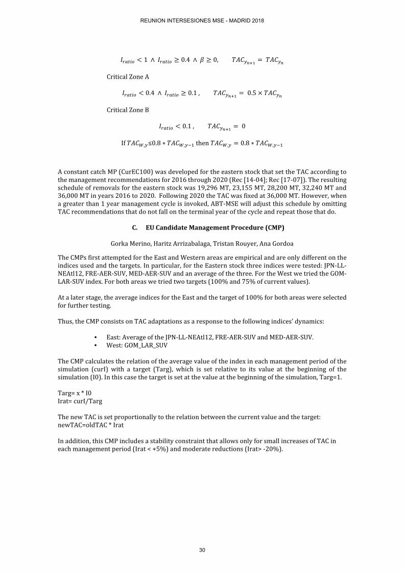
𝐼𝐼𝑟𝑟𝑎𝑎𝑟𝑟𝑖𝑖𝑟𝑟 < 1 ∧ 𝐼𝐼𝑟𝑟𝑎𝑎𝑟𝑟𝑖𝑖𝑟𝑟 ≥ 0.4 ∧ 𝛽𝛽 ≥ 0, 𝑇𝑇𝐴𝐴𝑇𝑇𝑦𝑦𝑛𝑛+1 = 𝑇𝑇𝐴𝐴𝑇𝑇𝑦𝑦𝑛𝑛

Critical Zone A

𝐼𝐼𝑟𝑟𝑎𝑎𝑟𝑟𝑖𝑖𝑟𝑟 < 0.4 ∧ 𝐼𝐼𝑟𝑟𝑎𝑎𝑟𝑟𝑖𝑖𝑟𝑟 ≥ 0.1 , 𝑇𝑇𝐴𝐴𝑇𝑇𝑦𝑦𝑛𝑛+1 = 0.5 × 𝑇𝑇𝐴𝐴𝑇𝑇𝑦𝑦𝑛𝑛

Critical Zone B

𝐼𝐼𝑟𝑟𝑎𝑎𝑟𝑟𝑖𝑖𝑟𝑟 < 0.1 , 𝑇𝑇𝐴𝐴𝑇𝑇𝑦𝑦𝑛𝑛+1 = 0

If 𝑇𝑇𝐴𝐴𝑇𝑇𝑊𝑊,𝑦𝑦≤0.8 ∗ 𝑇𝑇𝐴𝐴𝑇𝑇𝑊𝑊,𝑦𝑦−1 then 𝑇𝑇𝐴𝐴𝑇𝑇𝑊𝑊,𝑦𝑦 = 0.8 ∗ 𝑇𝑇𝐴𝐴𝑇𝑇𝑊𝑊,𝑦𝑦−1

A constant catch MP (CurEC100) was developed for the eastern stock that set the TAC according to the management recommendations for 2016 through 2020 (Rec [14-04]; Rec [17-07]). The resulting schedule of removals for the eastern stock was 19,296 MT, 23,155 MT, 28,200 MT, 32,240 MT and 36,000 MT in years 2016 to 2020. Following 2020 the TAC was fixed at 36,000 MT. However, when a greater than 1 year management cycle is invoked, ABT-MSE will adjust this schedule by omitting TAC recommendations that do not fall on the terminal year of the cycle and repeat those that do.

C. EU Candidate Management Procedure (CMP)

Gorka Merino, Haritz Arrizabalaga, Tristan Rouyer, Ana Gordoa

The CMPs first attempted for the East and Western areas are empirical and are only different on the indices used and the targets. In particular, for the Eastern stock three indices were tested: JPN-LL-NEAtl12, FRE-AER-SUV, MED-AER-SUV and an average of the three. For the West we tried the GOM-LAR-SUV index. For both areas we tried two targets (100% and 75% of current values). At a later stage, the average indices for the East and the target of 100% for both areas were selected for further testing. Thus, the CMP consists on TAC adaptations as a response to the following indices’ dynamics:

• East: Average of the JPN-LL-NEAtl12, FRE-AER-SUV and MED-AER-SUV. • West: GOM_LAR_SUV

The CMP calculates the relation of the average value of the index in each management period of the simulation (curI) with a target (Targ), which is set relative to its value at the beginning of the simulation (I0). In this case the target is set at the value at the beginning of the simulation, Targ=1. Targ= x * I0 Irat= curI/Targ The new TAC is set proportionally to the relation between the current value and the target: newTAC=oldTAC * Irat In addition, this CMP includes a stability constraint that allows only for small increases of TAC in each management period (Irat < +5%) and moderate reductions (Irat> -20%).


30

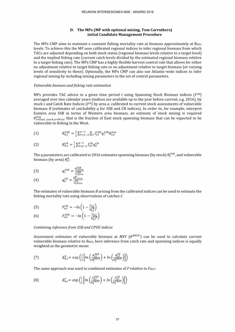
D. The MPx (MP with optional mixing, Tom Carruthers) initial Candidate Management Procedure

The MPx CMP aims to maintain a constant fishing mortality rate at biomass approximately at BMSY levels. To achieve this the MP uses calibrated regional indices to infer regional biomass from which TACs are adjusted depending on both stock status (regional biomass levels relative to a target level) and the implied fishing rate (current catch levels divided by the estimated regional biomass relative to a target fishing rate). The MPx CMP has a highly flexible harvest control rule that allows for either no adjustment relative to target fishing rate or no adjustment relative to target biomass (or varying levels of sensitivity to these). Optionally, the MPx CMP can also use Atlantic-wide indices to infer regional mixing by including mixing parameters in the set of control parameters. Vulnerable biomass and fishing rate estimation MPx provides TAC advice in a given time period t using Spawning Stock Biomass indices (ISSB) averaged over two calendar years (indices are available up to the year before current, e.g. 2016), by stock s and Catch Rate Indices (ICR) by area a, calibrated to current stock assessments of vulnerable biomass B (estimates of catchability q for SSB and CR indices). In order to, for example, interpret Eastern area SSB in terms of Western area biomass, an estimate of stock mixing is required 𝜃𝜃𝑏𝑏=𝐸𝐸𝑎𝑎𝑏𝑏𝑟𝑟_𝑏𝑏𝑟𝑟𝑟𝑟𝑠𝑠𝑠𝑠,𝑎𝑎=𝑊𝑊𝑏𝑏𝑏𝑏𝑟𝑟𝑚𝑚𝑖𝑖𝑚𝑚 that is the fraction of East stock spawning biomass that can be expected to be

vulnerable to fishing in the West. (1) 𝐵𝐵𝑎𝑎,𝑟𝑟

𝑆𝑆𝑆𝑆𝑆𝑆 = 12∑ ∑ 𝐼𝐼𝑏𝑏,𝑟𝑟

𝑆𝑆𝑆𝑆𝑆𝑆𝑞𝑞𝑏𝑏𝑆𝑆𝑆𝑆𝑆𝑆𝜃𝜃𝑏𝑏,𝑎𝑎𝑚𝑚𝑖𝑖𝑚𝑚

𝑏𝑏𝑦𝑦−1𝑟𝑟=𝑦𝑦−2

(2) 𝐵𝐵𝑎𝑎,𝑟𝑟

𝑇𝑇𝐶𝐶 = 12∑ 𝐼𝐼𝑎𝑎,𝑟𝑟

𝑇𝑇𝐶𝐶𝑞𝑞𝑎𝑎𝑇𝑇𝐶𝐶y−1t=y−2

The q parameters are calibrated to 2016 estimates spawning biomass (by stock) 𝜃𝜃𝑏𝑏𝑆𝑆𝑆𝑆𝑆𝑆 , and vulnerable biomass (by area) 𝜃𝜃𝑎𝑎𝑆𝑆:

(3) 𝑞𝑞𝑏𝑏𝑆𝑆𝑆𝑆𝑆𝑆 = 𝜃𝜃𝑠𝑠,2016𝑆𝑆𝑆𝑆𝑆𝑆

𝐼𝐼𝑠𝑠,2016𝑆𝑆𝑆𝑆𝑆𝑆

(4) 𝑞𝑞𝑎𝑎𝑇𝑇𝐶𝐶 = 𝜃𝜃𝑎𝑎,2016𝑆𝑆

𝐼𝐼𝑎𝑎,2016𝐶𝐶𝐶𝐶

The estimates of vulnerable biomass B arising from the calibrated indices can be used to estimate the fishing mortality rate using observations of catches C (5) 𝐹𝐹𝑎𝑎,𝑟𝑟

𝑇𝑇𝐶𝐶 = −ln �1 − 𝑇𝑇𝑎𝑎,𝑡𝑡𝑆𝑆𝑎𝑎,𝑡𝑡𝐶𝐶𝐶𝐶�

(6) 𝐹𝐹𝑎𝑎,𝑟𝑟𝑆𝑆𝑆𝑆𝑆𝑆 = −ln �1 − 𝑇𝑇𝑎𝑎,𝑡𝑡

𝑆𝑆𝑎𝑎,𝑡𝑡𝑆𝑆𝑆𝑆𝑆𝑆�

Combining inference from SSB and CPUE indices Assessment estimates of vulnerable biomass at MSY (𝜃𝜃𝑆𝑆𝐵𝐵𝑆𝑆𝐵𝐵) can be used to calculate current vulnerable biomass relative to BMSY, here inference from catch rate and spawning indices is equally weighted as the geometric mean:

(7) ∆𝑎𝑎,𝑟𝑟𝑆𝑆 = 𝐴𝐴𝑒𝑒𝑒𝑒 �1

2�𝑖𝑖𝑙𝑙 � 𝑆𝑆𝑎𝑎,𝑡𝑡

𝑆𝑆𝑆𝑆𝑆𝑆

𝜃𝜃𝑎𝑎𝑆𝑆𝐵𝐵𝑆𝑆𝐵𝐵� + 𝑖𝑖𝑙𝑙 � 𝑆𝑆𝑎𝑎,𝑡𝑡𝐶𝐶𝐶𝐶

𝜃𝜃𝑎𝑎𝑆𝑆𝐵𝐵𝑆𝑆𝐵𝐵�� The same approach was used to combined estimates of F relative to FMSY:

(8) ∆𝑎𝑎,𝑟𝑟𝐹𝐹 = exp �1

2�𝑖𝑖𝑙𝑙 � 𝐹𝐹𝑎𝑎,𝑡𝑡

𝑆𝑆𝑆𝑆𝑆𝑆

𝜃𝜃𝑎𝑎𝐹𝐹𝐵𝐵𝑆𝑆𝐵𝐵� + 𝑖𝑖𝑙𝑙 � 𝐹𝐹𝑎𝑎,𝑡𝑡𝐶𝐶𝐶𝐶

𝜃𝜃𝑎𝑎𝐹𝐹𝐵𝐵𝑆𝑆𝐵𝐵��


31

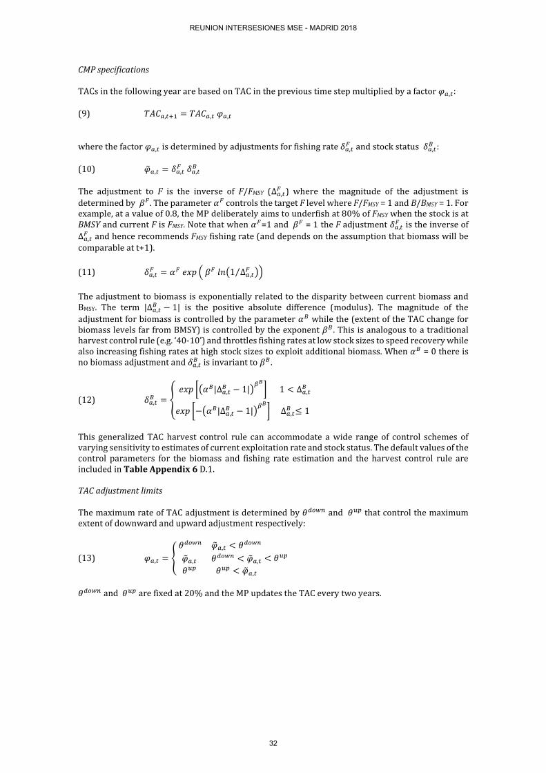
CMP specifications TACs in the following year are based on TAC in the previous time step multiplied by a factor 𝜑𝜑𝑎𝑎,𝑟𝑟: (9) 𝑇𝑇𝐴𝐴𝑇𝑇𝑎𝑎,𝑟𝑟+1 = 𝑇𝑇𝐴𝐴𝑇𝑇𝑎𝑎,𝑟𝑟 𝜑𝜑𝑎𝑎,𝑟𝑟 where the factor 𝜑𝜑𝑎𝑎,𝑟𝑟 is determined by adjustments for fishing rate 𝛿𝛿𝑎𝑎,𝑟𝑟

𝐹𝐹 and stock status 𝛿𝛿𝑎𝑎,𝑟𝑟𝑆𝑆 :

(10) 𝜑𝜑�𝑎𝑎,𝑟𝑟 = 𝛿𝛿𝑎𝑎,𝑟𝑟

𝐹𝐹 𝛿𝛿𝑎𝑎,𝑟𝑟𝑆𝑆

The adjustment to F is the inverse of F/FMSY (∆𝑎𝑎,𝑟𝑟

𝐹𝐹 ) where the magnitude of the adjustment is determined by 𝛽𝛽𝐹𝐹. The parameter 𝛼𝛼𝐹𝐹 controls the target F level where F/FMSY = 1 and B/BMSY = 1. For example, at a value of 0.8, the MP deliberately aims to underfish at 80% of FMSY when the stock is at BMSY and current F is FMSY. Note that when 𝛼𝛼𝐹𝐹=1 and 𝛽𝛽𝐹𝐹 = 1 the F adjustment 𝛿𝛿𝑎𝑎,𝑟𝑟

𝐹𝐹 is the inverse of ∆𝑎𝑎,𝑟𝑟𝐹𝐹 and hence recommends FMSY fishing rate (and depends on the assumption that biomass will be

comparable at t+1). (11) 𝛿𝛿𝑎𝑎,𝑟𝑟

𝐹𝐹 = 𝛼𝛼𝐹𝐹 𝐴𝐴𝑒𝑒𝑒𝑒 � 𝛽𝛽𝐹𝐹 𝑖𝑖𝑙𝑙�1 ∆𝑎𝑎,𝑟𝑟𝐹𝐹⁄ ��

The adjustment to biomass is exponentially related to the disparity between current biomass and BMSY. The term |∆𝑎𝑎,𝑟𝑟

𝑆𝑆 − 1| is the positive absolute difference (modulus). The magnitude of the adjustment for biomass is controlled by the parameter 𝛼𝛼𝑆𝑆 while the (extent of the TAC change for biomass levels far from BMSY) is controlled by the exponent 𝛽𝛽𝑆𝑆 . This is analogous to a traditional harvest control rule (e.g. ‘40-10’) and throttles fishing rates at low stock sizes to speed recovery while also increasing fishing rates at high stock sizes to exploit additional biomass. When 𝛼𝛼𝑆𝑆 = 0 there is no biomass adjustment and 𝛿𝛿𝑎𝑎,𝑟𝑟

𝑆𝑆 is invariant to 𝛽𝛽𝑆𝑆 .

(12) 𝛿𝛿𝑎𝑎,𝑟𝑟𝑆𝑆 = �

𝐴𝐴𝑒𝑒𝑒𝑒 ��𝛼𝛼𝑆𝑆|∆𝑎𝑎,𝑟𝑟𝑆𝑆 − 1|�𝛽𝛽

𝑆𝑆� 1 < ∆𝑎𝑎,𝑟𝑟

𝑆𝑆

𝐴𝐴𝑒𝑒𝑒𝑒 �−�𝛼𝛼𝑆𝑆|∆𝑎𝑎,𝑟𝑟𝑆𝑆 − 1|�𝛽𝛽

𝑆𝑆� ∆𝑎𝑎,𝑟𝑟

𝑆𝑆 ≤ 1

This generalized TAC harvest control rule can accommodate a wide range of control schemes of varying sensitivity to estimates of current exploitation rate and stock status. The default values of the control parameters for the biomass and fishing rate estimation and the harvest control rule are included in Table Appendix 6 D.1. TAC adjustment limits The maximum rate of TAC adjustment is determined by 𝜃𝜃𝑑𝑑𝑟𝑟𝑤𝑤𝑛𝑛 and 𝜃𝜃𝑢𝑢𝑢𝑢 that control the maximum extent of downward and upward adjustment respectively:

(13) 𝜑𝜑𝑎𝑎,𝑟𝑟 = � 𝜃𝜃𝑑𝑑𝑟𝑟𝑤𝑤𝑛𝑛 𝜑𝜑�𝑎𝑎,𝑟𝑟 < 𝜃𝜃𝑑𝑑𝑟𝑟𝑤𝑤𝑛𝑛

𝜑𝜑�𝑎𝑎,𝑟𝑟 𝜃𝜃𝑑𝑑𝑟𝑟𝑤𝑤𝑛𝑛 < 𝜑𝜑�𝑎𝑎,𝑟𝑟 𝜃𝜃𝑢𝑢𝑢𝑢 𝜃𝜃𝑢𝑢𝑢𝑢 < 𝜑𝜑�𝑎𝑎,𝑟𝑟

< 𝜃𝜃𝑢𝑢𝑢𝑢

𝜃𝜃𝑑𝑑𝑟𝑟𝑤𝑤𝑛𝑛 and 𝜃𝜃𝑢𝑢𝑢𝑢 are fixed at 20% and the MP updates the TAC every two years.


32

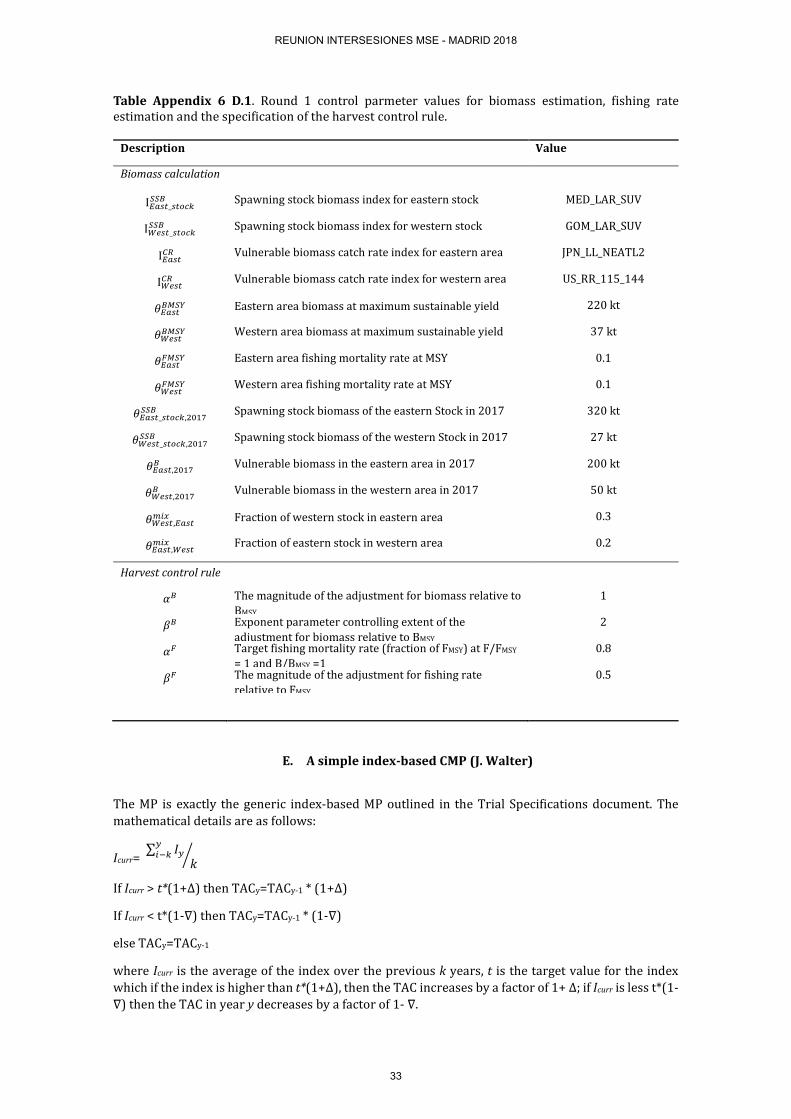
Table Appendix 6 D.1. Round 1 control parmeter values for biomass estimation, fishing rate estimation and the specification of the harvest control rule.

Description Value

Biomass calculation

I𝐸𝐸𝑎𝑎𝑏𝑏𝑟𝑟_𝑏𝑏𝑟𝑟𝑟𝑟𝑠𝑠𝑠𝑠𝑆𝑆𝑆𝑆𝑆𝑆 Spawning stock biomass index for eastern stock MED_LAR_SUV

I𝑊𝑊𝑏𝑏𝑏𝑏𝑟𝑟_𝑏𝑏𝑟𝑟𝑟𝑟𝑠𝑠𝑠𝑠𝑆𝑆𝑆𝑆𝑆𝑆 Spawning stock biomass index for western stock GOM_LAR_SUV

I𝐸𝐸𝑎𝑎𝑏𝑏𝑟𝑟𝑇𝑇𝐶𝐶 Vulnerable biomass catch rate index for eastern area JPN_LL_NEATL2

I𝑊𝑊𝑏𝑏𝑏𝑏𝑟𝑟𝑇𝑇𝐶𝐶 Vulnerable biomass catch rate index for western area US_RR_115_144

𝜃𝜃𝐸𝐸𝑎𝑎𝑏𝑏𝑟𝑟𝑆𝑆𝐵𝐵𝑆𝑆𝐵𝐵 Eastern area biomass at maximum sustainable yield 220 kt

𝜃𝜃𝑊𝑊𝑏𝑏𝑏𝑏𝑟𝑟𝑆𝑆𝐵𝐵𝑆𝑆𝐵𝐵 Western area biomass at maximum sustainable yield 37 kt

𝜃𝜃𝐸𝐸𝑎𝑎𝑏𝑏𝑟𝑟𝐹𝐹𝐵𝐵𝑆𝑆𝐵𝐵 Eastern area fishing mortality rate at MSY 0.1

𝜃𝜃𝑊𝑊𝑏𝑏𝑏𝑏𝑟𝑟𝐹𝐹𝐵𝐵𝑆𝑆𝐵𝐵 Western area fishing mortality rate at MSY 0.1

𝜃𝜃𝐸𝐸𝑎𝑎𝑏𝑏𝑟𝑟_𝑏𝑏𝑟𝑟𝑟𝑟𝑠𝑠𝑠𝑠,2017𝑆𝑆𝑆𝑆𝑆𝑆 Spawning stock biomass of the eastern Stock in 2017 320 kt

𝜃𝜃𝑊𝑊𝑏𝑏𝑏𝑏𝑟𝑟_𝑏𝑏𝑟𝑟𝑟𝑟𝑠𝑠𝑠𝑠,2017𝑆𝑆𝑆𝑆𝑆𝑆 Spawning stock biomass of the western Stock in 2017 27 kt

𝜃𝜃𝐸𝐸𝑎𝑎𝑏𝑏𝑟𝑟,2017𝑆𝑆 Vulnerable biomass in the eastern area in 2017 200 kt

𝜃𝜃𝑊𝑊𝑏𝑏𝑏𝑏𝑟𝑟,2017𝑆𝑆 Vulnerable biomass in the western area in 2017 50 kt

𝜃𝜃𝑊𝑊𝑏𝑏𝑏𝑏𝑟𝑟,𝐸𝐸𝑎𝑎𝑏𝑏𝑟𝑟𝑚𝑚𝑖𝑖𝑚𝑚 Fraction of western stock in eastern area 0.3

𝜃𝜃𝐸𝐸𝑎𝑎𝑏𝑏𝑟𝑟,𝑊𝑊𝑏𝑏𝑏𝑏𝑟𝑟𝑚𝑚𝑖𝑖𝑚𝑚 Fraction of eastern stock in western area 0.2

Harvest control rule

𝛼𝛼𝑆𝑆 The magnitude of the adjustment for biomass relative to BMSY

1

𝛽𝛽𝑆𝑆 Exponent parameter controlling extent of the adjustment for biomass relative to BMSY

2

𝛼𝛼𝐹𝐹 Target fishing mortality rate (fraction of FMSY) at F/FMSY = 1 and B/BMSY =1

0.8

𝛽𝛽𝐹𝐹 The magnitude of the adjustment for fishing rate relative to FMSY

0.5

E. A simple index-based CMP (J. Walter)

The MP is exactly the generic index-based MP outlined in the Trial Specifications document. The mathematical details are as follows:

Icurr= ∑ 𝐼𝐼𝑦𝑦𝑦𝑦𝑖𝑖−𝑠𝑠

𝑘𝑘�

If Icurr > t*(1+∆) then TACy=TACy-1 * (1+∆)

If Icurr < t*(1-∇) then TACy=TACy-1 * (1-∇)

else TACy=TACy-1

where Icurr is the average of the index over the previous k years, t is the target value for the index which if the index is higher than t*(1+∆), then the TAC increases by a factor of 1+ ∆; if Icurr is less t*(1-∇) then the TAC in year y decreases by a factor of 1- ∇.


33

To apply this to an index it is necessary to define the index and the control parameters of the target value, the percentage increase and the percentage decrease and the number of years over which to average the index. A USRR 115_144 index CMP for East and West areas A candidate management procedure (CMP) based on the USRR 115_144 index for both East and West areas. It alters the current TAC according to the ratio of the index averaged over k years relative to the chosen target value of the index. The concept of using this index for both East and West areas comes from the observation that this index is for ages 4 and 5 year old fish, which are of mixed Eastern and Western origin in the fishery that this index comes from. Hence this index is the first index to see recruits from both stocks and may be useful for tracking recruitment. The CMP exactly follows the example MP in the trial specification document. As such it is it not expressly particularly designed for good performance and further MP development may change control parameter settings or the actual design of any CMP that uses the USRR 115_144 index. To create an MP based on the USRR 115_144 index (index 6) as the single index for both East and Western areas we specified the ∆ as 0.05 and ∇ as 0.2. Two years were chosen to average the index (k=2) and several different values for the target were explored from 0.25-0.8.


34

Appendix 7

SPECIFICATIONS FOR MSE TRIALS FOR BLUEFIN TUNA IN THE NORTH ATLANTIC

CONTENTS 1. BASIC CONCEPTS AND STOCK STRUCTURE ............................................ 35

I) Spatial strata ................................................................................................................................... 35 Baseline ......................................................................................................................................... 35 Alternative low priority future options .......................................................................................... 35

II) Stock mixing ................................................................................................................................. 36 Baseline ......................................................................................................................................... 36 Possible alternative options ........................................................................................................... 36

2. PAST DATA AVAILABLE ............................................................................... 36 I) Raw data ........................................................................................................................................ 37 II) Analysed data ............................................................................................................................... 37 III) Assumptions ................................................................................................................................ 40

3. BASIC DYNAMICS ........................................................................................... 45 I) Overview ........................................................................................................................................ 45 II) Equations ...................................................................................................................................... 45

Baseline ......................................................................................................................................... 49 Alternative options ........................................................................................................................ 49

III) Fleet structure and exploitation history ....................................................................................... 50 Baseline ......................................................................................................................................... 50 Alternative options ........................................................................................................................ 50

4. MANAGEMENT OPTIONS .............................................................................. 50 I) Spatial strata for which TACs are set ............................................................................................. 51


II) Options for the frequency of setting TACs ................................................................................... 51 Baseline ......................................................................................................................................... 51 Alternative options ........................................................................................................................ 51

III) Upper limits on TACs ................................................................................................................. 51 IV) Minimum extent of TAC change ................................................................................................ 52


V) Maximum extent of TAC change ................................................................................................. 52 Baseline ......................................................................................................................................... 52 Alternative options ........................................................................................................................ 52

VI) Technical measures ..................................................................................................................... 52 5. FUTURE RECRUITMENT AND DISTRIBUTION SCENARIOS .................. 52

I) West ............................................................................................................................................... 53 II) East + Mediterranean .................................................................................................................... 53 III) Future regime shifts ..................................................................................................................... 53

West ............................................................................................................................................... 53 East+Med ...................................................................................................................................... 53

IV) Statistical properties .................................................................................................................... 53 Baseline ......................................................................................................................................... 53 Alternative options ........................................................................................................................ 54

V) Possible future distributional changes .......................................................................................... 54 6. FUTURE CATCHES .......................................................................................... 54


7. GENERATION OF FUTURE DATA ................................................................. 54 I) Baseline suggestions ...................................................................................................................... 55

West ............................................................................................................................................... 55 East+Med ...................................................................................................................................... 55

II) Alternative options........................................................................................................................ 55


35

III) Relationships with abundance ..................................................................................................... 55 IV) Statistical properties .................................................................................................................... 56


Other aspects ............................................................................................................................. 56 8. PARAMETERS AND CONDITIONING ........................................................... 57

I) Fixed parameters ............................................................................................................................ 57 II) Estimated parameters .................................................................................................................... 58 III) Characterising uncertainty ........................................................................................................... 64


9. TRIAL SPECIFICATIONS ................................................................................. 65 A. Reference set .................................................................................................................. 65 B. Robustness trials............................................................................................................. 66

10. PERFORMANCE MEASURES/STATISTICS .................................................. 66 I) Summary measures/statistics ......................................................................................................... 67 II) Summary plots .............................................................................................................................. 67 III) Level of reporting ........................................................................................................................ 68



36

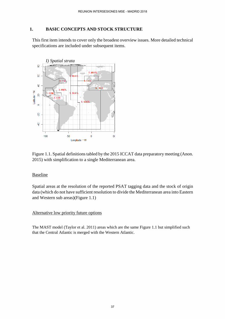
1. BASIC CONCEPTS AND STOCK STRUCTURE This first item intends to cover only the broadest overview issues. More detailed technical specifications are included under subsequent items.

I) Spatial strata

Figure 1.1. Spatial definitions tabled by the 2015 ICCAT data preparatory meeting (Anon. 2015) with simplification to a single Mediterranean area.

Baseline Spatial areas at the resolution of the reported PSAT tagging data and the stock of origin data (which do not have sufficient resolution to divide the Mediterranean area into Eastern and Western sub areas)(Figure 1.1)

Alternative low priority future options

The MAST model (Taylor et al. 2011) areas which are the same Figure 1.1 but simplified such that the Central Atlantic is merged with the Western Atlantic.


37

II) Stock mixing

Baseline A two-stock model similar to Figure 1.2A but adhering to the spatial structure of Figure 1.1A and including the mixing for West Africa which was discovered after the Tenerife meeting.

Possible alternative options A two-stock model with no mixing

2. PAST DATA AVAILABLE Table 2.1 provides an overview of the data that may be used to condition operating models for Atlantic bluefin tuna. The Table indicates those data that have been gathered, those that are currently available and those that have already been used in conditioning operating models.

Figure 1.2. Mixing hypotheses suggested by Arrizabalaga et al. 2014).

(A) A two stock model with no sub-populations.

(B) A two stock model with sub-population structure.

(C) A complex 2+ stock model.

A B

C


38

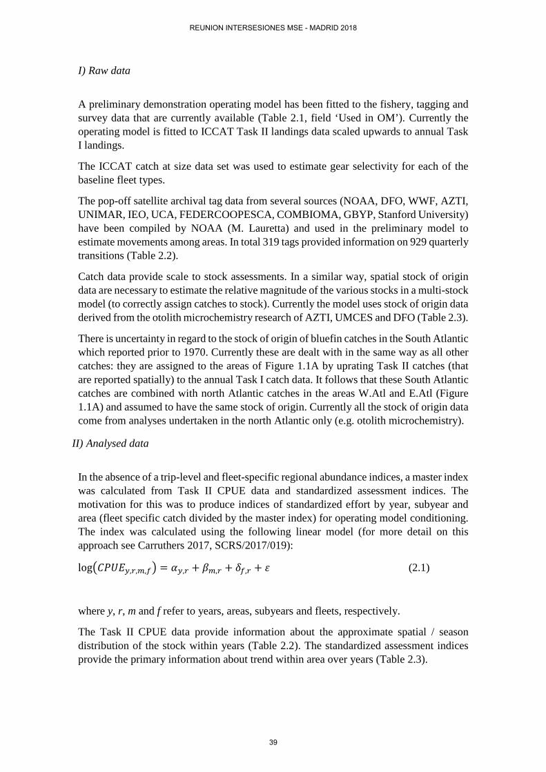
I) Raw data

A preliminary demonstration operating model has been fitted to the fishery, tagging and survey data that are currently available (Table 2.1, field ‘Used in OM’). Currently the operating model is fitted to ICCAT Task II landings data scaled upwards to annual Task I landings.

The ICCAT catch at size data set was used to estimate gear selectivity for each of the baseline fleet types.

The pop-off satellite archival tag data from several sources (NOAA, DFO, WWF, AZTI, UNIMAR, IEO, UCA, FEDERCOOPESCA, COMBIOMA, GBYP, Stanford University) have been compiled by NOAA (M. Lauretta) and used in the preliminary model to estimate movements among areas. In total 319 tags provided information on 929 quarterly transitions (Table 2.2).

Catch data provide scale to stock assessments. In a similar way, spatial stock of origin data are necessary to estimate the relative magnitude of the various stocks in a multi-stock model (to correctly assign catches to stock). Currently the model uses stock of origin data derived from the otolith microchemistry research of AZTI, UMCES and DFO (Table 2.3).

There is uncertainty in regard to the stock of origin of bluefin catches in the South Atlantic which reported prior to 1970. Currently these are dealt with in the same way as all other catches: they are assigned to the areas of Figure 1.1A by uprating Task II catches (that are reported spatially) to the annual Task I catch data. It follows that these South Atlantic catches are combined with north Atlantic catches in the areas W.Atl and E.Atl (Figure 1.1A) and assumed to have the same stock of origin. Currently all the stock of origin data come from analyses undertaken in the north Atlantic only (e.g. otolith microchemistry).

II) Analysed data

In the absence of a trip-level and fleet-specific regional abundance indices, a master index was calculated from Task II CPUE data and standardized assessment indices. The motivation for this was to produce indices of standardized effort by year, subyear and area (fleet specific catch divided by the master index) for operating model conditioning. The index was calculated using the following linear model (for more detail on this approach see Carruthers 2017, SCRS/2017/019):

log�𝐶𝐶𝐶𝐶𝐶𝐶𝐶𝐶𝑦𝑦,𝑟𝑟,𝑚𝑚,𝑓𝑓� = 𝛼𝛼𝑦𝑦,𝑟𝑟 + 𝛽𝛽𝑚𝑚,𝑟𝑟 + 𝛿𝛿𝑓𝑓,𝑟𝑟 + 𝜀𝜀 (2.1)

where y, r, m and f refer to years, areas, subyears and fleets, respectively.

The Task II CPUE data provide information about the approximate spatial / season distribution of the stock within years (Table 2.2). The standardized assessment indices provide the primary information about trend within area over years (Table 2.3).


39

Table 2.2. The Task II CPUE data used to derive the master index.

Flag Gear Details

Japan Longline 1.38m fish

USA Longline 13,156 fish

Canada Rod and reel 9,131 tonnes

Morocco Trap 15,996 tonnes

Spain Baitboat 35,625 tonnes

Table 2.3. The standardized CPUE indices of the assessments that are used to derive trend information for the master index and also fit the operating models.

Flag Gear Details

Spain Baitboat 1952-2006, Q3, E Atl

Spain / France Baitboat 2007-2014, Q3, E Atl

Morocco / Spain Trap 1981-2011, Q2, SE Atl

Morocco / Portugal Trap 2012-2016, Q2, SE Atl

Japan Longline 1975-2009, Q2, SE Atl

Japan Longline 1990-2009, Q4, NE Atl

Japan Longline 2010-2017, Q4, NE Atl

US (66cm - 114cm) Rod and reel 1993-2015, Q3, W Atl

US (115cm - 144cm) Rod and reel 1993-2015, Q3, W Atl

US (145cm +) Rod and reel 1980-1992, Q3, W Atl

US (195cm +) Rod and reel 1984-1992, Q3, W Atl

US Longline 1987-1991, Q2, GOM

US Longline 1992-2016, Q2, GOM

Japan Longline 1976-2009, Q4, W Atl

Japan Longline 2010-2017, Q4, W Atl

Canada Rod and reel 1984-2016, Q3, W Atl

Italy Trap 1993-2010, Q2, Med


40

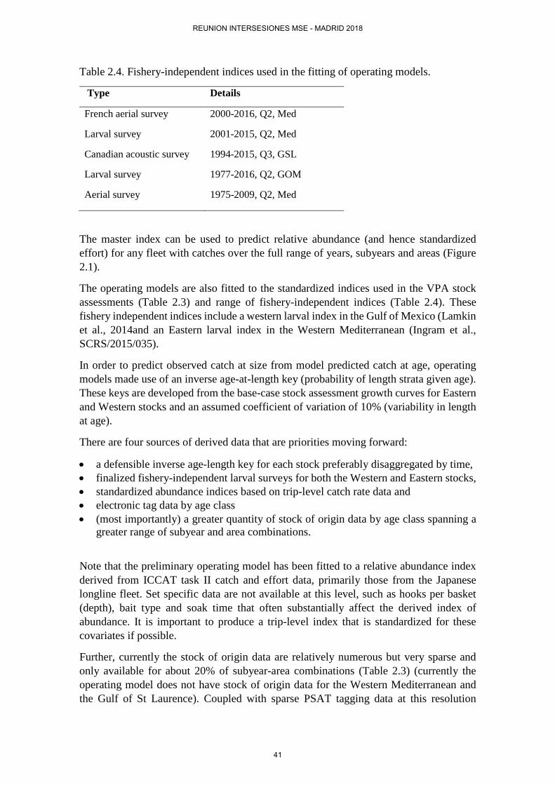
Table 2.4. Fishery-independent indices used in the fitting of operating models.

Type Details

French aerial survey 2000-2016, Q2, Med

Larval survey 2001-2015, Q2, Med

Canadian acoustic survey 1994-2015, Q3, GSL

Larval survey 1977-2016, Q2, GOM

Aerial survey 1975-2009, Q2, Med

The master index can be used to predict relative abundance (and hence standardized effort) for any fleet with catches over the full range of years, subyears and areas (Figure 2.1).

The operating models are also fitted to the standardized indices used in the VPA stock assessments (Table 2.3) and range of fishery-independent indices (Table 2.4). These fishery independent indices include a western larval index in the Gulf of Mexico (Lamkin et al., 2014and an Eastern larval index in the Western Mediterranean (Ingram et al., SCRS/2015/035).

In order to predict observed catch at size from model predicted catch at age, operating models made use of an inverse age-at-length key (probability of length strata given age). These keys are developed from the base-case stock assessment growth curves for Eastern and Western stocks and an assumed coefficient of variation of 10% (variability in length at age).

There are four sources of derived data that are priorities moving forward:

• a defensible inverse age-length key for each stock preferably disaggregated by time, • finalized fishery-independent larval surveys for both the Western and Eastern stocks, • standardized abundance indices based on trip-level catch rate data and • electronic tag data by age class • (most importantly) a greater quantity of stock of origin data by age class spanning a

greater range of subyear and area combinations.

Note that the preliminary operating model has been fitted to a relative abundance index derived from ICCAT task II catch and effort data, primarily those from the Japanese longline fleet. Set specific data are not available at this level, such as hooks per basket (depth), bait type and soak time that often substantially affect the derived index of abundance. It is important to produce a trip-level index that is standardized for these covariates if possible.

Further, currently the stock of origin data are relatively numerous but very sparse and only available for about 20% of subyear-area combinations (Table 2.3) (currently the operating model does not have stock of origin data for the Western Mediterranean and the Gulf of St Laurence). Coupled with sparse PSAT tagging data at this resolution


41

(Table 2.2), there is limited information to estimate age-specific movement and allow the model to apportion catches to stock in these time-area strata correctly. There are however a large number of studies that may provide estimates of the stock of origin the data of which are not currently used to condition the operating model (e.g. otolith microchemistry, SNP, otolith shape and mitochondrial DNA analyses). Along with additional electronic tagging data by age class, provision of these stock of origin data by age class is arguably the highest priority for successfully conditioning future operating models.

III) Assumptions The following are the default assumptions made in the model. Some of them may be relaxed in the robustness trials.

The age-length key is static and not adjusted according to fishing mortality rate and length selectivity of fishing.

CPUE indices are considered to be proportional to exploitable biomass (weighted by the selectivity indices).

Larval indices are assumed to be proportional to spawning stock biomass in the area in which they were collected in contrast to stock-wide spawning stock biomass (for scenarios where the two are not proportional).


42

Table 2.1. Overview of data that may be used to inform operating models for Atlantic bluefin tuna (available online here). Cells shaded green reflect sources for which data are available (‘Collab’,the Core modelling group CMG, or the ICCAT secretariat) and whether data that are available have also been used in conditioning preliminary operating models (‘used in OM?’)


43

https://drive.google.com/open?id=140HrddEWU_MFHhxizVtaO_uRs48tzPrEgbDMwudl_1M

Table 2.1 continued.


44

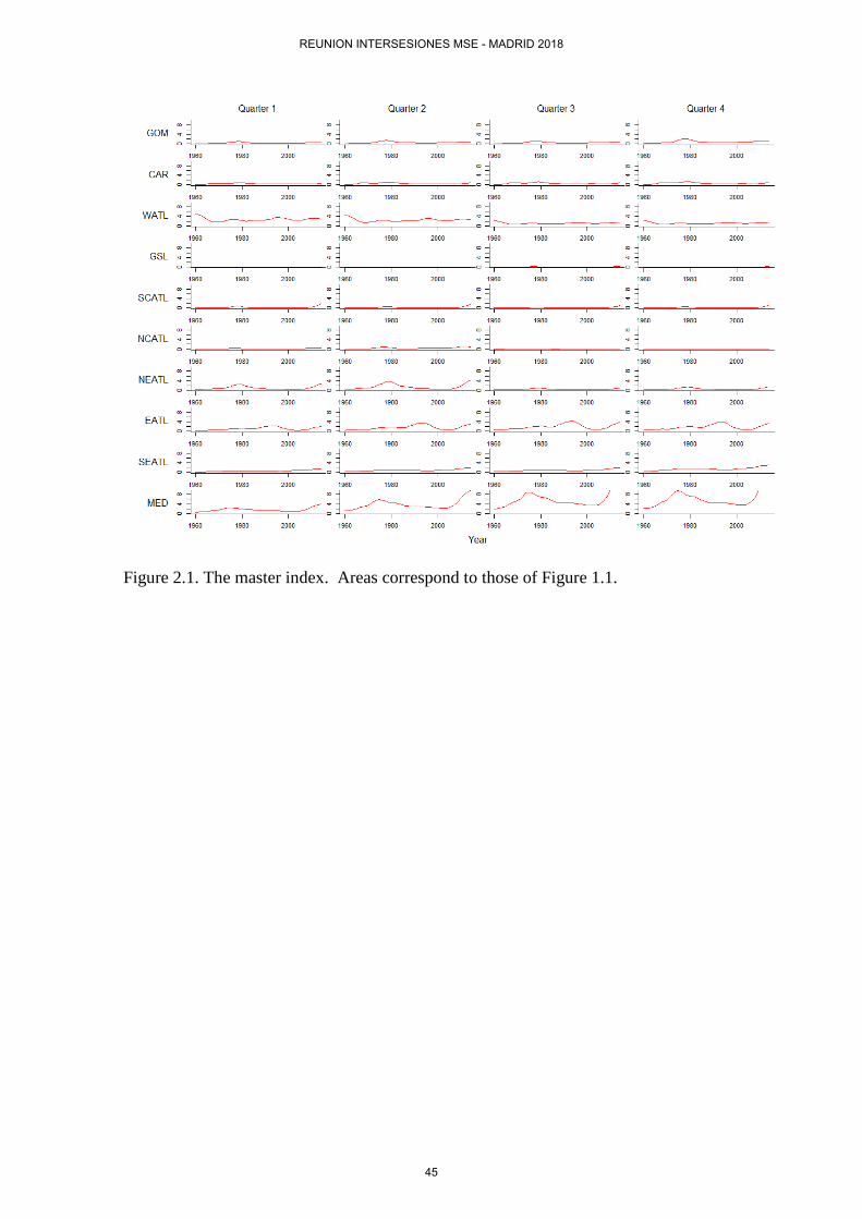
Figure 2.1. The master index. Areas correspond to those of Figure 1.1.


45

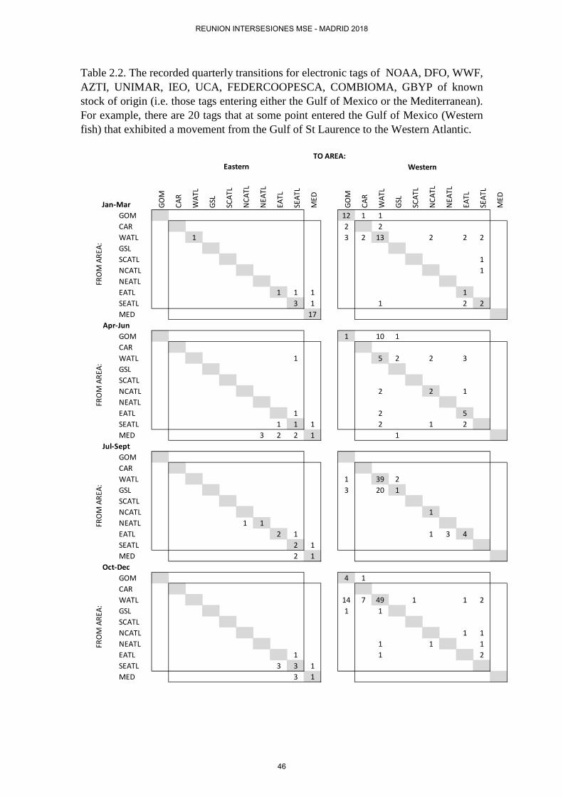
Table 2.2. The recorded quarterly transitions for electronic tags of NOAA, DFO, WWF, AZTI, UNIMAR, IEO, UCA, FEDERCOOPESCA, COMBIOMA, GBYP of known stock of origin (i.e. those tags entering either the Gulf of Mexico or the Mediterranean). For example, there are 20 tags that at some point entered the Gulf of Mexico (Western fish) that exhibited a movement from the Gulf of St Laurence to the Western Atlantic.

GOM

CAR

WAT

L

GSL

SCAT

L

NCA

TL

NEA

TL

EATL

SEAT

L

MED

GOM

CAR

WAT

L

GSL

SCAT

L

NCA

TL

NEA

TL

EATL

SEAT

L

MED

GOM NA NA NA NA NA NA NA NA NA 12 1 1 NA NA NA NA NA NA NACAR NA NA NA NA NA NA NA NA NA 2 2 NA NA NA NA NA NA NAWATL NA NA 1 NA NA NA NA NA NA NA 3 2 13 NA NA 2 NA 2 2GSL NA NA NA NA NA NA NA NA NA NA NA NA NA NA NA NA NA NASCATL NA NA NA NA NA NA NA NA NA NA NA NA NA NA NA NA 1 NANCATL NA NA NA NA NA NA NA NA NA NA NA NA NA NA NA NA 1 NANEATL NA NA NA NA NA NA NA NA NA NA NA NA NA NA NA NA NA NAEATL NA NA NA NA NA NA NA 1 1 1 NA NA NA NA NA NA NA 1 NA NASEATL NA NA NA NA NA NA NA NA 3 1 NA NA 1 NA NA NA NA 2 2 NAMED NA NA NA NA NA NA NA NA NA 17 NA NA NA NA NA NA NA NA NA

GOM NA NA NA NA NA NA NA NA NA 1 NA 10 1 NA NA NA NA NA NACAR NA NA NA NA NA NA NA NA NA NA NA NA NA NA NA NA NA NAWATL NA NA NA NA NA NA NA 1 NA NA NA 5 2 NA 2 NA 3 NA NAGSL NA NA NA NA NA NA NA NA NA NA NA NA NA NA NA NA NA NASCATL NA NA NA NA NA NA NA NA NA NA NA NA NA NA NA NA NA NANCATL NA NA NA NA NA NA NA NA NA NA NA 2 NA NA 2 NA 1 NA NANEATL NA NA NA NA NA NA NA NA NA NA NA NA NA NA NA NA NA NAEATL NA NA NA NA NA NA NA 1 NA NA NA 2 NA NA NA NA 5 NA NASEATL NA NA NA NA NA NA NA 1 1 1 NA NA 2 NA NA 1 NA 2MED NA NA NA NA NA NA 3 2 2 1 NA NA NA 1 NA NA NA NA NA

GOM NA NA NA NA NA NA NA NA NA NA NA NA NA NA NA NA NA NACAR NA NA NA NA NA NA NA NA NA NA NA NA NA NA NA NA NA NAWATL NA NA NA NA NA NA NA NA NA 1 NA 39 2 NA NA NA NA NA NAGSL NA NA NA NA NA NA NA NA NA 3 NA 20 1 NA NA NA NA NA NASCATL NA NA NA NA NA NA NA NA NA NA NA NA NA NA NA NA NA NANCATL NA NA NA NA NA NA NA NA NA NA NA NA NA NA 1 NA NA NA NANEATL NA NA NA NA NA 1 1 NA NA NA NA NA NA NA NA NA NA NA NAEATL NA NA NA NA NA NA NA 2 1 NA NA NA NA NA NA 1 3 4 NA NASEATL NA NA NA NA NA NA NA NA 2 1 NA NA NA NA NA NA NA NA NAMED NA NA NA NA NA NA NA NA 2 1 NA NA NA NA NA NA NA NA NA

GOM NA NA NA NA NA NA NA NA NA 4 1 NA NA NA NA NA NA NA NACAR NA NA NA NA NA NA NA NA NA NA NA NA NA NA NA NA NA NAWATL NA NA NA NA NA NA NA NA NA 14 7 49 NA 1 NA NA 1 2 NAGSL NA NA NA NA NA NA NA NA NA 1 NA 1 NA NA NA NA NA NASCATL NA NA NA NA NA NA NA NA NA NA NA NA NA NA NA NA NA NANCATL NA NA NA NA NA NA NA NA NA NA NA NA NA NA NA 1 1 NANEATL NA NA NA NA NA NA NA NA NA NA NA 1 NA NA 1 NA 1 NAEATL NA NA NA NA NA NA NA 1 NA NA NA 1 NA NA NA NA 2 NASEATL NA NA NA NA NA NA NA 3 3 1 NA NA NA NA NA NA NA NA NAMED NA NA NA NA NA NA NA NA 3 1 NA NA NA NA NA NA NA NA NA

TO AREA:

FRO

M A

REA:

FRO

M A

REA:

FRO

M A

REA:

FRO

M A

REA:

Eastern Western

Jan-Mar

Apr-Jun

Jul-Sept

Oct-Dec


46

Table 2.3. Distribution of fish that were sampled and assigned stock of origin across years, areas and quarters (N=3465).

3. BASIC DYNAMICS

I) Overview

The current operating model (‘M3’) is based on conventional age-structured accounting (e.g. Quinn and Deriso 1999, Chapter 8) which is common to stock assessment models such as Stock Synthesis 3 (Methot and Wetzel 2013), CASAL (Bull et al. 2012), Multifan-CL (Fournier et al. 1998) and iSCAM (Martell 2015).

The standard age-structured equations are complicated somewhat by the subyear temporal structure in which ageing and recruitment occur in a particular subyear. In this version of the model, spawning occurs for all stocks in a subyear ms, after subyear 1 (spawning in the Mediterranean and Gulf of Mexico is thought to occur after a period of movement early in the year).

II) Equations

Numbers of individuals N, for stock s, in a model year y, in the first subyear m=1, age class a, and area r are calculated from individuals that have moved 𝑁𝑁��⃗ , in the previous year, final subyear nm, of the same age class subject to combined natural and fishing mortality rate Z:

Year N Area N Quarter N1974 2 GOM 304 1 4131975 152 WATL 1992 2 8761976 67 GSL 621 3 16791977 26 NCATL 1 4 4971978 98 NEATL 41996 75 EATL 481997 34 SEATL 2391998 43 MED 2561999 212000 62002 552009 812010 1452011 10642012 7052013 4972014 394


47

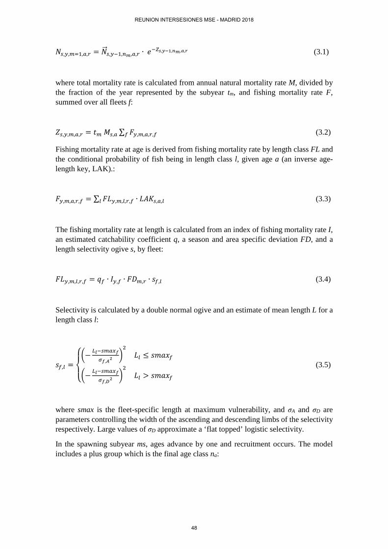
𝑁𝑁𝑠𝑠,𝑦𝑦,𝑚𝑚=1,𝑎𝑎,𝑟𝑟 = 𝑁𝑁��⃗ 𝑠𝑠,𝑦𝑦−1,𝑛𝑛𝑚𝑚,𝑎𝑎,𝑟𝑟 ∙ 𝑒𝑒−𝑍𝑍𝑠𝑠,𝑦𝑦−1,𝑛𝑛𝑚𝑚,𝑎𝑎,𝑟𝑟 (3.1)

where total mortality rate is calculated from annual natural mortality rate M, divided by the fraction of the year represented by the subyear tm, and fishing mortality rate F, summed over all fleets f:

𝑍𝑍𝑠𝑠,𝑦𝑦,𝑚𝑚,𝑎𝑎,𝑟𝑟 = 𝑡𝑡𝑚𝑚 𝑀𝑀𝑠𝑠,𝑎𝑎 ∑ 𝐹𝐹𝑦𝑦,𝑚𝑚,𝑎𝑎,𝑟𝑟,𝑓𝑓𝑓𝑓 (3.2)

Fishing mortality rate at age is derived from fishing mortality rate by length class FL and the conditional probability of fish being in length class l, given age a (an inverse age-length key, LAK).:

𝐹𝐹𝑦𝑦,𝑚𝑚,𝑎𝑎,𝑟𝑟,𝑓𝑓 = ∑ 𝐹𝐹𝐹𝐹𝑦𝑦,𝑚𝑚,𝑙𝑙,𝑟𝑟,𝑓𝑓𝑙𝑙 ∙ 𝐹𝐹𝐿𝐿𝐿𝐿𝑠𝑠,𝑎𝑎,𝑙𝑙 (3.3)

The fishing mortality rate at length is calculated from an index of fishing mortality rate I, an estimated catchability coefficient q, a season and area specific deviation FD, and a length selectivity ogive s, by fleet:

𝐹𝐹𝐹𝐹𝑦𝑦,𝑚𝑚,𝑙𝑙,𝑟𝑟,𝑓𝑓 = 𝑞𝑞𝑓𝑓 ∙ 𝐼𝐼𝑦𝑦,𝑓𝑓 ∙ 𝐹𝐹𝐹𝐹𝑚𝑚,𝑟𝑟 ∙ 𝑠𝑠𝑓𝑓,𝑙𝑙 (3.4)

Selectivity is calculated by a double normal ogive and an estimate of mean length L for a length class l:

𝑠𝑠𝑓𝑓,𝑙𝑙 =

⎩⎨

⎧�− 𝐿𝐿𝑙𝑙−𝑠𝑠𝑚𝑚𝑎𝑎𝑠𝑠𝑓𝑓𝜎𝜎𝑓𝑓,𝐴𝐴2

�2

𝐹𝐹𝑙𝑙 ≤ 𝑠𝑠𝑠𝑠𝑠𝑠𝑠𝑠𝑓𝑓

�− 𝐿𝐿𝑙𝑙−𝑠𝑠𝑚𝑚𝑎𝑎𝑠𝑠𝑓𝑓𝜎𝜎𝑓𝑓,𝐷𝐷2

�2

𝐹𝐹𝑙𝑙 > 𝑠𝑠𝑠𝑠𝑠𝑠𝑠𝑠𝑓𝑓 (3.5)

where smax is the fleet-specific length at maximum vulnerability, and σA and σD are parameters controlling the width of the ascending and descending limbs of the selectivity respectively. Large values of σD approximate a ‘flat topped’ logistic selectivity.

In the spawning subyear ms, ages advance by one and recruitment occurs. The model includes a plus group which is the final age class na:


48

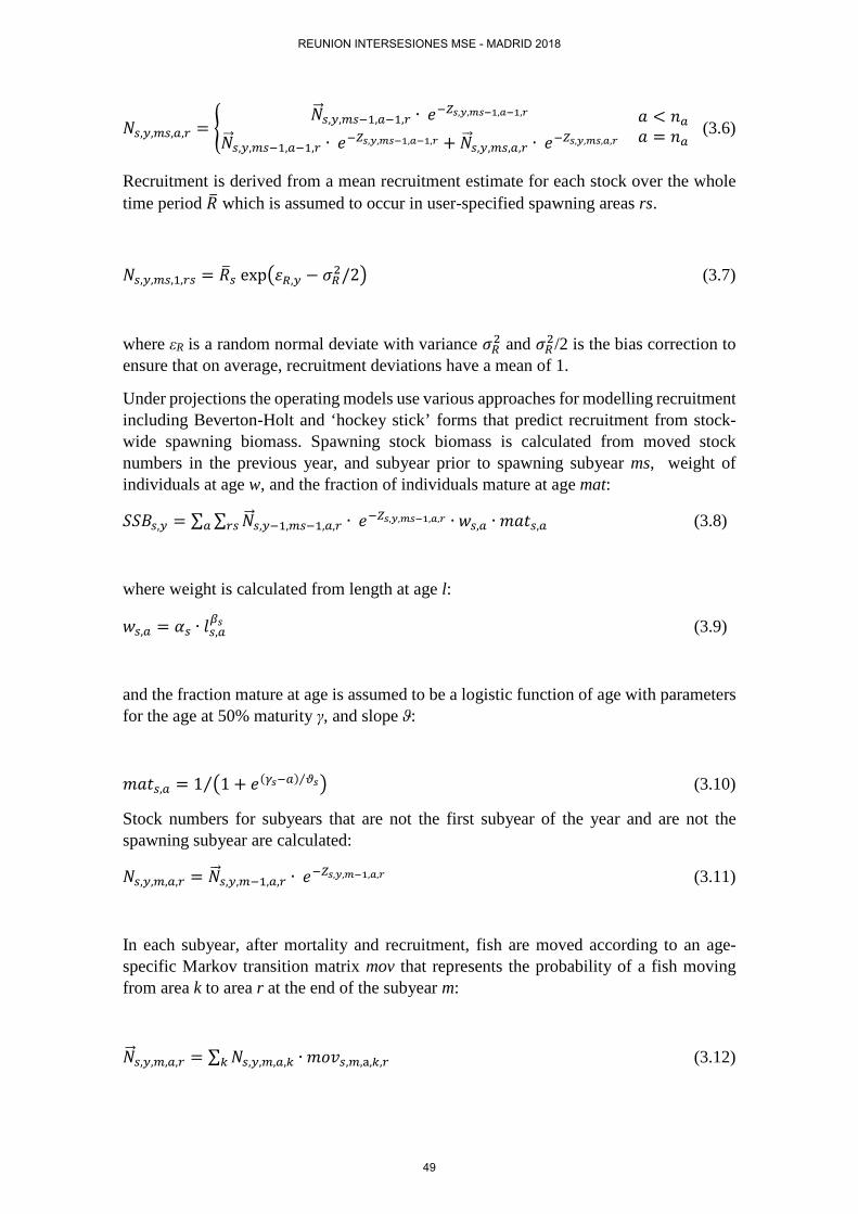
𝑁𝑁𝑠𝑠,𝑦𝑦,𝑚𝑚𝑠𝑠,𝑎𝑎,𝑟𝑟 = �𝑁𝑁��⃗ 𝑠𝑠,𝑦𝑦,𝑚𝑚𝑠𝑠−1,𝑎𝑎−1,𝑟𝑟 ∙ 𝑒𝑒−𝑍𝑍𝑠𝑠,𝑦𝑦,𝑚𝑚𝑠𝑠−1,𝑎𝑎−1,𝑟𝑟

𝑁𝑁��⃗ 𝑠𝑠,𝑦𝑦,𝑚𝑚𝑠𝑠−1,𝑎𝑎−1,𝑟𝑟 ∙ 𝑒𝑒−𝑍𝑍𝑠𝑠,𝑦𝑦,𝑚𝑚𝑠𝑠−1,𝑎𝑎−1,𝑟𝑟 + 𝑁𝑁��⃗ 𝑠𝑠,𝑦𝑦,𝑚𝑚𝑠𝑠,𝑎𝑎,𝑟𝑟 ∙ 𝑒𝑒−𝑍𝑍𝑠𝑠,𝑦𝑦,𝑚𝑚𝑠𝑠,𝑎𝑎,𝑟𝑟 𝑠𝑠 < 𝑛𝑛𝑎𝑎𝑠𝑠 = 𝑛𝑛𝑎𝑎

(3.6)

Recruitment is derived from a mean recruitment estimate for each stock over the whole time period 𝑅𝑅� which is assumed to occur in user-specified spawning areas rs.

𝑁𝑁𝑠𝑠,𝑦𝑦,𝑚𝑚𝑠𝑠,1,𝑟𝑟𝑠𝑠 = 𝑅𝑅�𝑠𝑠 exp �𝜀𝜀𝑅𝑅,𝑦𝑦 − 𝜎𝜎𝑅𝑅2/2� (3.7)

where εR is a random normal deviate with variance 𝜎𝜎𝑅𝑅2 and 𝜎𝜎𝑅𝑅2/2 is the bias correction to ensure that on average, recruitment deviations have a mean of 1.

Under projections the operating models use various approaches for modelling recruitment including Beverton-Holt and ‘hockey stick’ forms that predict recruitment from stock-wide spawning biomass. Spawning stock biomass is calculated from moved stock numbers in the previous year, and subyear prior to spawning subyear ms, weight of individuals at age w, and the fraction of individuals mature at age mat:

𝑆𝑆𝑆𝑆𝑆𝑆𝑠𝑠,𝑦𝑦 = ∑ ∑ 𝑁𝑁��⃗ 𝑠𝑠,𝑦𝑦−1,𝑚𝑚𝑠𝑠−1,𝑎𝑎,𝑟𝑟 ∙ 𝑒𝑒−𝑍𝑍𝑠𝑠,𝑦𝑦,𝑚𝑚𝑠𝑠−1,𝑎𝑎,𝑟𝑟𝑟𝑟𝑠𝑠𝑎𝑎 ∙ 𝑤𝑤𝑠𝑠,𝑎𝑎 ∙ 𝑠𝑠𝑠𝑠𝑡𝑡𝑠𝑠,𝑎𝑎 (3.8)

where weight is calculated from length at age l:

𝑤𝑤𝑠𝑠,𝑎𝑎 = 𝛼𝛼𝑠𝑠 ∙ 𝑙𝑙𝑠𝑠,𝑎𝑎𝛽𝛽𝑠𝑠 (3.9)

and the fraction mature at age is assumed to be a logistic function of age with parameters for the age at 50% maturity γ, and slope ϑ:

𝑠𝑠𝑠𝑠𝑡𝑡𝑠𝑠,𝑎𝑎 = 1 �1 + 𝑒𝑒(𝛾𝛾𝑠𝑠−𝑎𝑎) 𝜗𝜗𝑠𝑠⁄ �⁄ (3.10)

Stock numbers for subyears that are not the first subyear of the year and are not the spawning subyear are calculated:

𝑁𝑁𝑠𝑠,𝑦𝑦,𝑚𝑚,𝑎𝑎,𝑟𝑟 = 𝑁𝑁��⃗ 𝑠𝑠,𝑦𝑦,𝑚𝑚−1,𝑎𝑎,𝑟𝑟 ∙ 𝑒𝑒−𝑍𝑍𝑠𝑠,𝑦𝑦,𝑚𝑚−1,𝑎𝑎,𝑟𝑟 (3.11)

In each subyear, after mortality and recruitment, fish are moved according to an age-specific Markov transition matrix mov that represents the probability of a fish moving from area k to area r at the end of the subyear m:

𝑁𝑁��⃗ 𝑠𝑠,𝑦𝑦,𝑚𝑚,𝑎𝑎,𝑟𝑟 = ∑ 𝑁𝑁𝑠𝑠,𝑦𝑦,𝑚𝑚,𝑎𝑎,𝑘𝑘 ∙ 𝑠𝑠𝑚𝑚𝑚𝑚𝑠𝑠,𝑚𝑚,a,𝑘𝑘,𝑟𝑟𝑘𝑘 (3.12)


49

The movement matrix is calculated from a log-space matrix lnmov and a logit model to ensure each row (k) sums to 1:

𝑠𝑠𝑚𝑚𝑚𝑚𝑠𝑠,𝑚𝑚,a,𝑘𝑘,𝑟𝑟 = 𝑒𝑒𝑙𝑙𝑛𝑛𝑚𝑚𝑙𝑙𝑙𝑙𝑠𝑠,𝑚𝑚,a,𝑘𝑘,𝑟𝑟 ∑ 𝑒𝑒𝑙𝑙𝑛𝑛𝑚𝑚𝑙𝑙𝑙𝑙𝑠𝑠,𝑚𝑚,a,𝑘𝑘,𝑟𝑟𝑟𝑟⁄ (3.13)

Size/age stratification for movement models will initially be attempted for three age groups: 0-2, 3-8 and 9+ years (this will be kept the same for the Western Atlantic and the Eastern Atlantic/Mediterranean, but should be re-evaluated for the East as future data become available).

Movements from an area k to an area r that are considered to be implausible (e.g. from the Eastern Mediterranean to the Gulf of Mexico) are assigned a large negative number (essentially zero movement) in corresponding cells in these movement matrices. For each area k, from which individuals can move, one value is assigned zero and all other possible movements are assigned an estimated parameter ψ (since rows must sum to 1, there is one less degree of freedom):

𝑙𝑙𝑛𝑛𝑠𝑠𝑚𝑚𝑚𝑚𝑠𝑠,𝑚𝑚,𝑎𝑎,𝑘𝑘,𝑟𝑟 = �−1𝐶𝐶10

0𝛹𝛹𝑠𝑠,𝑚𝑚,𝑘𝑘,𝑟𝑟

𝑛𝑛𝑚𝑚 𝑠𝑠𝑚𝑚𝑚𝑚𝑒𝑒𝑠𝑠𝑒𝑒𝑛𝑛𝑡𝑡 𝑓𝑓𝑓𝑓𝑚𝑚𝑠𝑠 𝑘𝑘 𝑡𝑡𝑚𝑚 𝑓𝑓

𝑓𝑓𝑓𝑓𝑓𝑓𝑠𝑠𝑡𝑡 𝑠𝑠𝑠𝑠𝑠𝑠𝑓𝑓𝑎𝑎𝑛𝑛𝑒𝑒𝑎𝑎 𝑝𝑝𝑚𝑚𝑠𝑠𝑠𝑠𝑓𝑓𝑝𝑝𝑙𝑙𝑒𝑒 𝑠𝑠𝑚𝑚𝑚𝑚𝑒𝑒𝑠𝑠𝑒𝑒𝑛𝑛𝑡𝑡 𝑓𝑓𝑓𝑓𝑚𝑚𝑠𝑠 𝑘𝑘 𝑡𝑡𝑚𝑚 𝑓𝑓𝑚𝑚𝑡𝑡ℎ𝑒𝑒𝑓𝑓 𝑝𝑝𝑚𝑚𝑠𝑠𝑠𝑠𝑓𝑓𝑝𝑝𝑙𝑙𝑒𝑒 𝑠𝑠𝑚𝑚𝑚𝑚𝑒𝑒𝑠𝑠𝑒𝑒𝑛𝑛𝑡𝑡𝑠𝑠 𝑓𝑓𝑓𝑓𝑚𝑚𝑠𝑠 𝑘𝑘 𝑡𝑡𝑚𝑚 𝑓𝑓

(3.14)

This movement model can be simplified to estimate only those movements for which data have been observed (e.g.at least one tag track or conventional tagging observation).

Compared with spatially aggregated models, initialization is more complex for spatial models, particularly those that need to accommodate seasonal movement by age and may include regional spawning and recruitment. The equilibrium unfished age structure / spatial distribution cannot be calculated analytically. For any set of model parameters it is necessary to determine these numerically by iteratively multiplying an initial guess of age structure and spatial distribution by the movement matrix. The solution used here is to iterate the transition equations above (Equations 3.1, 3.6, 3.7, 3.11, 3.12) given a fishing mortality rate averaged over the first five years of model predictions until the spatial distribution of stock numbers converges for each of the subyears.

Prior to this iterative process an initial guess at the spatial and age structure of stock numbers 𝑁𝑁� is made based on the movement matrix and natural mortality rate at age M:

𝑁𝑁�𝑠𝑠,𝑚𝑚,𝑎𝑎,𝑟𝑟 = 𝑅𝑅�𝑠𝑠 ∙ e−∑ 𝑀𝑀𝑠𝑠,𝑎𝑎𝑎𝑎1 ∙ ∑ 1

𝑛𝑛𝑟𝑟∙ 𝑠𝑠𝑚𝑚𝑚𝑚𝑠𝑠,𝑚𝑚,a,𝑘𝑘,𝑟𝑟𝑘𝑘 (3.15)


50

In years prior to the initial model year (e.g. before 1983), historical catches 𝐶𝐶̅ for eastern and western areas (east/west of 45 degrees longitude) are used to initialize the model using stock reduction analysis (i.e. catches are removed without error from the asymptotic estimates of unfished numbers 𝑁𝑁�). Mean historical annual catches were divided up among areas and seasons assuming the same seasonal and spatial pattern of catches as the initial years of the modelled time series (e.g. 1961-1965).

Stock numbers for initialization years (e.g. 1864-1982) are calculated using the same equations (i.e. Eqn 3.11 and 3.12) as model years (e.g. 1983 – 2016). The exception is that rather than using effort data, selectivities and an inverse age-length key (Eqns 3.3 and 3.4), fishing mortality rate at age is derived from mean historical catches and the assumption is made that these are taken without error in the middle of the time step with natural mortality rate occurring both before and after fishing:

𝐹𝐹𝑖𝑖=1,𝑚𝑚,𝑎𝑎,𝑟𝑟,𝑓𝑓 =

⎩⎪⎨

⎪⎧ −log �1 − 𝐶𝐶�̅�𝑚,𝑎𝑎,𝑟𝑟

𝑁𝑁�𝑠𝑠,𝑚𝑚,𝑎𝑎,𝑟𝑟𝑒𝑒−�𝑡𝑡𝑚𝑚 𝑀𝑀𝑠𝑠,𝑎𝑎�/2� 𝑓𝑓 = 1

−log �1 − 𝐶𝐶�̅�𝑚,𝑎𝑎,𝑟𝑟

𝑁𝑁��⃗ 𝑠𝑠,𝑦𝑦−1,𝑛𝑛𝑚𝑚,𝑎𝑎,𝑟𝑟 𝑒𝑒−�𝑡𝑡𝑚𝑚 𝑀𝑀𝑠𝑠,𝑎𝑎�/2� 𝑓𝑓 > 1,𝑠𝑠 = 1

−log �1 − 𝐶𝐶�̅�𝑚,𝑎𝑎,𝑟𝑟

𝑁𝑁��⃗ 𝑠𝑠,𝑦𝑦,𝑚𝑚−1,𝑎𝑎,𝑟𝑟𝑒𝑒−�𝑡𝑡𝑚𝑚 𝑀𝑀𝑠𝑠,𝑎𝑎�/2� 𝑓𝑓 > 1,𝑠𝑠 > 1

(3.16)

where i=1 is the first year and calculates fishing mortality rates from asymptotic numbers 𝑁𝑁� (Eqn. 3.15).

Baseline Recruitment freely estimated (no stock-recruitment model assumed when fitting operating model to data)

Recruitment calculated from stock-wide SSB for projections only

Gravity movement model used to calculate Markov movement matrix by subyear and stock

Movement calculated only for those transitions recorded by tagging

Alternative options Hockey stick SR relationship (West) Recruitment calculated from spawning area SSB

Markov movement matrix by subyear and stock (following model updates the gravity model – a specific case of the more general Markov model – seemed an appropriate choice for the Baseline).

Movement calculated for all transitions except stock exclusive spawning areas.


51

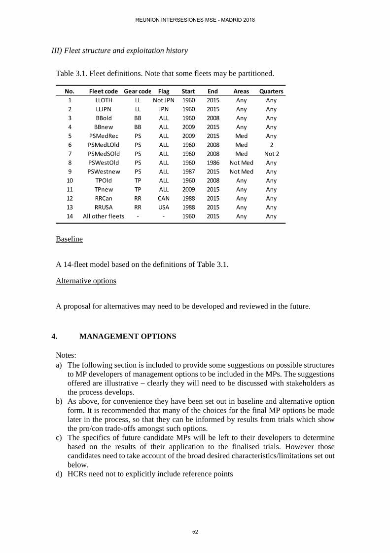
III) Fleet structure and exploitation history

Table 3.1. Fleet definitions. Note that some fleets may be partitioned.

Baseline

A 14-fleet model based on the definitions of Table 3.1.

Alternative options

A proposal for alternatives may need to be developed and reviewed in the future.

4. MANAGEMENT OPTIONS Notes: a) The following section is included to provide some suggestions on possible structures

to MP developers of management options to be included in the MPs. The suggestions offered are illustrative – clearly they will need to be discussed with stakeholders as the process develops.

b) As above, for convenience they have been set out in baseline and alternative option form. It is recommended that many of the choices for the final MP options be made later in the process, so that they can be informed by results from trials which show the pro/con trade-offs amongst such options.

c) The specifics of future candidate MPs will be left to their developers to determine based on the results of their application to the finalised trials. However those candidates need to take account of the broad desired characteristics/limitations set out below.

d) HCRs need not to explicitly include reference points

No. Fleet code Gear code Flag Start End Areas Quarters1 LLOTH LL Not JPN 1960 2015 Any Any2 LLJPN LL JPN 1960 2015 Any Any3 BBold BB ALL 1960 2008 Any Any4 BBnew BB ALL 2009 2015 Any Any5 PSMedRec PS ALL 2009 2015 Med Any6 PSMedLOld PS ALL 1960 2008 Med 27 PSMedSOld PS ALL 1960 2008 Med Not 28 PSWestOld PS ALL 1960 1986 Not Med Any9 PSWestnew PS ALL 1987 2015 Not Med Any

10 TPOld TP ALL 1960 2008 Any Any11 TPnew TP ALL 2009 2015 Any Any12 RRCan RR CAN 1988 2015 Any Any13 RRUSA RR USA 1988 2015 Any Any14 All other fleets - - 1960 2015 Any Any


52

I) Spatial strata for which TACs are set

Baseline

Conventional West and East/Mediterranean regions (Figure 1.1):

West: areas 1-4 (GOM, CAR, WATL, GSL).

East+Med: areas 5-10 (SCATL, NCATL, NEATL, EATL, SEATL, MED).

Alternative options

Various possibilities exist, based on alternative combinations of the spatial strata defined in Item 1. For example, separating out the central Atlantic (Figure 1.1A).

West: areas 1-4 (GOM, CAR, WATL, GSL).

Central: areas 5-6 (SCATL, NCATL).

East+Med: areas 7-10 (NEATL, EATL, SEATL, MED).

However it is suggested that consideration of such more complex options be postponed to a “second round”.

II) Options for the frequency of setting TACs

Baseline

Every two years, for both West and East+Med (or alternative spatial strata) together

Alternative options

i) Every three years ii) Every four years

III) Upper limits on TACs

[Note that this option has potential advantages for reducing risk and avoiding over-capitalisation.] Baseline No upper limit Alternative options West e.g. 5 000, 6 000 mt East +Med e.g. 30 000, 40 000 mt


53

IV) Minimum extent of TAC change

Baseline No minimum.

Alternative options West e.g. 200, 300 mt East +Med e.g. 1 000, 2 000 mt

V) Maximum extent of TAC change

[Note the underlying rationale is to promote industrial stability.]

Baseline West 20% East +Med 20%

Alternative options West 15% East +Med 15% Note that developers of candidate MPs should consider including options which: a) Override such restrictions on the maximum extent of reduction if abundance indices

drop below specified thresholds. b) Allow for greater increases (in terms of tonnage) if a TAC has had to be reduced to a

low level and indices confirm subsequent recovery.

VI) Technical measures Size restrictions might be considered on a fleet and/or spatial stratum basis. However, for a “first round” it is suggested that these not be included explicitly, but instead be considered to be effected implicitly through the selectivity prescriptions for future catches by the various fleets which are set out under item 6 below.

5. FUTURE RECRUITMENT AND DISTRIBUTION SCENARIOS See also section 9 of this document.


54

I) West

Functional forms fitted to assessment outputs for the years 1970+

a) Hockey stick b) Beverton Holt with steepness h estimated

II) East + Mediterranean

Functional forms fitted to years 1950+

a) Beverton Holt with h = 0.98 for 1950-1982, 1983+ and 1950+ b) Beverton Holt with h = 0.70 for 1950-1982, 1983+ and 1950+

Note that 1950-1982 is “low” recruitment, and 1983+ is “high” recruitment.

III) Future regime shifts

West a) None b) After 10 years of projection, switch to other regime c) Probability of 0.05 every projection year of switch to other regime

East+Med a) 1983+ relationship continues unchanged b) 1983+ relationship changes to 1950-1982 relationship after 10 years c) Probability of 0.05 every projection year of a swop between 1983+ and 1950-1982

relationships

Note that for option c), it might be better to preclude changes over, say, the last 10 years of a 30-year projection period to ease interpretation of results through the reduction of transient effects.

IV) Statistical properties

Residuals are taken to be lognormally distributed about the relationship assumed with the standard deviation of the log recruitments (σR) invariant over time.

Baseline

Uncorrelated residuals with σR = 0.5. (a common value obtained from the RAM legacy database).


55

Alternative options

σR and autocorrelation as estimated from the residuals for the conditioning concerned (post model fit, not within model fit, for greater statistical stability). For East+Med this will refer to the 1950+ fits.

V) Possible future distributional changes

Plausible options for future distributional changes (in relative terms) in response to changes in abundance and to possible environmental changes will be considered in a “second round”.

6. FUTURE CATCHES

Baseline a) Future catches will be taken to equal future TACs (up to a maximum harvest rate of

95%). b) The allocation of these future catches amongst fleets will be set equal to the average

over 2012-2014 c) The spatial distribution per stratum (see item 1 above) of these future catches will be

set equal to the average over 2012-2014 d) The selectivity function for each fleet for the most recent period for which this is

estimated in the conditioning of the trial concerned will be taken to apply for all future years

e) If the TAC is changed, the proportional allocation by fleet will remain unchanged, as will the proportional distribution by spatial stratum.

Alternative options

Clearly many are possible, but are probably best delayed until a “second round”. Were substantial changes to eventuate during a period when an MP was in operation, this would in any case likely necessitate re-tuning and re-testing or a modified MP.

The impacts of possible IUU catches should perhaps be considered under robustness trials (see item 9 below).

7. GENERATION OF FUTURE DATA Note that these are for use as input to MPs, so need to be chosen carefully from a set of those highly likely to be regularly (i.e. annually) available. This is because application of the MP relies on these data being available in this way, so difficulties can (and have in other cases) obviously arise should they fail to do so. Though any candidate MP proposed


56

should include a rule to deal with the absence of just one future value from an input series, any more than that would require re-tuning and re-testing of a modified MP, which is preferably planned to be avoided given the associated extra costs. Consideration is also needed of the “delays” associated in such data becoming available for input to an MP. The customary default is that for computation of the TAC for year y, the most recent data finalised and available will be for year y-2. Any changes to that will require motivation and specification.

I) Baseline suggestions

West a) Gulf of Mexico larval index of spawning stock abundance b) US RR 115-144cm index of exploitable abundance c) JLL_W CPUE index of exploitable abundance

East+Med a) JLL_NEA CPUE index of exploitable abundance b) Western Mediterranean larval index of spawning stock abundance c) GBYP aerial survey of adults d) Juvenile aerial survey Gulf of Lyon

II) Alternative options

Obviously many additions or alternatives to the suggestions made are possible. The reasons behind the initial suggestions above are respectively lengthy continuity (though admitting a concern about the decrease in spatial coverage of the JLL_NEA index over time) and fishery-independence. Accordingly the East + Med might be extended to include trap or baitboat indices.

Including additional indices of abundance will increase the workload (see below), so might be better postponed to a “second round”.

Catch-at-length series could also be considered for inclusion, but raise further technical complications regarding the specification of how they are generated, so are likely best deferred from consideration until a “second round”.

III) Relationships with abundance

For baseline trials, abundance indices will be taken to be linearly proportional to the appropriate component of the underlying model biomass in the stratum/strata concerned.

Possible alternatives to this are considered under Robustness trials (see item 9 below).


57

IV) Statistical properties

Baseline

a) Residuals are taken to be lognormally distributed; standard deviation of the log recruitments (σ) invariant over time.

b) The values of σ will be estimated c) No Autocorrelation of residuals d) The conditioning results will be inspected for model mis-specification regarding the

fit to the series concerned; if so the bias identified will be modelled to continue into the future in a “plausible” way.

Alternative options a) Fix σ values for all trials based on a central trial from the Reference set (see item 9

below). b) If additional CPUE indices to the single one initially suggested are included, residuals

need to be examined for correlation, with this being taken into account in generating future values.

Other aspects

Currently a ‘master’ relative abundance index is used for the Mixed stock model which provides an estimate of relative abundance across all time-area strata (e.g. by year, quarter and area). The approach taken here is to include multiple fleets by dividing their catches by this ‘master’ index to provide an index of fishing mortality rate (a partial F) leaving only catchability by fleet to be estimated rather than several thousands of individual F parameters (by fleet, year, quarter and area). Simulation testing reveals that this approach provides unbiased estimates of central quantities such as abundance, stock depletion, mixing rate and selectivity. However the construction of the ‘master’ index is critical and this is an important axis of uncertainty for operating models.

MP input series (e.g. as suggested in section I, above) may however be specific fleet indices, rather than this master relative abundance index, and hence require generation into the future. This will be effected by including these series in the conditioning with comparisons to the resource components which they are assumed to reflect, but with a very low weight in the log-likelihood so as not to impact estimates of other parameters in the model fit. The estimates of the catchability coefficients, and statistical properties of the residuals of this fit will be used in generating values for this series forward in time.

Note that consideration should at some stage also be given to new data types that are only now becoming available (e.g. aerial surveys, genetic tagging). These will not at this stage have been collected over a sufficient length of time to be able to serve as MP inputs, but the overall testing process can be used to provide insight into their potential future utility.


58

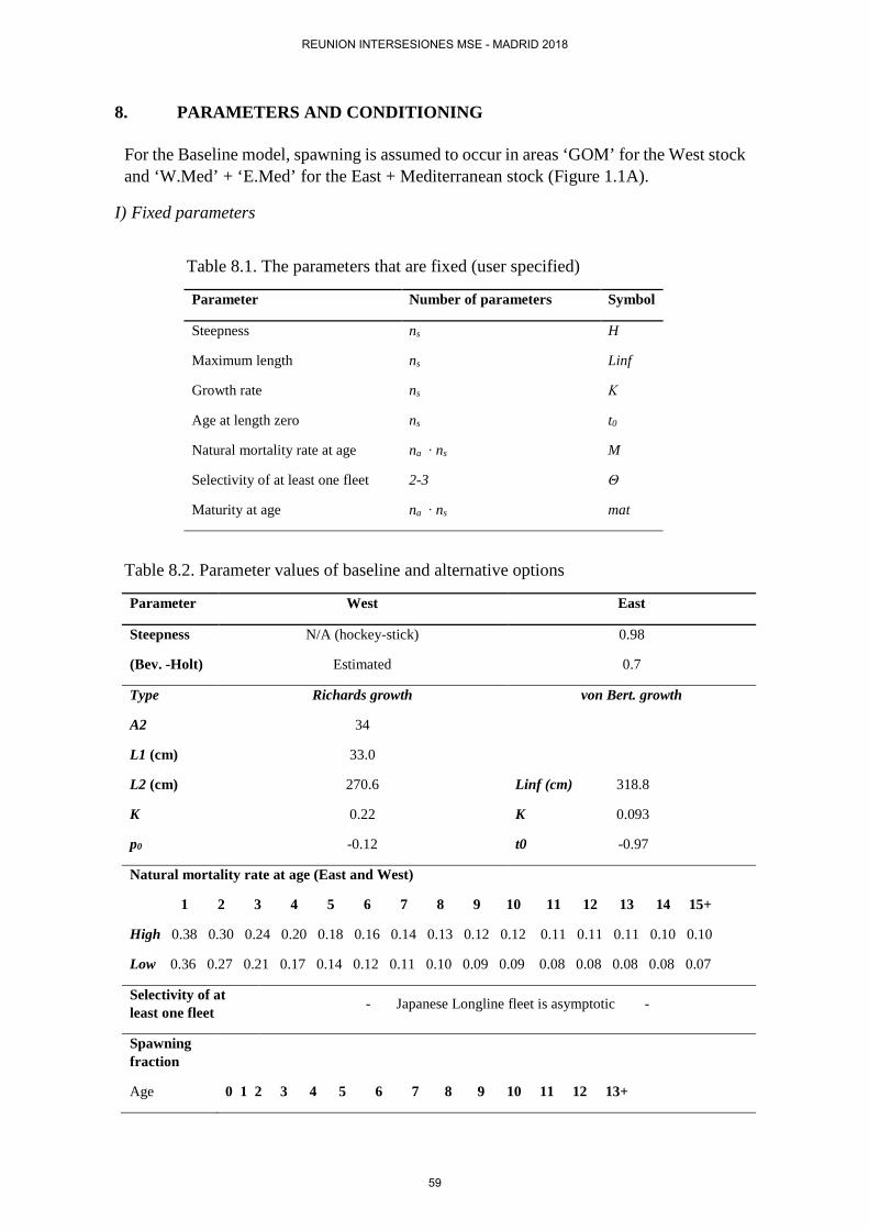
8. PARAMETERS AND CONDITIONING For the Baseline model, spawning is assumed to occur in areas ‘GOM’ for the West stock and ‘W.Med’ + ‘E.Med’ for the East + Mediterranean stock (Figure 1.1A).

I) Fixed parameters

Table 8.1. The parameters that are fixed (user specified)

Parameter Number of parameters Symbol

Steepness ns H

Maximum length ns Linf

Growth rate ns Κ

Age at length zero ns t0

Natural mortality rate at age na ∙ ns M

Selectivity of at least one fleet 2-3 Θ

Maturity at age na ∙ ns mat

Table 8.2. Parameter values of baseline and alternative options

Parameter West East

Steepness

(Bev. -Holt)

N/A (hockey-stick)

Estimated

0.98

0.7

Type Richards growth von Bert. growth

A2 34

L1 (cm) 33.0

L2 (cm) 270.6 Linf (cm) 318.8

K 0.22 K 0.093

p0 -0.12 t0 -0.97

Natural mortality rate at age (East and West)

1 2 3 4 5 6 7 8 9 10 11 12 13 14 15+

High 0.38 0.30 0.24 0.20 0.18 0.16 0.14 0.13 0.12 0.12 0.11 0.11 0.11 0.10 0.10

Low 0.36 0.27 0.21 0.17 0.14 0.12 0.11 0.10 0.09 0.09 0.08 0.08 0.08 0.08 0.07

Selectivity of at least one fleet - Japanese Longline fleet is asymptotic -

Spawning fraction

Age 0 1 2 3 4 5 6 7 8 9 10 11 12 13+


59

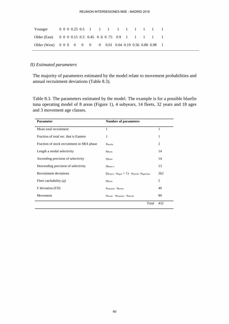
Younger

Older (East)

Older (West)

0 0 0 0.25 0.5 1 1 1 1 1 1 1 1 1

0 0 0 0.15 0.3 0.45 0 .6 0 .75 0.9 1 1 1 1 1

0 0 0 0 0 0 0 0.01 0.04 0.19 0.56 0.88 0.98 1

II) Estimated parameters The majority of parameters estimated by the model relate to movement probabilities and annual recruitment deviations (Table 8.3). Table 8.3. The parameters estimated by the model. The example is for a possible bluefin tuna operating model of 8 areas (Figure 1), 4 subyears, 14 fleets, 32 years and 18 ages and 3 movement age classes.

Parameter Number of parameters

Mean total recruitment 1 1

Fraction of total rec. that is Eastern 1 1

Fraction of stock recruitment in SRA phase nstocks 2

Length a modal selectivity nfleets 14

Ascending precision of selectivity nfleets 14

Descending precision of selectivity nfleets-1 13

Recruitment deviations (nyears + nages + 1) ∙ nstocks∙ nageclass 262

Fleet catchability (q) nfleets 5

F deviation (FD) nseasons ∙ nareas 40

Movement nareas ∙ nseasons ∙ nstocks 80

Total 432


60

Table 8.4. Prior probability distributions for model parameters with mean μ and standard deviation σ, and lower and upper bounds LB and UB, respectively.

Parameter Prior Likelihood component

All operating models

Total recruitment log-uniform(LB = 11.5, UB = 16.5) -lnLrec

Fraction of recruitment that is eastern

logit-uniform(LB = -∞, UB = ∞) -lnLfracrec

Fraction of stock recruitment in SRA phase

logit-uniform(LB = -2.0, UB = 2.0) -lnLhistrec

Selectivity lognormal(μ = 0, σ = 0.9) (LB = -3.0, UB = 3.0) -lnLsel

Fleet catchability (q) (mean F) log-uniform(LB = -10.0, UB = 1.0) -lnLq

Fishery independent index catchability

log-uniform(LB = -2.3, UB = 2.3) -lnLqI

Fishery dependent index catchability

log-uniform(LB = -6.0, UB = 4.0) -lnLqD

F deviation (FD, Eqn 3.4) lognormal(μ = 0, σ = 0.2) -lnLFD

Movement deviations (from fully mixed)

lognormal(μ = 0, σ = 1.0) (LB = -6.0, UB = 6.0) -lnLmov

Recruitment deviations lognormal(μ = 0, σ = 0.5) -lnLrecdev

Some operating models

Mean SSB by area (reference set, 2B)

lognormal(μEastern = ln(3E+5), μWestern =ln(2.7E+4), σ = 0.01) -lnLmuSSB

Eastern area SSB change (reference set, 2C)

lognormal(μ = ln(3), σ = 0.01) -lnLSSBinc

A summary of likelihood functions can be found in Table 8.4.

For each fleet f, total predicted catches in weight �̂�𝐶, are calculated from the Baranov equation:

�̂�𝐶𝑦𝑦,𝑚𝑚,𝑟𝑟,𝑓𝑓 = ∑ ∑ 𝑤𝑤𝑠𝑠,𝑎𝑎 ∙ 𝑁𝑁𝑠𝑠,𝑦𝑦,𝑚𝑚,𝑎𝑎,𝑟𝑟𝑎𝑎 ∙ (1 − 𝑒𝑒−𝑍𝑍𝑠𝑠,𝑦𝑦,𝑚𝑚,𝑎𝑎,𝑟𝑟) ∙ �𝐹𝐹𝑦𝑦,𝑚𝑚,𝑎𝑎,𝑟𝑟,𝑓𝑓

𝑍𝑍𝑠𝑠,𝑦𝑦,𝑚𝑚,𝑎𝑎,𝑟𝑟�𝑠𝑠 (8.1)

Similarly predicted catches in numbers at age (CAA) are given by:

𝐶𝐶𝐿𝐿𝐿𝐿�𝑠𝑠,𝑦𝑦,𝑚𝑚,𝑎𝑎,𝑟𝑟,𝑓𝑓 = 𝑁𝑁𝑠𝑠,𝑦𝑦,𝑚𝑚,𝑎𝑎,𝑟𝑟 ∙ (1 − 𝑒𝑒−𝑍𝑍𝑠𝑠,𝑦𝑦,𝑚𝑚,𝑎𝑎,𝑟𝑟) ∙ �𝐹𝐹𝑦𝑦,𝑚𝑚,𝑎𝑎,𝑟𝑟,𝑓𝑓

𝑍𝑍𝑠𝑠,𝑦𝑦,𝑚𝑚,𝑎𝑎,𝑟𝑟� (8.2)

This can be converted to a prediction of total catches in numbers by length class CAL using a stock specific inverse age-length key, LAK:


61

𝐶𝐶𝐿𝐿𝐹𝐹� 𝑦𝑦,𝑚𝑚,𝑙𝑙,𝑟𝑟,𝑓𝑓 = ∑ ∑ 𝐶𝐶𝐿𝐿𝐿𝐿�𝑠𝑠,𝑦𝑦,𝑚𝑚,𝑎𝑎,𝑟𝑟,𝑓𝑓 ∙ 𝐹𝐹𝐿𝐿𝐿𝐿𝑠𝑠,𝑎𝑎,𝑙𝑙𝑎𝑎𝑠𝑠 (8.3)

The model predicts spawning stock biomass indices 𝐼𝐼𝑠𝑠𝑠𝑠𝑝𝑝�, that are standardized to have a mean of 1 for each stock over the total number of years ny:

𝐼𝐼𝑠𝑠𝑠𝑠𝑝𝑝�𝑠𝑠,𝑦𝑦 = 𝑛𝑛𝑦𝑦 ∙ 𝑆𝑆𝑆𝑆𝑆𝑆𝑠𝑠,𝑦𝑦 ∑ 𝑆𝑆𝑆𝑆𝑆𝑆𝑠𝑠,𝑦𝑦𝑦𝑦⁄ (8.4)

The model predicts exploitable biomass indices 𝐼𝐼, by fleet that are standardized to have a mean of 1 for each fleet:

𝐼𝐼𝑦𝑦,𝑚𝑚,𝑟𝑟,𝑓𝑓 = 𝑛𝑛𝑦𝑦 ∙ 𝑛𝑛𝑚𝑚 ∙ 𝑛𝑛𝑟𝑟 ∙ 𝑉𝑉𝑦𝑦,𝑚𝑚,𝑟𝑟,𝑓𝑓 ∑ ∑ ∑ 𝑉𝑉𝑦𝑦,𝑚𝑚,𝑟𝑟,𝑓𝑓𝑟𝑟𝑚𝑚𝑦𝑦⁄ (8.5)

where exploitable biomass V is calculated as:

𝑉𝑉𝑦𝑦,𝑚𝑚,𝑟𝑟,𝑓𝑓 = ∑ �𝑠𝑠𝑓𝑓,𝑙𝑙 ∙ ∑ ∑ �𝑁𝑁𝑠𝑠,𝑦𝑦,𝑚𝑚,𝑎𝑎,𝑟𝑟,𝑓𝑓 ∙ 𝐹𝐹𝐿𝐿𝐿𝐿𝑠𝑠,𝑎𝑎,𝑙𝑙 ∙ 𝑤𝑤𝑠𝑠,𝑎𝑎�𝑎𝑎𝑠𝑠 �𝑙𝑙 (8.6)

The model predicts stock of origin composition of catches 𝑆𝑆𝑆𝑆𝑆𝑆�, from predicted catch numbers at age:

𝑆𝑆𝑆𝑆𝑆𝑆�𝑠𝑠,𝑦𝑦,𝑚𝑚,𝑟𝑟,𝑓𝑓 = ∑ 𝐶𝐶𝐿𝐿𝐿𝐿�𝑠𝑠,𝑦𝑦,𝑚𝑚,𝑎𝑎,𝑟𝑟,𝑓𝑓𝑎𝑎 ∑ ∑ 𝐶𝐶𝐿𝐿𝐿𝐿�𝑠𝑠,𝑦𝑦,𝑚𝑚,𝑎𝑎,𝑟𝑟,𝑓𝑓𝑎𝑎𝑠𝑠� (8.7)

A log-normal likelihood function is assumed for total catches by fleet. The negative log-likelihood is calculated as:

−𝑙𝑙𝑛𝑛𝐹𝐹𝑐𝑐 = ∑ ∑ ∑ ∑ 𝑙𝑙𝑛𝑛(𝜎𝜎𝑐𝑐𝑎𝑎𝑐𝑐𝑐𝑐ℎ) +�ln��̂�𝐶𝑦𝑦,𝑚𝑚,𝑟𝑟,𝑓𝑓�−ln�𝐶𝐶𝑦𝑦,𝑚𝑚,𝑟𝑟,𝑓𝑓��

2

2∙𝜎𝜎𝑐𝑐𝑎𝑎𝑡𝑡𝑐𝑐ℎ2𝑓𝑓𝑟𝑟𝑚𝑚𝑦𝑦 (8.8)

Similarly the negative log-likelihood components for indices of exploitable biomass and spawning stock biomass are calculated as:

−𝑙𝑙𝑛𝑛𝐹𝐹𝑖𝑖 = ∑ ∑ ∑ ∑ 𝑙𝑙𝑛𝑛(𝜎𝜎𝑖𝑖𝑛𝑛𝑖𝑖𝑒𝑒𝑠𝑠) +�𝑙𝑙𝑛𝑛�𝐼𝐼𝑦𝑦,𝑚𝑚,𝑟𝑟,𝑓𝑓�−𝑙𝑙𝑛𝑛�𝐼𝐼𝑦𝑦,𝑚𝑚,𝑟𝑟,𝑓𝑓��

2

2∙𝜎𝜎𝑖𝑖𝑛𝑛𝑖𝑖𝑖𝑖𝑖𝑖2𝑓𝑓𝑟𝑟𝑚𝑚𝑦𝑦 (8.9)


62

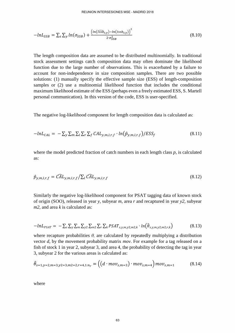
−𝑙𝑙𝑛𝑛𝐹𝐹𝑆𝑆𝑆𝑆𝑆𝑆 = ∑ ∑ 𝑙𝑙𝑛𝑛(𝜎𝜎𝑆𝑆𝑆𝑆𝑆𝑆) +�𝑙𝑙𝑛𝑛�𝐼𝐼𝑠𝑠𝑠𝑠𝐼𝐼�𝑠𝑠,𝑦𝑦�−𝑙𝑙𝑛𝑛�𝐼𝐼𝑠𝑠𝑠𝑠𝐼𝐼𝑠𝑠,𝑦𝑦��

2

2∙𝜎𝜎𝑆𝑆𝑆𝑆𝑆𝑆2𝑦𝑦𝑠𝑠 (8.10)

The length composition data are assumed to be distributed multinomially. In traditional stock assessment settings catch composition data may often dominate the likelihood function due to the large number of observations. This is exacerbated by a failure to account for non-independence in size composition samples. There are two possible solutions: (1) manually specify the effective sample size (ESS) of length-composition samples or (2) use a multinomial likelihood function that includes the conditional maximum likelihood estimate of the ESS (perhaps even a freely estimated ESS, S. Martell personal communication). In this version of the code, ESS is user-specified.

The negative log-likelihood component for length composition data is calculated as:

−𝑙𝑙𝑛𝑛𝐹𝐹𝐶𝐶𝐶𝐶𝐿𝐿 = −∑ ∑ ∑ ∑ ∑ 𝐶𝐶𝐿𝐿𝐹𝐹𝑦𝑦,𝑚𝑚,𝑙𝑙,𝑟𝑟,𝑓𝑓 ∙ 𝑙𝑙𝑛𝑛��̂�𝑝𝑦𝑦,𝑚𝑚,𝑙𝑙,𝑟𝑟,𝑓𝑓�/𝐶𝐶𝑆𝑆𝑆𝑆𝑓𝑓𝑓𝑓𝑟𝑟𝑙𝑙𝑚𝑚𝑦𝑦 (8.11)

where the model predicted fraction of catch numbers in each length class p, is calculated as:

�̂�𝑝𝑦𝑦,𝑚𝑚,𝑙𝑙,𝑟𝑟,𝑓𝑓 = 𝐶𝐶𝐿𝐿𝐹𝐹� 𝑦𝑦,𝑚𝑚,𝑙𝑙,𝑟𝑟,𝑓𝑓 ∑ 𝐶𝐶𝐿𝐿𝐹𝐹� 𝑦𝑦,𝑚𝑚,𝑙𝑙,𝑟𝑟,𝑓𝑓𝑙𝑙� (8.12)

Similarly the negative log-likelihood component for PSAT tagging data of known stock of origin (SOO), released in year y, subyear m, area r and recaptured in year y2, subyear m2, and area k is calculated as:

−𝑙𝑙𝑛𝑛𝐹𝐹𝐶𝐶𝑆𝑆𝐿𝐿𝑃𝑃 = −∑ ∑ ∑ ∑ ∑ ∑ ∑ 𝐶𝐶𝑆𝑆𝐿𝐿𝑃𝑃𝑠𝑠,𝑦𝑦,𝑠𝑠,𝑦𝑦2,𝑠𝑠2,𝑘𝑘 ∙ 𝑙𝑙𝑛𝑛�𝜃𝜃�𝑠𝑠,𝑦𝑦,𝑠𝑠,𝑦𝑦2,𝑠𝑠2,𝑓𝑓,𝑘𝑘�𝑘𝑘𝑓𝑓𝑠𝑠2𝑦𝑦2𝑠𝑠𝑦𝑦𝑠𝑠 (8.13)

where recapture probabilities θ, are calculated by repeatedly multiplying a distribution vector d, by the movement probability matrix mov. For example for a tag released on a fish of stock 1 in year 2, subyear 3, and area 4, the probability of detecting the tag in year 3, subyear 2 for the various areas is calculated as:

𝜃𝜃�𝑠𝑠=1,𝑦𝑦=2,𝑚𝑚=3,𝑦𝑦2=3,𝑚𝑚2=2,𝑟𝑟=4,1:𝑛𝑛𝑟𝑟 = ��𝑎𝑎 ∙ 𝑠𝑠𝑚𝑚𝑚𝑚𝑠𝑠,𝑚𝑚=3� ∙ 𝑠𝑠𝑚𝑚𝑚𝑚𝑠𝑠,𝑚𝑚=4�𝑠𝑠𝑚𝑚𝑚𝑚𝑠𝑠,𝑚𝑚=1 (8.14)

where


63

𝑎𝑎𝑘𝑘 = �01 𝑘𝑘 ≠ 𝑓𝑓𝑘𝑘 = 𝑓𝑓

(8.15)

The negative log-likelihood component for PSAT tagging data of unknown stock of origin PSATu, is currently weighted according to the compound probability that a fish is of a particular stock given the track history for that tag. For example for a tag t, tracked in series of years yi, subyears mi, and regions ri, the weight w, of that tag for a specific stock is calculated as:

𝑤𝑤𝑐𝑐,𝑠𝑠 =∏ ��∑ 𝑁𝑁𝑠𝑠𝑖𝑖,𝑦𝑦𝑖𝑖,𝑚𝑚𝑖𝑖,𝑎𝑎𝑖𝑖,𝑟𝑟𝑖𝑖𝑎𝑎 � �∑ ∑ 𝑁𝑁𝑠𝑠𝑖𝑖,𝑦𝑦𝑖𝑖,𝑚𝑚𝑖𝑖,𝑎𝑎𝑖𝑖,𝑟𝑟𝑖𝑖𝑎𝑎𝒔𝒔 �� 𝑖𝑖

∏ �1−�∑ 𝑁𝑁𝑠𝑠𝑖𝑖,𝑦𝑦𝑖𝑖,𝑚𝑚𝑖𝑖,𝑎𝑎𝑖𝑖,𝑟𝑟𝑖𝑖𝑎𝑎 � �∑ ∑ 𝑁𝑁𝑠𝑠𝑖𝑖,𝑦𝑦𝑖𝑖,𝑚𝑚𝑖𝑖,𝑎𝑎𝑖𝑖,𝑟𝑟𝑖𝑖𝑎𝑎𝒔𝒔 �� 𝑖𝑖 (8.16)

This is simply the product of fractions of that stock in those time-area strata divided by the product of the fractions of other stocks in those time-area strata. An alternative approach would be to compare the relative probabilities of the observed movements among the stocks although it is unclear whether this circularity (PSAT data are a primary source of information regarding movement) could lead to estimation problems.

The weighted negative log-likelihood function is similar to that of the stocks of known origin but includes the appropriate weighting term for each tag:

−𝑙𝑙𝑛𝑛𝐹𝐹𝑃𝑃𝑆𝑆𝐶𝐶𝑃𝑃 = −� � � � � � � � 𝐶𝐶𝑆𝑆𝐿𝐿𝑃𝑃𝑃𝑃𝑐𝑐,𝑠𝑠,𝑦𝑦,𝑚𝑚,𝑦𝑦2,𝑚𝑚2,𝑘𝑘𝑘𝑘𝑟𝑟𝑚𝑚2𝑦𝑦2𝑚𝑚𝑦𝑦𝑠𝑠𝑐𝑐

∙ 𝑙𝑙𝑛𝑛�𝜃𝜃�𝑠𝑠,𝑦𝑦,𝑚𝑚,𝑦𝑦2,𝑚𝑚2,𝑟𝑟,𝑘𝑘� ∙ 𝑤𝑤𝑐𝑐,𝑠𝑠 (8.17)

The negative log-likelihood component for stock of origin data SOO is also calculated assuming a multinomial distribution:

−𝑙𝑙𝑛𝑛𝐹𝐹𝑆𝑆𝑆𝑆𝑆𝑆 = −∑ ∑ ∑ ∑ ∑ 𝑆𝑆𝑆𝑆𝑆𝑆𝑠𝑠,𝑦𝑦,𝒎𝒎,𝒓𝒓,𝒇𝒇 ∙ 𝑙𝑙𝑛𝑛�𝑆𝑆𝑆𝑆𝑆𝑆�𝑠𝑠,𝑦𝑦,𝑚𝑚,𝑟𝑟,𝑓𝑓�𝒇𝒇𝑟𝑟𝑚𝑚𝑦𝑦𝒔𝒔 (8.18)

In order to fit the operating models to assessment model predictions (Factor 2 level B) a likelihood function is included for mean spawning 𝑆𝑆𝑆𝑆𝑆𝑆�� by Eastern/Western area k,


64

−𝑙𝑙𝑛𝑛𝐹𝐹𝑚𝑚𝑚𝑚𝑆𝑆𝑆𝑆𝑆𝑆 = ∑ 𝑙𝑙𝑛𝑛(𝜎𝜎𝑚𝑚𝑚𝑚𝑆𝑆𝑆𝑆𝑆𝑆) +�ln(𝑆𝑆𝑆𝑆𝑆𝑆��𝑘𝑘)−ln�𝑆𝑆𝑆𝑆𝑆𝑆��

𝑘𝑘��2

2∙𝜎𝜎𝑚𝑚𝑚𝑚𝑆𝑆𝑆𝑆𝑆𝑆2𝑘𝑘

(8.19)

where 𝑆𝑆𝑆𝑆𝑆𝑆�� is the mean annual SSB estimated from the VPA stock assessments (around 300 000 tonnes in the East, 27 000 tonnes in the West) and operating model predicted spawning biomass 𝑆𝑆𝑆𝑆𝑆𝑆�� is calculated:

𝑆𝑆𝑆𝑆𝑆𝑆��𝑘𝑘 = 1𝑛𝑛𝑦𝑦𝑛𝑛𝑚𝑚

∑ ∑ ∑ ∑ ∑ (𝑁𝑁��⃗ 𝑠𝑠,𝑦𝑦−1,𝑚𝑚𝑠𝑠−1,𝑎𝑎,𝑟𝑟 ∙ 𝑒𝑒−𝑍𝑍𝑠𝑠,𝑦𝑦,𝑚𝑚𝑠𝑠−1,𝑎𝑎,𝑟𝑟𝑟𝑟𝑎𝑎 ∙ 𝑤𝑤𝑠𝑠,𝑎𝑎 ∙ 𝑠𝑠𝑠𝑠𝑡𝑡𝑠𝑠,𝑎𝑎𝑚𝑚 )𝑠𝑠𝑦𝑦𝑎𝑎𝑟𝑟𝑒𝑒𝑎𝑎𝑘𝑘,𝑟𝑟

(8.20)

and area is a switch that is either 1 or zero depending on whether the area r is in the Eastern or Western assessment areas.

In order to fit the operating models to assessment model spawning biomass increases (Factor 2 level C) a likelihood function is included for spawning biomass increases by area:

−𝑙𝑙𝑛𝑛𝐹𝐹𝑆𝑆𝑆𝑆𝑆𝑆𝑖𝑖𝑛𝑛𝑐𝑐 = ∑ 𝑙𝑙𝑛𝑛(𝜎𝜎𝑆𝑆𝑆𝑆𝑆𝑆𝑖𝑖𝑛𝑛𝑐𝑐) +�ln�

𝑆𝑆𝑆𝑆𝑆𝑆𝑘𝑘,𝑦𝑦2𝑆𝑆𝑆𝑆𝑆𝑆𝑘𝑘,𝑦𝑦1

�−ln(𝑆𝑆𝑆𝑆𝑆𝑆𝑖𝑖𝑛𝑛𝑐𝑐)�2

2∙𝜎𝜎𝑆𝑆𝑆𝑆𝑆𝑆𝑖𝑖𝑛𝑛𝑐𝑐2𝑘𝑘

(8.21)

where SSB is the spawning biomass in eastern/western area k and SSBinc is the fractional increase in VPA assessment spawning biomass in area k from year y1 to year y2 (this is 3 between years 2006 and 2015).

The global penalised negative log-likelihood -lnLT, to be minimized is the summation of the weighted negative log-likelihood components for the data and priors (Table 8.4):

−𝑙𝑙𝑛𝑛𝐹𝐹𝑃𝑃 = −[𝜔𝜔𝑐𝑐 ∙ 𝑙𝑙𝑛𝑛𝐹𝐹𝑐𝑐 + 𝜔𝜔𝑖𝑖 ∙ 𝑙𝑙𝑛𝑛𝐹𝐹𝑖𝑖 + 𝜔𝜔𝑆𝑆𝑆𝑆𝑆𝑆 ∙ 𝑙𝑙𝑛𝑛𝐹𝐹𝑆𝑆𝑆𝑆𝑆𝑆 + 𝜔𝜔𝐶𝐶𝐶𝐶𝐿𝐿 ∙ 𝑙𝑙𝑛𝑛𝐹𝐹𝐶𝐶𝐶𝐶𝐿𝐿 +

𝜔𝜔𝑃𝑃𝑆𝑆𝐶𝐶𝑃𝑃 ∙ 𝑙𝑙𝑛𝑛𝐹𝐹𝑃𝑃𝑆𝑆𝐶𝐶𝑃𝑃 + 𝜔𝜔𝑆𝑆𝑆𝑆𝑆𝑆 ∙ 𝑙𝑙𝑛𝑛𝐹𝐹𝑆𝑆𝑆𝑆𝑆𝑆 + 𝜔𝜔𝑚𝑚𝑚𝑚𝑆𝑆𝑆𝑆𝑆𝑆 ∙ 𝑙𝑙𝑛𝑛𝐹𝐹𝑚𝑚𝑚𝑚𝑆𝑆𝑆𝑆𝑆𝑆 + 𝜔𝜔𝑆𝑆𝑆𝑆𝑆𝑆𝑖𝑖𝑛𝑛𝑐𝑐 ∙𝑙𝑙𝑛𝑛𝐹𝐹𝑆𝑆𝑆𝑆𝑆𝑆𝑖𝑖𝑛𝑛𝑐𝑐 + 𝜔𝜔𝑟𝑟𝑒𝑒𝑐𝑐 ∙ 𝑙𝑙𝑛𝑛𝐹𝐹𝑟𝑟𝑒𝑒𝑐𝑐 + 𝜔𝜔𝑓𝑓𝑟𝑟𝑎𝑎𝑐𝑐𝑟𝑟𝑒𝑒𝑐𝑐 ∙ 𝑙𝑙𝑛𝑛𝐹𝐹𝑓𝑓𝑟𝑟𝑎𝑎𝑐𝑐𝑟𝑟𝑒𝑒𝑐𝑐 + 𝜔𝜔ℎ𝑖𝑖𝑠𝑠𝑐𝑐𝑟𝑟𝑒𝑒𝑐𝑐 ∙𝑙𝑙𝑛𝑛𝐹𝐹ℎ𝑖𝑖𝑠𝑠𝑐𝑐𝑟𝑟𝑒𝑒𝑐𝑐 + 𝜔𝜔𝑠𝑠𝑒𝑒𝑙𝑙 ∙ 𝑙𝑙𝑛𝑛𝐹𝐹𝑠𝑠𝑒𝑒𝑙𝑙 + 𝜔𝜔𝑞𝑞 ∙ 𝑙𝑙𝑛𝑛𝐹𝐹𝑞𝑞 + 𝜔𝜔𝑞𝑞𝐼𝐼 ∙ 𝑙𝑙𝑛𝑛𝐹𝐹𝑞𝑞𝐼𝐼 + 𝜔𝜔𝑞𝑞𝑞𝑞 ∙ 𝑙𝑙𝑛𝑛𝐹𝐹𝑞𝑞𝑞𝑞 +𝜔𝜔𝐹𝐹𝑞𝑞 ∙ 𝑙𝑙𝑛𝑛𝐹𝐹𝐹𝐹𝑞𝑞 + 𝜔𝜔𝑚𝑚𝑙𝑙𝑙𝑙 ∙ 𝑙𝑙𝑛𝑛𝐹𝐹𝑚𝑚𝑙𝑙𝑙𝑙 + 𝜔𝜔𝑟𝑟𝑒𝑒𝑐𝑐𝑖𝑖𝑒𝑒𝑙𝑙 ∙ 𝑙𝑙𝑛𝑛𝐹𝐹𝑟𝑟𝑒𝑒𝑐𝑐𝑖𝑖𝑒𝑒𝑙𝑙] (8.22)


65

Table 8.5. Summary of the negative log-likelihood function contributions from various data

Type of data Disaggregation Function Likelihood component

Total catches (weight) year, subyear, area, fleet Log-normal lnLc

Index of exploitable biomass (assessment CPUE index) year, subyear, area, fleet Log-normal lnLi

Index of spawning stock biomass (e.g. a larval survey)

year, stock Log-normal lnLSSB

Length composition year, subyear, area Multinomial lnLCAL

PSAT tag (known stock of origin) stock, year, subyear, area, age class Multinomial lnLPSAT

Stock of origin year, subyear, area, age class Multinomial lnLSOO

III) Characterising uncertainty

Baseline

Include within-model uncertainty via MCMC sampling of posteriors for model parameters.

Alternative options

Include within-model uncertainty (parameter uncertainty) via Monte Carlo sampling from the inverse Hessian matrix of model parameters.

Concentrate on among-model uncertainty using the maximum posterior density estimates of model parameters and a prior model weight based on expert judgement. Uniform weights will be used to start, possibly updated later using a Delphi-type approach.


66

9. TRIAL SPECIFICATIONS

A. Reference set

Three major uncertainty axes: future recruitment; current abundance; and natural mortality/maturity (in combination) for conditioning and projections. These axes assume that the options of East and West are linked across rows of the table below. This is done with the intention of capturing extremes.

West East

Future recruitment

1 Hockey-stick 83+ B-H with h=0.98

2 B-H with h estimated 83+ B-H with h=0.70

3 Hockey-stick changes to

B-H after 10 years 83+ B-H with h=0.98 changes to 50-82 B-H with h=0.98 after 10 years

Abundance

A Best estimate

B East-West area spawning biomass matches VPA assessment

C Recent eastern area SSB increases 3x to match VPA assessment

Spawning fraction both stocks Natural Mortality rate both stocks

I Younger High

II Younger Low

III Older High

IV Older Low

Note: when modifying current abundance a highly informative prior will be placed on either the spawning biomass by Eastern-Western area (B) or the trend (fractional increase) in the eastern area (C).

Combinations for Reference Set

A full cross of (1, 2, 3) x (A, B, C) x (I, II, III, IV), i.e. 36 scenarios in total.

Discussion will be required regarding whether, in addition to considering results for each of these scenarios individually, they should also be considered for all scenarios in combination, and if so how the scenarios should be weighted (if at all) in such a combination.


67

B. Robustness trials

High priority

1) Future catches in both the West and the East+Med are each year 20% bigger than the TAC as a result of IUU fishing (of which the MP is not aware)

2) An undetected increase in catchability for CPUE-based abundance indices of 1% per annum

3) Non-linear index-abundance relationships 4) Alternative mixing scenario 5) Reference OM #1 assumptions but forcing SSB fit to that of the Western VPA

assessment Low priority

1) Future recruitment change as in 3), but with prob of 0.05 for each of the first 20 years of projection

2) Alternative assignments to stock of origin of historical catches from the South Atlantic (off Brazil)

“Second round” issues

The following aspects of uncertainty are suggested to be postponed at this time for consideration rather in a “second round”:

1) More than two stocks 2) More than two indices of abundance used as input to a MP 3) Use of CAL data in an MP 4) TACs allocated on a spatially more complex basis than the traditional west and

East+Med 5) Changes in technical measures affecting selectivity 6) Changes in stock distributions in the future 7) Future changes in proportional allocation of TACs amongst fleets

10. PERFORMANCE MEASURES/STATISTICS Projections under candidate MPs will be for 100 years (unless this leads to computational difficulties) commencing in 2017. Prior to that, for projecting for years between the last year of the condition and 2017, the catches will be set equal to the TACs already set, with abundance index data (and any further monitoring data such as catch-at-length) not yet available for those years being generated as specified under item 7. Note that considering a period as lengthy as 100 years is not to imply high reliability for projections for such a long time, but to be able take account of transient effects that persist for some time for a long-lived species.


68

I) Summary measures/statistics a) Annual average catch for the first, second and third 10-year period of MP application

(C10, C20 and C30, respectively). b) Spawning biomass depletion calculated relative to the deterministic equilibrium in the

absence of catches for the recruitment function that applies after 10, 20 and 30 years of MP application (D10, D20 and D30, respectively)

c) The lowest spawning biomass depletion over the 30 years for which the MP is applied (LD).

d) Spawning biomass depletion after 30 years, but calculated relative to the trajectory that would have occurred had no catches been taken over the full period for which MP application is being considered (DNC)

e) The lowest spawning biomass depletion over the 30 years for which the MP is applied, but calculated relative to the zero catch trajectory specified in d (LDNC).

f) Kobe or alternative Kobe indicators: catch/biomass instead of Fmsy (POF); and biomass/biomass at a theoretical maximum MSY (POS); and the probability of both underfishing and underfished status (probability green kobe zone: PGK).

g) Average annual variation in catches (AAVC) defined by:

∑=

−−−=2046

20171130

1y

yyy CCCAAV (13.1)

For each of these distributions, 5%-, 50%- and 95%iles are to be reported from 200 replicates. Note the reason for measures/statistics c) and e) is to compensate for regime changes. The choice of these percentiles may need further exploration with stakeholders.

Further stakeholder orientated measures may need to be included. These must be scientifically based, easily understood by stakeholders and such that managers may readily request the evaluation of any changes in options.

II) Summary plots Catch and spawning biomass trajectories plotted as:

a) Annual medians with 5%- and 95%-ile envelopes b) 10 worm plots of individual realisations

Note that repetitions for different options for selectivity may be needed.


69

III) Level of reporting

Baseline

a) Catch-related measures/statistics by traditional West and East+Med regions. b) Spawning biomass depletions measures/statistics by separate stocks

Alternative options

Many can be conceived, likely related primarily to catch and depletion by some combination of stock and/or spatial stratum. However these might be left for a “second round”, as they would become more pertinent in the face of greater model complexities possibly introduced at that time, such as changing spatial distributions of stocks and/or catches (resulting from changed proportional allocations to different fleets).


70

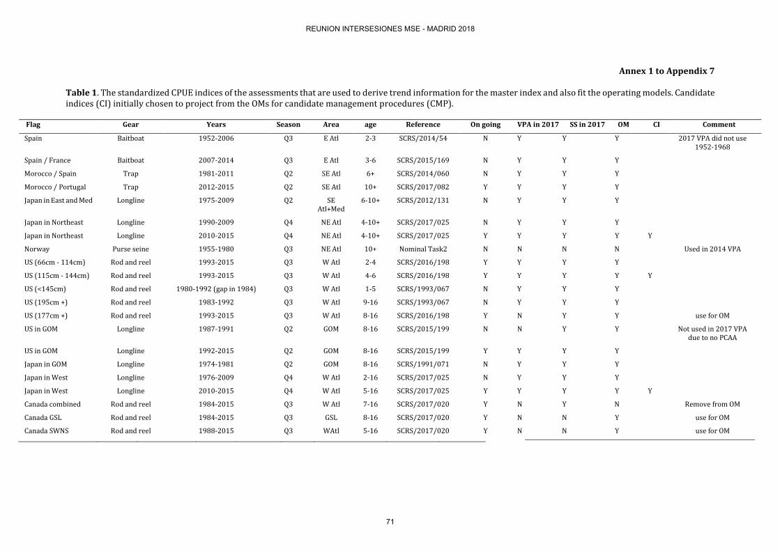
Annex 1 to Appendix 7

Table 1. The standardized CPUE indices of the assessments that are used to derive trend information for the master index and also fit the operating models. Candidate indices (CI) initially chosen to project from the OMs for candidate management procedures (CMP).

Flag Gear Years Season Area age Reference On going VPA in 2017 SS in 2017 OM CI Comment

Spain Baitboat 1952-2006 Q3 E Atl 2-3 SCRS/2014/54 N Y Y Y 2017 VPA did not use 1952-1968

Spain / France Baitboat 2007-2014 Q3 E Atl 3-6 SCRS/2015/169 N Y Y Y

Morocco / Spain Trap 1981-2011 Q2 SE Atl 6+ SCRS/2014/060 N Y Y Y

Morocco / Portugal Trap 2012-2015 Q2 SE Atl 10+ SCRS/2017/082 Y Y Y Y

Japan in East and Med Longline 1975-2009 Q2 SE Atl+Med

6-10+ SCRS/2012/131 N Y Y Y

Japan in Northeast Longline 1990-2009 Q4 NE Atl 4-10+ SCRS/2017/025 N Y Y Y

Japan in Northeast Longline 2010-2015 Q4 NE Atl 4-10+ SCRS/2017/025 Y Y Y Y Y

Norway Purse seine 1955-1980 Q3 NE Atl 10+ Nominal Task2 N N N N Used in 2014 VPA

US (66cm - 114cm) Rod and reel 1993-2015 Q3 W Atl 2-4 SCRS/2016/198 Y Y Y Y

US (115cm - 144cm) Rod and reel 1993-2015 Q3 W Atl 4-6 SCRS/2016/198 Y Y Y Y Y

US (<145cm) Rod and reel 1980-1992 (gap in 1984) Q3 W Atl 1-5 SCRS/1993/067 N Y Y Y

US (195cm +) Rod and reel 1983-1992 Q3 W Atl 9-16 SCRS/1993/067 N Y Y Y

US (177cm +) Rod and reel 1993-2015 Q3 W Atl 8-16 SCRS/2016/198 Y N Y Y use for OM

US in GOM Longline 1987-1991 Q2 GOM 8-16 SCRS/2015/199 N N Y Y Not used in 2017 VPA due to no PCAA

US in GOM Longline 1992-2015 Q2 GOM 8-16 SCRS/2015/199 Y Y Y Y

Japan in GOM Longline 1974-1981 Q2 GOM 8-16 SCRS/1991/071 N Y Y Y

Japan in West Longline 1976-2009 Q4 W Atl 2-16 SCRS/2017/025 N Y Y Y

Japan in West Longline 2010-2015 Q4 W Atl 5-16 SCRS/2017/025 Y Y Y Y Y

Canada combined Rod and reel 1984-2015 Q3 W Atl 7-16 SCRS/2017/020 Y N Y N Remove from OM

Canada GSL Rod and reel 1984-2015 Q3 GSL 8-16 SCRS/2017/020 Y N N Y use for OM

Canada SWNS Rod and reel 1988-2015 Q3 WAtl 5-16 SCRS/2017/020 Y N N Y use for OM


71

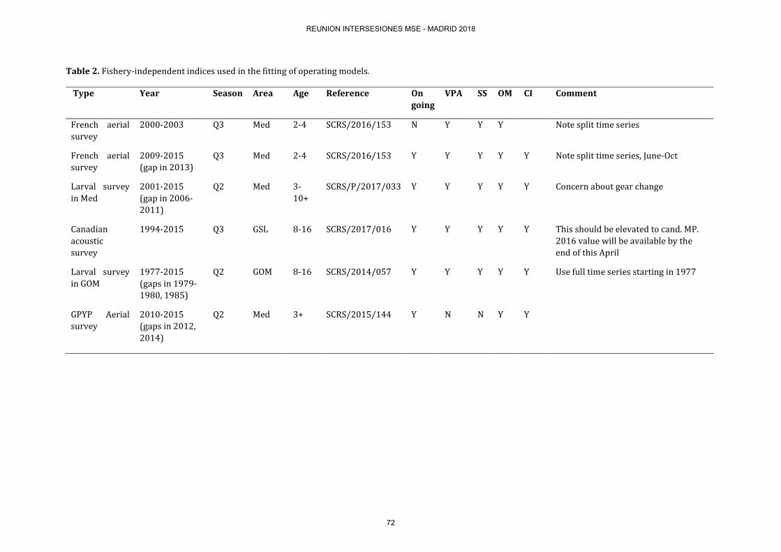
Table 2. Fishery-independent indices used in the fitting of operating models.

Type Year Season Area Age Reference On going

VPA SS OM CI Comment

French aerial survey

2000-2003 Q3 Med 2-4 SCRS/2016/153 N Y Y Y Note split time series

French aerial survey

2009-2015 (gap in 2013)

Q3 Med 2-4 SCRS/2016/153 Y Y Y Y Y Note split time series, June-Oct

Larval survey in Med

2001-2015 (gap in 2006-2011)

Q2 Med 3-10+

SCRS/P/2017/033 Y Y Y Y Y Concern about gear change

Canadian acoustic survey

1994-2015 Q3 GSL 8-16 SCRS/2017/016 Y Y Y Y Y This should be elevated to cand. MP. 2016 value will be available by the end of this April

Larval survey in GOM

1977-2015 (gaps in 1979-1980, 1985)

Q2 GOM 8-16 SCRS/2014/057 Y Y Y Y Y Use full time series starting in 1977

GPYP Aerial survey

2010-2015 (gaps in 2012, 2014)

Q2 Med 3+ SCRS/2015/144 Y N N Y Y


72

Appendix 8

TUNING OF CMPs (D. Butterworth)

Tuning (adjustment on CMP control parameter values) of CMPs conventionally takes place at two stages of the MSE process, and for two quite different reasons and audiences. CMP development At this stage there will be a number of CMP developers. Each will have their preferred CMP(s) (with their associated control parameter values/tunings) which have been adjusted for results somewhere on the axis from very conservative to highly aggressive as regards the catch vs resource depletion trade-off. This then causes a problem in comparing results from the preferred MPs provided by different developers who will have made different selections along this axis, because comparisons are confounded by these differences. The purpose of “development tuning” is to remove this confounding so as to compare on a level playing field. It is achieved by each developer, in addition to their own preferred tuning, providing results for a common alternative tuning which meets some specified performance criterion. This is typically expressed in terms of resource depletion for a particular OM. For example, this might be that median spawning biomass should equal SSB(MSY) after 30 years of projection for OM1. The reasons this is done is that such comparisons provide important insight into the properties of a CMP through such fair comparison with similar results for another. For example, performance across the other OMs might show that procedure to be less robust to uncertainty in its performance compared to another CMP. Further, in seeing where his/her CMP performs worse than another CMP, a developer learns where to concentrate in improving their CMP (for their preferred tuning). This development tuning and its results are considered only within the technical scientific sub-group involved in the MSE process. MP finalisation “Finalisation tuning” takes place only during the last stages of the MSE process, when one or a few CMPs are being selected for recommendation to the Commission. At that stage of the process:

- Only one or two CMPs will have survived. - The Commission will have provided feedback as to the range of catch vs depletion options it wishes

to consider. - The overview scientific committee (e.g. the bluefin session) will have agreed how results are to be

weighted over a Reference Set of OMs to provide aggregate performance statistics.

Thus for example, this feedback might have indicated an objective to be securing spawning biomass after 30 years to be close to SSB(MSY). The finalisation tuning would then adjust CMP control parameters to provide a median SSB after those 30 years for this statistic weighted over the Reference Set OMs as agreed. If options are requested by the Commission, then three finalisation tunings of each surviving CMP to be reported might correspond to: Median (SSB(30)/SSB(MSY)) = 0.9; 1.0; and 1.1 Current proposal The current proposal concerns ONLY “development tuning” (decisions regarding finalisation tuning become both possible and relevant only much later in the process). The proposal is to tune to Median (SSB(30)/SSB(MSY)) = 1.0 for a specified OM (median is selected rather than a lower percentile, which might better reflect risk, because with a limited number of simulations for reasons of computation time, the median will be more robustly estimated.


73

The tuning must be achieved for both west and east stocks. This is possible as any CMP will have separate control parameters for the west and east areas, so that there is sufficient flexibility in the choices of values for those parameters to meet the tuning criterion for both stocks.

It remains to specify the OM for which this tuning is to be conducted. It is proposed that this be an OM for which the historical SSB trajectory in the middle of the range for the reconditioned Reference Set of OMs, and that this selection be made by Tom Carruthers on consideration of the results for these reconditioned OMs.


74

INFORME DE LA REUNIÓN INTERSESIONES DE 2018 DEL GRUPO DE ... · de la reunión como inicio para el...

Documents

Transcript of INFORME DE LA REUNIÓN INTERSESIONES DE 2018 DEL GRUPO DE ... · de la reunión como inicio para el...