MATerials MATemàtics 2 - Departament de matemàtiquesmat.uab.cat/matmat/PDFv2014/v2014n02.pdf ·...
35
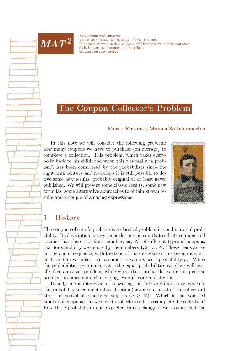
MAT 2 MATerialsMATemàtics Volum 2014, treball no. 2, 35 pp. ISSN: 1887-1097 Publicació electrònica de divulgació del Departament de Matemàtiques de la Universitat Autònoma de Barcelona www.mat.uab.cat/matmat The Coupon Collector’s Problem Marco Ferrante, Monica Saltalamacchia In this note we will consider the following problem: how many coupons we have to purchase (on average) to complete a collection. This problem, which takes every- body back to his childhood when this was really “a prob- lem”, has been considered by the probabilists since the eighteenth century and nowadays it is still possible to de- rive some new results, probably original or at least never published. We will present some classic results, some new formulas, some alternative approaches to obtain known re- sults and a couple of amazing expressions. 1 History The coupon collector’s problem is a classical problem in combinatorial prob- ability. Its description is easy: consider one person that collects coupons and assume that there is a finite number, say N , of different types of coupons, that for simplicity we denote by the numbers 1, 2,...,N . These items arrive one by one in sequence, with the type of the successive items being indepen- dent random variables that assume the value k with probability p k . When the probabilities p k are constant (the equal probabilities case) we will usu- ally face an easier problem, while when these probabilities are unequal the problem becomes more challenging, even if more realistic too. Usually one is interested in answering the following questions: which is the probability to complete the collection (or a given subset of the collection) after the arrival of exactly n coupons (n ≥ N )? Which is the expected number of coupons that we need to collect in order to complete the collection? How these probabilities and expected values change if we assume that the
-
Upload
phungquynh -
Category
Documents
-
view
241 -
download
0
Transcript of MATerials MATemàtics 2 - Departament de matemàtiquesmat.uab.cat/matmat/PDFv2014/v2014n02.pdf ·...
MAT 2MATerials MATemàticsVolum 2014, treball no. 2, 35 pp. ISSN: 1887-1097Publicació electrònica de divulgació del Departament de Matemàtiquesde la Universitat Autònoma de Barcelonawww.mat.uab.cat/matmat
The Coupon Collector’s Problem
Marco Ferrante, Monica Saltalamacchia
In this note we will consider the following problem:how many coupons we have to purchase (on average) tocomplete a collection. This problem, which takes every-body back to his childhood when this was really “a prob-lem”, has been considered by the probabilists since theeighteenth century and nowadays it is still possible to de-rive some new results, probably original or at least neverpublished. We will present some classic results, some newformulas, some alternative approaches to obtain known re-sults and a couple of amazing expressions.
1 HistoryThe coupon collector’s problem is a classical problem in combinatorial prob-ability. Its description is easy: consider one person that collects coupons andassume that there is a finite number, say N , of different types of coupons,that for simplicity we denote by the numbers 1, 2, . . . , N . These items arriveone by one in sequence, with the type of the successive items being indepen-dent random variables that assume the value k with probability pk. Whenthe probabilities pk are constant (the equal probabilities case) we will usu-ally face an easier problem, while when these probabilities are unequal theproblem becomes more challenging, even if more realistic too.
Usually one is interested in answering the following questions: which isthe probability to complete the collection (or a given subset of the collection)after the arrival of exactly n coupons (n ≥ N)? Which is the expectednumber of coupons that we need to collect in order to complete the collection?How these probabilities and expected values change if we assume that the
2 The Coupon Collector’s Problem
coupons arrive in groups of constant size or we are considering a group offriends that intends to complete m collections? In this note we will considerthe problem of more practical interest, which is the (average) number ofcoupons that one needs to purchase in order to complete one or more thanone collection in both the cases of equal and unequal probabilities. We willobtain explicit formulas for these expected values and, as suggested by theintuition, that the minimum expected number of purchases is needed in theequal case, while in the unequal case a very rare coupon can bring thisexpected number to tend to infinity.
We also present some approximation formulas for the results obtainedsince, most of all in the unequal probabilities case, even if the exact for-mulas appear easy and compact, they are computationally extraordinarilyheavy. Some of the results in this note are probably original or at least neverpublished before.
The history of the coupon collector’s problem began in 1708, when theproblem first appeared inDe Mensura Sortis (On the Measurement of Chance)written by A. De Moivre. More results, due among others to Laplace andEuler (see [8] for a comprehensive introduction on this topic), were obtainedin the case of constant probabilities, i.e. when pk ≡ 1
Nfor any k.
In 1954 H. Von Schelling [10] first obtained the waiting time to complete acollection when the probability of collecting each coupon wasn’t equal and in1960 D. J. Newman and L. Shepp [7] calculated the waiting time to completetwo collections of coupons in the equal case. More recently, some authorshave made further contribution to this classical problem (see e.g. L. Holst[4] and Flajolet et. al. [3]).
The coupon collector’s problem has many applications, especially in elec-trical engineering, where it is related to the cache fault problem and it can beused in electrical fault detection, and in biology, where it is used to estimatethe number of species of animals.
2 Single collection with equal probabilities
Assume that there are N different coupons and that they are equally likely,with the probability to purchase any type at any time equal to 1
N. In this
section we will derive the expected number of coupons that one needs topurchase in order to complete the collection. We will present two approaches,the first of which presents in most of the textbooks in Probability, and wederive a simple approximation of this value.
Marco Ferrante, Monica Saltalamacchia 3
2.1 The Geometric Distribution approach
Let X denote the (random) number of coupons that we need to purchase inorder to complete our collection. We can write X = X1 + X2 + . . . + XN ,where for any i = 1, 2, . . . , N , Xi denotes the additional number of couponsthat we need to purchase to pass from i − 1 to i different types of couponsin our collection. Trivially X1 = 1 and, since we are considering the caseof a uniform distribution, it follows that when i distinct types of couponshave been collected, a new coupon purchased will be of a distinct type withprobability equal to N−i
N. By the independence assumption, we get that
the random variable Xi, for i ∈ {2, . . . , N}, is independent from the othervariables and has a geometric law with parameter N−i+1
N. The expected
number of coupons that we have to buy to complete the collection will betherefore
E[X] = E[X1] + · · ·+ E[XN ]
= 1 +N
N − 1+
N
N − 2+ · · ·+ N
2+N
= NN∑i=1
1
i.
2.2 The Markov Chains approach
Even if the previous result is very simple and the formula completely clear,we will introduce an alternative approach, that we will use in the followingsections where the situation becomes more obscure. If we assume that onecoupon arrives at any unit of time, we can interpret the previous variablesXi as the additional time that we have to wait in order to collect the i-thcoupon after i− 1 different types of coupons have been collected. It is thenpossible to solve the previous problem by using a Markov Chains approach.
Let Yn be the number of different types of coupons collected after n unitsof time and assume again that the probability of finding a coupon of anytype at any time is p = 1
N. Yn will be clearly a Markov Chain on the state
space S = {0, 1, . . . , N} with |S| = N + 1 and it is immediate to obtain that
MAT 2MATerials MATematicsVolum 2006, treball no. 1, 14 pp.Publicacio electronica de divulgacio del Departament de Matematiquesde la Universitat Autonoma de Barcelonawww.mat.uab.cat/matmat
Trigonometria esferica i hiperbolicaJoan Girbau
L’objectiu d’aquestes notes es establir de forma curta i elegant les formulesfonamentals de la trigonometria esferica i de la trigonometria hiperbolica.La redaccio consta, doncs, de dues seccions independents, una dedicada a latrigonometria esferica i l’altra, a la hiperbolica. La primera esta adrecada aestudiants de primer curs de qualsevol carrera tecnica. La segona requereixdel lector coneixements rudimentaris de varietats de Riemann.
1 Trigonometria esferica
Aquells lectors que ja sapiguen que es un triangle esferic i com es mesuren elsseus costats i els seus angles poden saltar-se les subseccions 1.1 i 1.2 i passardirectament a la subseccio 1.3.
1.1 Arc de circumferencia determinat per dos punts
A cada dos punts A i B de la circumferencia unitat, no diametralment opo-sats, els hi associarem un unic arc de circumferencia, de longitud menor que!, (vegeu la figura 1) tal com explicarem a continuacio.
A
B
O
figura 1

4 The Coupon Collector’s Problem
its transition matrix is given by
P =
0 1 0 . . . . . . . . . 00 1
NN−1N
0 . . . . . . 00 0 2
NN−2N
0 . . . 0...
... . . . . . . . . . . . . ...0 . . . . . . . . . 0 N−1
N1N
0 . . . . . . . . . 0 0 1
.
Note that {N} is the unique closed class and the state N is absorbing. So, inorder to determine the mean time taken for Xn to reach the state N , which isequal to the expected number of coupons needed to complete the collection,we have to solve the linear system:kN = 0
ki = 1 +∑j 6=N
pijkj, i 6= N .
Using the transition matrix P , this system is equivalent to
k0 = k1 + 1
k1 = 1Nk1 + N−1
Nk2 + 1
k2 = 2Nk2 + N−2
Nk3 + 1
...kN−2 = N−2
NkN−2 + 2
NkN−1 + 1
kN−1 = N−1NkN−1 + 1
kN = 0
⇐⇒
kN = 01NkN−1 = 1
2NkN−2 = 2
NkN−1 + 1
...N−2Nk2 = N−2
Nk3 + 1
N−1Nk1 = N−1
Nk2 + 1
k0 = k1 + 1
⇐⇒
kN = 0
kN−1 = N
kN−2 = kN−1 + N2
= N + N2
kN−3 = kN2 + N3
= N + N2
+ N3
...k2 = k3 + N
N−2 = N + N2
+ · · ·+ NN−3 + N
N−2k1 = k2 + N
N−1 = N + N2
+ · · ·+ NN−2 + N
N−1k0 = k1 + 1 = N + N
2+ · · ·+ N
N−2 + NN−1 + 1
It follows that the waiting time to collect all N coupons is given by
k0 = NN∑i=1
1
i.
Marco Ferrante, Monica Saltalamacchia 5
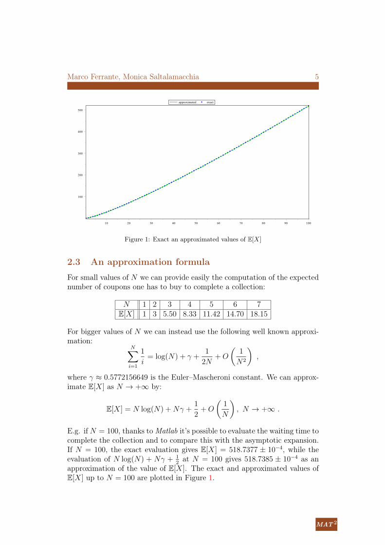
Figure 1: Exact an approximated values of E[X]
2.3 An approximation formula
For small values of N we can provide easily the computation of the expectednumber of coupons one has to buy to complete a collection:
N 1 2 3 4 5 6 7E[X] 1 3 5.50 8.33 11.42 14.70 18.15
For bigger values of N we can instead use the following well known approxi-mation:
N∑i=1
1
i= log(N) + γ +
1
2N+O
(1
N2
),
where γ ≈ 0.5772156649 is the Euler–Mascheroni constant. We can approx-imate E[X] as N → +∞ by:
E[X] = N log(N) +Nγ +1
2+O
(1
N
), N → +∞ .
E.g. if N = 100, thanks toMatlab it’s possible to evaluate the waiting time tocomplete the collection and to compare this with the asymptotic expansion.If N = 100, the exact evaluation gives E[X] = 518.7377 ± 10−4, while theevaluation of N log(N) + Nγ + 1
2at N = 100 gives 518.7385 ± 10−4 as an
approximation of the value of E[X]. The exact and approximated values ofE[X] up to N = 100 are plotted in Figure 1.
MAT 2MATerials MATematicsVolum 2006, treball no. 1, 14 pp.Publicacio electronica de divulgacio del Departament de Matematiquesde la Universitat Autonoma de Barcelonawww.mat.uab.cat/matmat
Trigonometria esferica i hiperbolicaJoan Girbau
L’objectiu d’aquestes notes es establir de forma curta i elegant les formulesfonamentals de la trigonometria esferica i de la trigonometria hiperbolica.La redaccio consta, doncs, de dues seccions independents, una dedicada a latrigonometria esferica i l’altra, a la hiperbolica. La primera esta adrecada aestudiants de primer curs de qualsevol carrera tecnica. La segona requereixdel lector coneixements rudimentaris de varietats de Riemann.
1 Trigonometria esferica
Aquells lectors que ja sapiguen que es un triangle esferic i com es mesuren elsseus costats i els seus angles poden saltar-se les subseccions 1.1 i 1.2 i passardirectament a la subseccio 1.3.
1.1 Arc de circumferencia determinat per dos punts
A cada dos punts A i B de la circumferencia unitat, no diametralment opo-sats, els hi associarem un unic arc de circumferencia, de longitud menor que!, (vegeu la figura 1) tal com explicarem a continuacio.
A
B
O
figura 1

6 The Coupon Collector’s Problem
Note that the exact computation in this case can be carried out up to bigvalues of N , but this will not be true in the case of unequal probabilities,that we will consider in the next section.
3 Single collection with unequal probabilities
Consider now the general case in which there are N different coupons and thetype of the successive items are independent random variables that assumethe value k with probability pk no more constant. Here we will have that the i-th coupon type can be purchased with probability pi ≥ 0, with p1+· · ·+pN =1. This is clearly the most realistic case, since in any collection there are “rare”coupons that makes the average number of coupons needed bigger and bigger.Our goal here is to find the expected number of coupons that we have to buyto complete the collection and we will recall a known formula (see e.g. Ross[8]), present a new formula (obtained in [2]) and a possible approximationprocedure, outlined in the case of the Mandelbrot distribution.
3.1 The Maximum-Minimums Identity approach
Let us now denote by Xi the random number of coupons we need to buy toobtain the first coupon of type i. The waiting time to complete the collectionis therefore given by the random variable X = max{X1, . . . , XN}. Note thatXi is a geometric random variable with parameter pi (because each newcoupon obtained is of type i with probability pi), but now these variablesare no more independent. Since the minimum of Xi and Xj is the numberof coupons needed to obtain either a coupon of type i or a coupon of typej, it follows that for i 6= j, min(Xi, Xj) is a geometric random variable withparameter pi + pj and the same holds true for the minimum of any finitenumber of these random variables. To compute the expected value of therandom variable X, we will use the Maximum-Minimums Identity, whose
Marco Ferrante, Monica Saltalamacchia 7
proof can be found e.g. in [8]:
E[X] = E[
maxi=1,...,N
Xi
]=∑i
E[Xi]−∑i<j
E[min(Xi, Xj)] +∑i<j<k
E[min(Xi, Xj, Xk)]− . . .
· · ·+ (−1)N+1E[min(X1, X2, . . . , XN)]
=∑i
1
pi−∑i<j
1
pi + pj+∑i<j<k
1
pi + pj + pk− . . .
· · ·+ (−1)N+1 1
p1 + · · ·+ pN.
Recalling that ∫ +∞
0
e−p x dx = − e−p x
p
∣∣∣∣x=+∞
x=0
=1
p
and integrating the identity
1−N∏i=1
(1− e−pi x) =∑i
e−pi x −∑i<j
e−(pi+pj)x + · · ·+ (−1)N+1e−(p1+···+pN )x
we get the useful equivalent expression:
E[X] =
∫ +∞
0
(1−
N∏i=1
(1− e−pi x)
)dx .
Remark 1. Let N be the number of different coupons we want to collectand assume that at each trial we find the i-th coupon with probability pi ≥ 0such that p1 + · · · + pN = 1. Our goal is to determine E[X], where X isthe number of coupons we have to buy in order to complete our collection.Assume that the number of coupons bought up to time t, say X(t), hasPoisson distribution with parameter λ = 1; let Yi be the generic interarrivaltime, which represents the time elapsed between the (i − 1)-th and the i-th purchase: Yi has exponential distribution with parameter λ = 1. Notethat X is independent from Yi for all i; indeed, knowing the time intervalbetween two subsequent purchases does not change the probability that thetotal number of purchases to complete the collection will be equal to a certainfixed value. Let Zi be the time in which the coupon of type i arrives for thefirst time (hence Zi ∼ exp(pi)) and let Z = max{Z1, . . . , ZN} be the time inwhich we have a coupon of each type (and so we complete the collection).
MAT 2MATerials MATematicsVolum 2006, treball no. 1, 14 pp.Publicacio electronica de divulgacio del Departament de Matematiquesde la Universitat Autonoma de Barcelonawww.mat.uab.cat/matmat
Trigonometria esferica i hiperbolicaJoan Girbau
L’objectiu d’aquestes notes es establir de forma curta i elegant les formulesfonamentals de la trigonometria esferica i de la trigonometria hiperbolica.La redaccio consta, doncs, de dues seccions independents, una dedicada a latrigonometria esferica i l’altra, a la hiperbolica. La primera esta adrecada aestudiants de primer curs de qualsevol carrera tecnica. La segona requereixdel lector coneixements rudimentaris de varietats de Riemann.
1 Trigonometria esferica
Aquells lectors que ja sapiguen que es un triangle esferic i com es mesuren elsseus costats i els seus angles poden saltar-se les subseccions 1.1 i 1.2 i passardirectament a la subseccio 1.3.
1.1 Arc de circumferencia determinat per dos punts
A cada dos punts A i B de la circumferencia unitat, no diametralment opo-sats, els hi associarem un unic arc de circumferencia, de longitud menor que!, (vegeu la figura 1) tal com explicarem a continuacio.
A
B
O
figura 1
8 The Coupon Collector’s Problem
Note that Z =∑N
i=0 Yi and E[X] = E[Z], indeed:
E[Z] = E[E[Z|X]] =∑k
E
[k∑i=1
Yi|X = k
]P(X = k)
=∑k
E
[k∑i=1
Yi
]P(X = k) =
∑k
k∑i=1
E[Yi]P(X = k)
=∑k
k P(X = k) = E[X] .
It follows that it suffices to calculate E[Z] to get E[X]. Since Z = max{Z1, ..,ZN}, we have:
FZ(t) = P(Z ≤ t) = P(Z1 ≤ t, . . . , ZN ≤ t) =N∏i=1
FZi(t) =
N∏i=1
(1− e−pi t)
and then
E[Z] =
∫ +∞
0
P(Z > t) dt =
∫ +∞
0
(1−
N∏i=1
(1− e−pi t)
)dt .
3.2 An alternative approach
In [2] has been observed that the coupon collector’s problem is related to thefollowing more general problem: given a discrete distribution, determine theminimum size of a random sample drawn from that distribution, in order toobserve a given number of different records. The expected size of such a sam-ple can be seen as an alternative method to compute the expected numberof coupons needed to complete a collection.Let S = {1, . . . , N} be the support of a given discrete distribution, p =(p1, . . . , pN) its discrete density and assume that the elements are drawnrandomly from this distribution in sequence; the random variables in thesample will be independent and the realization of each of these will be equalto k with probability pk. Our aim is to compute the number of drawn oneneeds to obtain k different realizations of the given distribution. Let X1 bethe random number of drawn needed to have the first record, let X2 be thenumber of additional drawn needed to obtain the second record and in gen-eral let Xi be the number of drawn needed to go from the (i − 1)-th to thei-th different record in the sample for every i ≤ N .It follows that the random number XN(k) of drawn one needs to obtain kdifferent records is equal to X1 + · · ·+Xk and P(XN(k) < +∞) = 1.
Marco Ferrante, Monica Saltalamacchia 9
Note that this problem is very close to the classical coupon collector’s prob-lem, but in that case the random variables Xi denote the number of couponsone has to buy to go from the (i− 1)-th to the i-th different type of couponin the collection and XN(N) represents the number of coupons one has tobuy to complete the collection.In the case of uniform distribution, i.e. pk = 1
Nfor any k ∈ {1, . . . , N},
the random variable Xi, for i ∈ {2, . . . , N}, has geometric law with param-eter N−i
N, hence the expected number of drawn needed to obtain k different
records is given by:
E[XN(k)] = 1 +N
N − 1+
N
N − 2+ · · ·+ N
N − k + 1.
Note that if k = N we obtain the solution of the coupon collector’s problemin the case of uniform distribution. When the probabilities pk are unequal,to compute the expected value of the random variables Xi we have firstto compute their expected values given the types of the preceding i − 1different records obtained. To simplify the notation, define p(i1, . . . , ik) =1 − pi1 − · · · − pik for k ≤ N and different indexes i1, i2, . . . , ik. It can beproved that:
Proposition 1. For any k ∈ {2, . . . , N}, the expected value of Xk is givenby:
E[Xk] =N∑
i1 6=i2 6=···6=ik−1=1
pi1 . . . pik−1
p(i1) p(i1, i2) . . . p(i1, i2, . . . , ik−1)
and therefore:
E[XN(k)] =k∑s=1
E[Xs]
= 1 +N∑i1=1
pi1p(i1)
+N∑
i1 6=i2=1
pi1 pi2p(i1) p(i1, i2)
+ . . . (1)
· · ·+N∑
i1 6=i2 6=···6=ik−1=1
pi1 . . . pik−1
p(i1) p(i1, i2) . . . p(i1, i2, . . . , ik−1).
Remark 2. Note that, when k = N , the last expression represents an alter-native way to compute the expected number of coupons needed to completea collection. The proof of the equivalence between the last expression withk = N and the formula obtained using the Maximum-Minimums Identity isnot trivial; furthermore, both expressions are not computable for large valuesof k.
MAT 2MATerials MATematicsVolum 2006, treball no. 1, 14 pp.Publicacio electronica de divulgacio del Departament de Matematiquesde la Universitat Autonoma de Barcelonawww.mat.uab.cat/matmat
Trigonometria esferica i hiperbolicaJoan Girbau
L’objectiu d’aquestes notes es establir de forma curta i elegant les formulesfonamentals de la trigonometria esferica i de la trigonometria hiperbolica.La redaccio consta, doncs, de dues seccions independents, una dedicada a latrigonometria esferica i l’altra, a la hiperbolica. La primera esta adrecada aestudiants de primer curs de qualsevol carrera tecnica. La segona requereixdel lector coneixements rudimentaris de varietats de Riemann.
1 Trigonometria esferica
Aquells lectors que ja sapiguen que es un triangle esferic i com es mesuren elsseus costats i els seus angles poden saltar-se les subseccions 1.1 i 1.2 i passardirectament a la subseccio 1.3.
1.1 Arc de circumferencia determinat per dos punts
A cada dos punts A i B de la circumferencia unitat, no diametralment opo-sats, els hi associarem un unic arc de circumferencia, de longitud menor que!, (vegeu la figura 1) tal com explicarem a continuacio.
A
B
O
figura 1
10 The Coupon Collector’s Problem
Proof of Proposition 1: In order to compute the expected value of thevariable Xk, we shall take the expectation of the conditional expectation ofXk given Z1, . . . , Zk−1, where Zi, for i = 1, . . . , N , denotes the type of thei-th different coupon collected.To simplify the exposition, let us start by evaluating E[X2]; we have imme-diately that X2|Z1 = i has a (conditioned) geometric law with parameter1− pi = p(i) and therefore E[X2|Z1 = i] = 1
p(i). So
E[X2] = E[E[X2|Z1]] =N∑i=1
E[X2|Z1 = i]P[Z1 = i] =N∑i=1
pip(i)
.
Let us now take k ∈ {3, . . . , N}: it is easy to see that
E[Xk] = E[E[Xk|Z1, Z2, . . . , Zk−1]]
=N∑
i1 6=i2 6=···6=ik−1=1
E[Xk|Z1 = i1, , Z2 = i2, · · · , Zk−1 = ik−1]
× P[Z1 = i1, ..., Zk−1 = ik−1] .
Note that P[Zi = Zj] = 0 for any i 6= j. The conditional law of Xk|Z1 =i1, Z2 = i2, · · · , Zk−1 = ik−1, for i1 6= i2 6= · · · 6= ik−1, is that of a geometricrandom variable with parameter p(i1, . . . , ik−1) and its conditional expecta-tion is p(i1, . . . , ik−1)−1. By the multiplication rule, we get
P[Z1 = i1, ..., Zk−1 = ik−1] = P[Z1 = i1]× P[Z2 = i2|Z1 = i1]×· · · × P[Zk−1 = ik−1|Z1 = i1, . . . , Zk−2 = ik−2] .
Note that, even though the types of the successive coupons are independentrandom variables, the random variables Zi are not mutually independent. Asimple computation gives, for any s = 2, . . . , k − 1, that
P[Zs = is|Z1 = i1, . . . , Zs−1 = is−1] =pis
1− pi1 − . . .− pis−1
if i1 6= i2 6= · · · 6= ik−1 and zero otherwise. Recalling the compact notationp(i1, . . . , ik) = 1− pi1 − . . .− pik , we then get
E[Xk] =N∑
i1 6=i2 6=···6=ik−1=1
pi1 pi2 · · · pik−1
p(i1) p(i1, i2) · · · p(i1, i2, . . . , ik−1)
and the proof is complete.
Marco Ferrante, Monica Saltalamacchia 11
3.3 An approximation procedure via the Heaps’ law innatural languages
In [2] Ferrante and Frigo proposed the following procedure in order to ap-proximate the expected number of coupons needed to complete a collectionin the unequal case.
Let us consider a text written in a natural language: the Heaps’ law is anempirical law which describes the portion of the vocabulary which is used inthe given text. This law can be described by the following formula
E[Rm(n)] ∼ K nβ
where Rm(n) is the (random) number of different words presents in a textconsisting of n words and taken from a vocabulary of m words, while K andβ are free parameters determined empirically. In order to obtain a formalderivation of this empirical law, van Leijenhorst and van der Weide in [5] haveconsidered the average growth in the number of records, when elements aredrawn randomly from some statistical distribution that can assume exactlym different values. The exact computation of the average number of recordsin a sample of size n, E[Rm(n)], can be easily obtained using the followingapproach. Let S = {1, 2, . . . ,m} be the support of the given distribution,define X = m − Rm(n) the number of values in S not observed and denoteby Ai the event that the record i is not observed. It is immediate to see thatP[Ai] = (1− pi)n, X =
∑mi=1 1Ai
and therefore that
E[Rm(n)] = m− E[X] = m−m∑i=1
(1− pi)n . (2)
Assuming now that the elements are drawn randomly from the Mandelbrotdistribution, van Leijenhorst and van der Weide obtain that the Heaps’ lawis asymptotically true as n and m go to infinity and n � mθ−1, where θ isone of the parameters of the Mandelbrot distribution (see [5] for the details).
It is possible to relate this problem with the previous one: assume thatwe are interested in the minimum number Xm(k) of elements that we haveto draw randomly from a given statistical distribution in order to obtaink different records. This is clearly strictly related to the previous problemand at first sight one expects that the technical difficulties would be similar.However, we have just proved that the computation of the expectation ofXm(k) is much more complicated. The formula that we obtained before iscomputationally hard and we are able to perform the exact computation inthe environment R just for distributions with a support of small cardinal-ity. An approximation procedure can be obtained in the special case of the
MAT 2MATerials MATematicsVolum 2006, treball no. 1, 14 pp.Publicacio electronica de divulgacio del Departament de Matematiquesde la Universitat Autonoma de Barcelonawww.mat.uab.cat/matmat
Trigonometria esferica i hiperbolicaJoan Girbau
L’objectiu d’aquestes notes es establir de forma curta i elegant les formulesfonamentals de la trigonometria esferica i de la trigonometria hiperbolica.La redaccio consta, doncs, de dues seccions independents, una dedicada a latrigonometria esferica i l’altra, a la hiperbolica. La primera esta adrecada aestudiants de primer curs de qualsevol carrera tecnica. La segona requereixdel lector coneixements rudimentaris de varietats de Riemann.
1 Trigonometria esferica
Aquells lectors que ja sapiguen que es un triangle esferic i com es mesuren elsseus costats i els seus angles poden saltar-se les subseccions 1.1 i 1.2 i passardirectament a la subseccio 1.3.
1.1 Arc de circumferencia determinat per dos punts
A cada dos punts A i B de la circumferencia unitat, no diametralment opo-sats, els hi associarem un unic arc de circumferencia, de longitud menor que!, (vegeu la figura 1) tal com explicarem a continuacio.
A
B
O
figura 1
12 The Coupon Collector’s Problem
Mandelbrot distribution, widely used in the applications, making use of theasymptotic results proved in [5] in order to derive the Heaps’ law.
The exact formula we obtained in the previous section is nice, but it istremendously heavy to compute as soon as the cardinality of the support ofthe distribution becomes larger then 10. The number of all possible orderedchoices of indexes sets involved in (1) increases very fast with k leadingthe objects hard to handle with a personal computer. For this reason itwould be important to be able to approximate this formula, at least in somecases of interest, even if its complicated structure may suggest that it couldbe quite difficult in general. In this section we shall consider the case ofthe Mandelbrot distribution, which is commonly used in the Heaps’ law andother practical problems. Applying the results proved in [5], we present here apossible strategy to approximate the expectation of Xm(k) and present somenumerical approximation in order to test our procedure. Let us considerRm(n) and Xm(k): these two random variables are strictly related, since[Rm(n) > k] = [Xm(k) < n], for k ≤ n ≤ m. However, we have seenthat the computation of their expected values is quite different. With anabuse of language, we could say that the two functions n 7→ E[Rm(n)] andk 7→ E[Xm(k)] represent one the “inverse” of the other. In order to confirmthis statement, let us consider the case studied in [5], i.e. let us assume tosample from the Mandelbrot distribution. Fixed three parameters m ∈ N,θ ∈ [1, 2] and c ≥ 0, we shall assume that S = {1, . . . ,m} and
pi = am(c+ i)−θ , am =
(m∑i=1
(c+ i)−θ
)−1. (3)
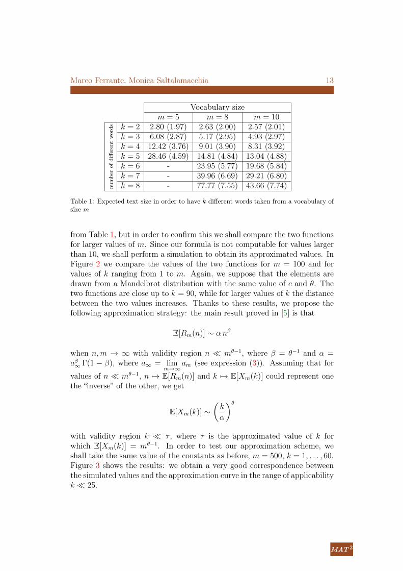
We implement both the expressions (2) and (1) using the environment R.We set the parameters of the Mandelbrot distribution to be c = 0.30 andθ = 1.75. Using (1), we compute the expected number E[Xm(k)] of elementswe have to draw randomly from a Mandelbrot distribution in order to obtaink different records, for three levels of m, being m the vocabulary size, i.e themaximum size of different words. In brackets we show the expected numberof different words in a random selection of exactly E[Xm(k)] elements, com-puted using (2). Results are collected in Table 1. We see that the numberof different words we expect in a text size of dimension E[Xm(k)] is closeto the value of k and this supports our statement about the connection be-tween E[Rm(n)] and E[Xm(k)]. As underlined before, we can compute theseexpectations only for small values of k.
At the same time, since E[Rm(n)] ≤ m, it is clear that our statement thatn 7→ E[Rm(n)] and k 7→ E[Xm(k)] represent one the “inverse” of the othercould be valid just for values of k small with respect tom. This idea arises also
Marco Ferrante, Monica Saltalamacchia 13
Vocabulary sizem = 5 m = 8 m = 10
numbe
rof
diffe
rent
words k = 2 2.80 (1.97) 2.63 (2.00) 2.57 (2.01)
k = 3 6.08 (2.87) 5.17 (2.95) 4.93 (2.97)k = 4 12.42 (3.76) 9.01 (3.90) 8.31 (3.92)k = 5 28.46 (4.59) 14.81 (4.84) 13.04 (4.88)k = 6 - 23.95 (5.77) 19.68 (5.84)k = 7 - 39.96 (6.69) 29.21 (6.80)k = 8 - 77.77 (7.55) 43.66 (7.74)
Table 1: Expected text size in order to have k different words taken from a vocabulary ofsize m
from Table 1, but in order to confirm this we shall compare the two functionsfor larger values of m. Since our formula is not computable for values largerthan 10, we shall perform a simulation to obtain its approximated values. InFigure 2 we compare the values of the two functions for m = 100 and forvalues of k ranging from 1 to m. Again, we suppose that the elements aredrawn from a Mandelbrot distribution with the same value of c and θ. Thetwo functions are close up to k = 90, while for larger values of k the distancebetween the two values increases. Thanks to these results, we propose thefollowing approximation strategy: the main result proved in [5] is that
E[Rm(n)] ∼ αnβ
when n,m → ∞ with validity region n � mθ−1, where β = θ−1 and α =aβ∞ Γ(1 − β), where a∞ = lim
m→∞am (see expression (3)). Assuming that for
values of n � mθ−1, n 7→ E[Rm(n)] and k 7→ E[Xm(k)] could represent onethe “inverse” of the other, we get
E[Xm(k)] ∼(k
α
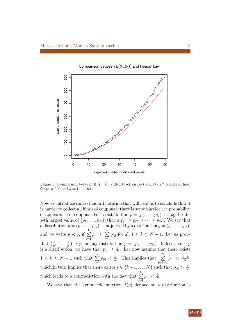
)θwith validity region k � τ , where τ is the approximated value of k forwhich E[Xm(k)] = mθ−1. In order to test our approximation scheme, weshall take the same value of the constants as before, m = 500, k = 1, . . . , 60.Figure 3 shows the results: we obtain a very good correspondence betweenthe simulated values and the approximation curve in the range of applicabilityk � 25.
MAT 2MATerials MATematicsVolum 2006, treball no. 1, 14 pp.Publicacio electronica de divulgacio del Departament de Matematiquesde la Universitat Autonoma de Barcelonawww.mat.uab.cat/matmat
Trigonometria esferica i hiperbolicaJoan Girbau
L’objectiu d’aquestes notes es establir de forma curta i elegant les formulesfonamentals de la trigonometria esferica i de la trigonometria hiperbolica.La redaccio consta, doncs, de dues seccions independents, una dedicada a latrigonometria esferica i l’altra, a la hiperbolica. La primera esta adrecada aestudiants de primer curs de qualsevol carrera tecnica. La segona requereixdel lector coneixements rudimentaris de varietats de Riemann.
1 Trigonometria esferica
Aquells lectors que ja sapiguen que es un triangle esferic i com es mesuren elsseus costats i els seus angles poden saltar-se les subseccions 1.1 i 1.2 i passardirectament a la subseccio 1.3.
1.1 Arc de circumferencia determinat per dos punts
A cada dos punts A i B de la circumferencia unitat, no diametralment opo-sats, els hi associarem un unic arc de circumferencia, de longitud menor que!, (vegeu la figura 1) tal com explicarem a continuacio.
A
B
O
figura 1

14 The Coupon Collector’s Problem
0 20 40 60 80 100
050
0015
000
Comparison between E(Xm(k)) and E(Rm(n))
expected number of different words
size
of r
ando
m s
elec
tion
0 20 40 60 80
010
0020
00
expected number of different words
size
of r
ando
m s
elec
tion
85 90 95 100
4000
8000
1400
0
expected number of different words
size
of r
ando
m s
elec
tion
Figure 2: Comparison between E[Xm(k)] (filled red circles) and E[Rm(n)] (solid black cir-cles) for m = 100 and k = 1, . . . , 100 (main figure). Zoom: comparison between E[Xm(k)](solid red line) and E[Rm(n)] (dashed black line) for k = 1, . . . , 80 (left) and k = 81, . . . , 100(right).
3.4 Comparison between the equal and unequal cases
Let us denote by X( 1N,..., 1
N ) the random number of coupons we have to buy tocomplete the collection using the uniform probability and by X(p1,...,pN ) thenumber of coupons in the unequal case. We have already calculated theirexpectations:
E[X( 1N,..., 1
N )] = NN∑i=1
1
i,
E[X(p1,...,pN )] =∑i
1
pi−∑i<j
1
pi + pj+ · · ·+ (−1)N+1 1
p1 + · · ·+ pN.
Marco Ferrante, Monica Saltalamacchia 15
0 10 20 30 40 50 60
010
020
030
040
050
060
0Comparison between E(Xm(k)) and Heaps’ Law
expected number of different words
size
of r
ando
m s
elec
tion
Figure 3: Comparison between E[Xm(k)] (filled black circles) and (k/α)θ (solid red line)for m = 500 and k = 1, . . . , 60.
Now we introduce some standard notation that will lead us to conclude that itis harder to collect all kinds of coupons if there is some bias for the probabilityof appearance of coupons. For a distribution p = (p1, . . . , pN), let p[j] be thej-th largest value of {p1, . . . , pN}, that is p[1] ≥ p[2] ≥ · · · ≥ p[N ]. We say thata distribution p = (p1, . . . , pN) is majorized by a distribution q = (q1, . . . , qN),
and we write p ≺ q, ifk∑i=1
p[i] ≤k∑j=1
q[j] for all 1 ≤ k ≤ N − 1. Let us prove
that(
1N, . . . , 1
N
)≺ p for any distribution p = (p1, . . . , pN). Indeed, since p
is a distribution, we have that p[1] ≥ 1N. Let now assume that there exists
1 < k ≤ N − 1 such thatk∑i=1
p[i] <kN. This implies that
N∑i=k+1
p[i] >N−kN
,
which in turn implies that there exists j ∈ {k+1, . . . , N} such that p[j] > 1N,
which leads to a contradiction with the fact thatk∑i=1
p[i] <kN.
We say that the symmetric function f(p) defined on a distribution is
MAT 2MATerials MATematicsVolum 2006, treball no. 1, 14 pp.Publicacio electronica de divulgacio del Departament de Matematiquesde la Universitat Autonoma de Barcelonawww.mat.uab.cat/matmat
Trigonometria esferica i hiperbolicaJoan Girbau
L’objectiu d’aquestes notes es establir de forma curta i elegant les formulesfonamentals de la trigonometria esferica i de la trigonometria hiperbolica.La redaccio consta, doncs, de dues seccions independents, una dedicada a latrigonometria esferica i l’altra, a la hiperbolica. La primera esta adrecada aestudiants de primer curs de qualsevol carrera tecnica. La segona requereixdel lector coneixements rudimentaris de varietats de Riemann.
1 Trigonometria esferica
Aquells lectors que ja sapiguen que es un triangle esferic i com es mesuren elsseus costats i els seus angles poden saltar-se les subseccions 1.1 i 1.2 i passardirectament a la subseccio 1.3.
1.1 Arc de circumferencia determinat per dos punts
A cada dos punts A i B de la circumferencia unitat, no diametralment opo-sats, els hi associarem un unic arc de circumferencia, de longitud menor que!, (vegeu la figura 1) tal com explicarem a continuacio.
A
B
O
figura 1
16 The Coupon Collector’s Problem
Schur convex (resp. concave) if p ≺ q =⇒ f(p) ≤ f(q) (resp. f(p) ≥ f(q)).Finally, we say that a random variable X is stochastically smaller than arandom variable Y if P(X > a) ≤ P(Y > a) for all real a. The followingresults have been proved in [6]:
Theorem 1. The probability P(Xp ≤ n) is a Schur concave function of p.
Corollary 1. If p ≺ q, then Xp is stochastically smaller than Xq. In partic-ular: X( 1
N,..., 1
N ) is stochastically smaller than Xp for all p.
Corollary 2. The expectation E[Xp] is a Schur convex function of p. Inparticular: E[X( 1
N,..., 1
N )] ≤ E[X(p1,...,pN )] for all p.
3.5 Examples
• N = 2, E[X( 12, 12)] = 3
◦ p1 = 13, p2 = 2
3
E[X(p1,p2)] =1
p1+
1
p2− 1
p1 + p2= 3 +
3
2− 1 =
7
2= 3.5
◦ p1 = 16, p2 = 5
6
E[X(p1,p2)] =1
p1+
1
p2− 1
p1 + p2= 6 +
6
5− 1 =
31
5= 6.2
• N = 3, E[X( 13, 13, 13)] = 5.5
◦ p1 = 14, p2 = 1
2, p3 = 1
4
E[X(p1,p2,p3)] =1
p1+
1
p2− 1
p1 + p2− 1
p1 + p3− 1
p2 + p3
+1
p1 + p2 + p3=
19
3≈ 6.33
◦ p1 = 16, p2 = 4
6, p3 = 1
6
E[X(p1,p2,p3)] =1
p1+
1
p2− 1
p1 + p2− 1
p1 + p3− 1
p2 + p3
+1
p1 + p2 + p3=
91
10= 9.1 .
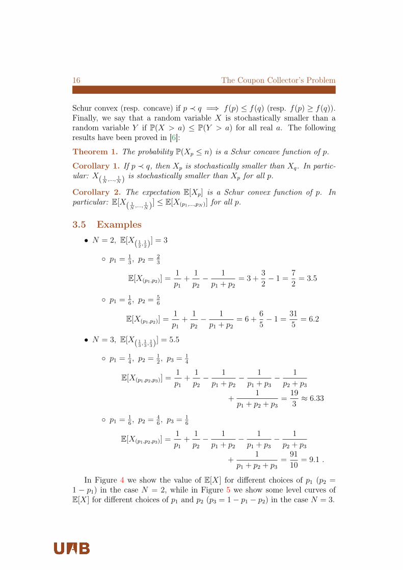
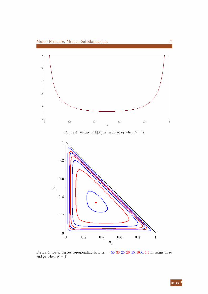
In Figure 4 we show the value of E[X] for different choices of p1 (p2 =1 − p1) in the case N = 2, while in Figure 5 we show some level curves ofE[X] for different choices of p1 and p2 (p3 = 1− p1 − p2) in the case N = 3.
Marco Ferrante, Monica Saltalamacchia 17
Figure 4: Values of E[X] in terms of p1 when N = 2
Figure 5: Level curves coresponding to E[X] = 50, 30, 25, 20, 15, 10, 6, 5.5 in terms of p1and p2 when N = 3
MAT 2MATerials MATematicsVolum 2006, treball no. 1, 14 pp.Publicacio electronica de divulgacio del Departament de Matematiquesde la Universitat Autonoma de Barcelonawww.mat.uab.cat/matmat
Trigonometria esferica i hiperbolicaJoan Girbau
L’objectiu d’aquestes notes es establir de forma curta i elegant les formulesfonamentals de la trigonometria esferica i de la trigonometria hiperbolica.La redaccio consta, doncs, de dues seccions independents, una dedicada a latrigonometria esferica i l’altra, a la hiperbolica. La primera esta adrecada aestudiants de primer curs de qualsevol carrera tecnica. La segona requereixdel lector coneixements rudimentaris de varietats de Riemann.
1 Trigonometria esferica
Aquells lectors que ja sapiguen que es un triangle esferic i com es mesuren elsseus costats i els seus angles poden saltar-se les subseccions 1.1 i 1.2 i passardirectament a la subseccio 1.3.
1.1 Arc de circumferencia determinat per dos punts
A cada dos punts A i B de la circumferencia unitat, no diametralment opo-sats, els hi associarem un unic arc de circumferencia, de longitud menor que!, (vegeu la figura 1) tal com explicarem a continuacio.
A
B
O
figura 1
18 The Coupon Collector’s Problem
4 Coupons in groups of constant sizeConsider now the case of coupons which arrives in groups of constant size g,with 1 < g < N , independently and with unequal probabilities; assume thateach group does not contain more than one coupon of any type, hence thetotal number of groups will be
(Ng
)and each group A can be identified with
a vector (a1, . . . , ag) ∈ {1, . . . , N}g with ai < ai+1 for i = 1, . . . , g − 1.Moreover, assume that the type of successive groups of coupons that onecollects form a sequence of independent random variables.
To study the unequal probabilities case, we first order the groups accord-ing to the lexicographical order (i.e. A = (a1, . . . , ag) < B = (b1, . . . , bg) ifthere exists i ∈ {1, . . . , g − 1} such that as = bs for s < i and ai < bi).We denote by qi, i ∈
{1, . . . ,
(Ng
)}, the probability to purchase (at any given
time) the i-th group of coupons, according to the lexicographical order, andgiven k ∈ {1, . . . , N−g} we denote by q(i1, . . . , ik) the probability to purchasea group of coupons which does not contain any of the coupons i1, . . . , ik.
To compute the probabilities q(i1, . . . , ik)’s, note that by the defined or-dering it holds that:
q(1) =
(Ng )∑
i=(N−1g−1)+1
qi , q(2) =
(Ng )∑
i=(N−1g−1)+(N−2
g−1)+1
qi
and in general:
q(1, 2, . . . , k) =
(Ng )∑
i=(N−1g−1)+···+(N−k
g−1 )+1
qi, if k ≤ N − g
0 otherwise.
For any permutation (i1, . . . , iN) of (1, . . . , N), one first reorders the qi’saccording to the lexicographical order of this new alphabet and then compute
q(i1, i2, . . . , ik) =
(Ng )∑
i=(N−1g−1)+···+(N−k
g−1 )+1
qi, if k ≤ N − g
0 otherwise.
Marco Ferrante, Monica Saltalamacchia 19
Remark 3. There are many conceivable choices for the unequal probabili-ties qi’s. For example, we can assume that one forms the groups followingthe strategy of the draft lottery in the American professional sports, wheredifferent proportion of the different coupons are put together and we chooseat random in sequence the coupons, discarding the eventually duplicates, upto obtaining a group of k coupons. Or, more simply, we can assume that thei-th coupon will arrive with probability pi and that the probability of anygroup is proportional to the product of the probabilities of the single couponscontained.
Let us start with the case of uniform probabilities, i.e.
qi =1(Ng
)
for any i, and let us define the following set of random variables:
Vi = {number of groups to purchase to obtain the first coupon of type i}.
These random variables have a geometric law with parameter
1−(N−1g
)(Ng
) ,
therefore the random variables min(Vi, Vj) have geometric law with param-
eter 1 − (N−2g )
(Ng )
and the random variables min(Vi1 , . . . , ViN−g) have geometric
law with parameter 1 − 1
(Ng ); the minimum of more random variables, i.e.
min(Vi1 , . . . , Vik) for k > N − g + 1, will be equal to the constant randomvariable 1. Applying the Maximum-Minimums Principle, we obtain the ex-pected number of groups of coupons that we have to buy to complete the
MAT 2MATerials MATematicsVolum 2006, treball no. 1, 14 pp.Publicacio electronica de divulgacio del Departament de Matematiquesde la Universitat Autonoma de Barcelonawww.mat.uab.cat/matmat
Trigonometria esferica i hiperbolicaJoan Girbau
L’objectiu d’aquestes notes es establir de forma curta i elegant les formulesfonamentals de la trigonometria esferica i de la trigonometria hiperbolica.La redaccio consta, doncs, de dues seccions independents, una dedicada a latrigonometria esferica i l’altra, a la hiperbolica. La primera esta adrecada aestudiants de primer curs de qualsevol carrera tecnica. La segona requereixdel lector coneixements rudimentaris de varietats de Riemann.
1 Trigonometria esferica
Aquells lectors que ja sapiguen que es un triangle esferic i com es mesuren elsseus costats i els seus angles poden saltar-se les subseccions 1.1 i 1.2 i passardirectament a la subseccio 1.3.
1.1 Arc de circumferencia determinat per dos punts
A cada dos punts A i B de la circumferencia unitat, no diametralment opo-sats, els hi associarem un unic arc de circumferencia, de longitud menor que!, (vegeu la figura 1) tal com explicarem a continuacio.
A
B
O
figura 1
20 The Coupon Collector’s Problem
collection:
E[max(V1, . . . , VN)] =∑
1≤i≤N
E[Vi]−∑
1≤i≤j≤N
E[min(Vi, Vj)] + . . .
· · ·+ (−1)N−g+1∑
0≤i1<i2<···<iN−g≤N
E[Vi1 , . . . , ViN−g+1]
+ (−1)N−g+2∑
0≤i1<i2<···<iN−g+1≤N
1 + · · ·+ (−1)N+1
=
(N
1
)1
1− (N−1g )
(Ng )
−(N
2
)1
1− (N−2g )
(Ng )
+
(N
3
)1
1− (N−3g )
(Ng )
− . . .
· · ·+ (−1)N−g+1
(N
N − g
)1
1− 1
(Ng )
+∑
1≤k≤g
(−1)N−g+k+1
(N
N − g + k
).
This result has been first proved byW. Stadje in [9] with a different technique,but with the present approach developed in [1] it can be easily generalizedto the unequal probabilities case as follows:
Proposition 2. The expected number of groups of coupons that we need tocomplete the collection, in the case of unequal probabilities qi, is equal to:
∑1≤i≤N
1
1− q(i)−
∑1≤i≤j≤N
1
1− q(i, j)+
∑0≤i<j<l≤N
1
1− q(i, j, l)− . . .
· · ·+ (−1)N−g+1∑
0≤i1<i2<···<iN−g≤N
1
1− q(i1, . . . , iN−g)
+∑
1≤k≤g
(−1)N−g+k+1
(N
N − g + k
).
In the following Table we list the mean number of groups of coupons ofconstant size g that we have to buy to complete a collection of N coupons
Marco Ferrante, Monica Saltalamacchia 21
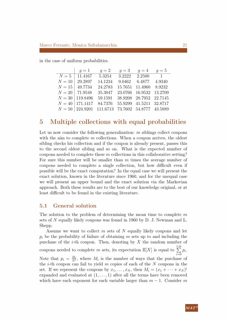
in the case of uniform probabilities.
g = 1 g = 2 g = 3 g = 4 g = 5N = 5 11.4167 5.3254 3.2222 2.2500 1N = 10 29.2897 14.1234 9.0462 6.4877 4.9340N = 15 49.7734 24.2783 15.7651 11.4960 8.9232N = 20 71.9548 35.3047 23.0766 16.9532 13.2709N = 30 119.8496 59.1591 38.9208 28.7952 22.7145N = 40 171.1417 84.7376 55.9299 41.5211 32.8717N = 50 224.9201 111.6713 73.7602 54.8777 43.5889
5 Multiple collections with equal probabilitiesLet us now consider the following generalization: m siblings collect couponswith the aim to complete m collections. When a coupon arrives, the oldestsibling checks his collection and if the coupon is already present, passes thisto the second oldest sibling and so on. What is the expected number ofcoupons needed to complete these m collections in this collaborative setting?For sure this number will be smaller than m times the average number ofcoupons needed to complete a single collection, but how difficult even ifpossible will be the exact computation? In the equal case we will present theexact solution, known in the literature since 1960, and for the unequal casewe will present an upper bound and the exact solution via the Markovianapproach. Both these results are to the best of our knowledge original, or atleast difficult to be found in the existing literature.
5.1 General solution
The solution to the problem of determining the mean time to complete msets of N equally likely coupons was found in 1960 by D. J. Newman and L.Shepp.
Assume we want to collect m sets of N equally likely coupons and letpi be the probability of failure of obtaining m sets up to and including thepurchase of the i-th coupon. Then, denoting by X the random number of
coupons needed to complete m sets, its expectation E[X] is equal to+∞∑i=0
pi.
Note that pi = Mi
N i , where Mi is the number of ways that the purchase ofthe i-th coupon can fail to yield m copies of each of the N coupons in theset. If we represent the coupons by x1, . . . , xN , then Mi = (x1 + · · · + xN)i
expanded and evaluated at (1, . . . , 1) after all the terms have been removedwhich have each exponent for each variable larger than m − 1. Consider m
MAT 2MATerials MATematicsVolum 2006, treball no. 1, 14 pp.Publicacio electronica de divulgacio del Departament de Matematiquesde la Universitat Autonoma de Barcelonawww.mat.uab.cat/matmat
Trigonometria esferica i hiperbolicaJoan Girbau
L’objectiu d’aquestes notes es establir de forma curta i elegant les formulesfonamentals de la trigonometria esferica i de la trigonometria hiperbolica.La redaccio consta, doncs, de dues seccions independents, una dedicada a latrigonometria esferica i l’altra, a la hiperbolica. La primera esta adrecada aestudiants de primer curs de qualsevol carrera tecnica. La segona requereixdel lector coneixements rudimentaris de varietats de Riemann.
1 Trigonometria esferica
Aquells lectors que ja sapiguen que es un triangle esferic i com es mesuren elsseus costats i els seus angles poden saltar-se les subseccions 1.1 i 1.2 i passardirectament a la subseccio 1.3.
1.1 Arc de circumferencia determinat per dos punts
A cada dos punts A i B de la circumferencia unitat, no diametralment opo-sats, els hi associarem un unic arc de circumferencia, de longitud menor que!, (vegeu la figura 1) tal com explicarem a continuacio.
A
B
O
figura 1
22 The Coupon Collector’s Problem
fixed and introduce the following notation: if P (x1, . . . , xN) is a polynomial(or a power series) we define {P (x1, . . . , xN)} to be the polynomial (or series)resulting when all terms having all exponents greater or equal to m havebeen removed. In terms of this notation, pi equals to {(x1+···+xN )i}
N i evaluatedat x1 = · · · = xN = 1. Define
Sm(t) =m−1∑k=0
tk
k!
and consider the expression
F = ex1+···+xN − (ex1 − Sm(x1))× · · · × (exN − Sm(xN)) .
Note that F has no terms with all exponents greater or equal to m, but Fdoesn’t have all terms of ex1+···+xN with at least one exponent smaller thanm; it follows that
F = {ex1+···+xN} =∞∑i=0
{(x1 + · · ·+ xN)i}i!
.
Remembering that
E[X] =∞∑i=0
pi =∞∑i=0
{(x1 + · · ·+ xN)i}N i
at x1 = · · · = xN = 1, and using the identity
N
∫ +∞
0
ti
i!e−Nt dt =
1
N i
it follows that∞∑i=0
{(x1 + · · ·+ xN)i}N i
=∞∑i=0
({(x1 + · · ·+ xN)i}N
∫ +∞
0
ti
i!e−N t dt
)= N
∫ +∞
0
∞∑i=0
({(x1 + · · ·+ xN)i} t
i
i!
)e−N t dt
= N
∫ +∞
0
[et (x1+···+xN ) −
(et x1 − Sm(t x1)
)× . . .
· · · ×(et xN − Sm(t xN)
)]e−N t dt .
Marco Ferrante, Monica Saltalamacchia 23
We easily obtain, evaluating the previous expressions for x1 = · · · = xN = 1,
E[X] = N
∫ +∞
0
[1−
(1− Sm(t) e−t
)N]dt .
So in order to determine the explicit value, we have to substitute the corre-sponding value of Sm(t) and integrate.
It can be seen that for large values of m, E[X] is asymptotic to mN .Indeed, let Y k
1 denotes the (random) number of coupons needed to obtain thefirst coupon of type k, and, for any i = 2, . . . ,m, Y k
i denotes the additionalcoupons that we need to purchase to pass from i − 1 to i coupon of type kin our collection. These random variables are independent and geometricallydistributed of parameter 1/N . So, by the Strong Law of Large Numbers, weget that
Y k1 + . . .+ Y k
m
m→ E[Y 1
1 ] = N
for any k ∈ {1, . . . , N}. Since
X = maxk=1,...,N
{Y k1 + . . .+ Y k
m}
we get that X is asymptotic to mN for m large. On the contrary, for m fixedit can be proved that:
E[X] = N [log(N) + (m− 1) log log(N) + Cm + o(1)] , N → +∞ .
Let us now see some examples, where G(m,N) will denote the expectednumber of coupons needed to complete m sets of N different coupons.
5.1.1 Examples
• m = 2, N = 2
G(2, 2) = 2
∫ +∞
0
[1−
(1− (1 + t) e−t
)2]dt
= 2
∫ +∞
0
[2(1 + t) e−t − (1 + t)2 e−2t
]dt .
Integrating by parts we get:
G(2, 2) =11
2= 5.5 .
Recall that G(1, 2) = 3, so 2G(1, 2) = 6 > 5.5 = G(2, 2).
MAT 2MATerials MATematicsVolum 2006, treball no. 1, 14 pp.Publicacio electronica de divulgacio del Departament de Matematiquesde la Universitat Autonoma de Barcelonawww.mat.uab.cat/matmat
Trigonometria esferica i hiperbolicaJoan Girbau
L’objectiu d’aquestes notes es establir de forma curta i elegant les formulesfonamentals de la trigonometria esferica i de la trigonometria hiperbolica.La redaccio consta, doncs, de dues seccions independents, una dedicada a latrigonometria esferica i l’altra, a la hiperbolica. La primera esta adrecada aestudiants de primer curs de qualsevol carrera tecnica. La segona requereixdel lector coneixements rudimentaris de varietats de Riemann.
1 Trigonometria esferica
Aquells lectors que ja sapiguen que es un triangle esferic i com es mesuren elsseus costats i els seus angles poden saltar-se les subseccions 1.1 i 1.2 i passardirectament a la subseccio 1.3.
1.1 Arc de circumferencia determinat per dos punts
A cada dos punts A i B de la circumferencia unitat, no diametralment opo-sats, els hi associarem un unic arc de circumferencia, de longitud menor que!, (vegeu la figura 1) tal com explicarem a continuacio.
A
B
O
figura 1
24 The Coupon Collector’s Problem
• m = 2, N = 3
G(2, 3) = 3
∫ +∞
0
[1−
(1− (1 + t) e−t
)3]dt
= 3
∫ +∞
0
[(1 + t)3 e−3t − 3 (1 + t)2 e−2t + 3 (1 + t) e−t
]dt .
Integrating by parts we get:
G(2, 3) =347
36≈ 9.64 .
Since G(1, 3) = 5.5, we get 2 ·G(1, 3) = 11 > G(2, 3) ≈ 9.64 .
5.2 The Markov chains approach
As an alternative method, that we will develop in the last section in the caseof unequal probabilities, let us consider the case m = 2 making use of theMarkov Chains approach.Let Xn, n ≥ 0, be the random variable that denotes the number of differentcoupons in the collections after n trials; {Xn, n ≥ 0} is a Markov chain onthe state space S = {(i, j) : i, j ∈ {0, 1, . . . , N}, i ≥ j} and easily |S| =(N+1)(N+2)
2. The transition probabilities are given by:
(0, 0) −→ (1, 0) with probability 1
(i, j) −→
(i+ 1, j) with probability N−i
N
(i, j + 1) with probability i−jN
(i, j) with probability jN
with i ≥ j
(N,N) −→ (N,N) with probability 1 .
Note that the state (N,N) is absorbing, while all other states are transient,and if i = N the transitions are given by:
(N, j) −→
(N, j + 1) with probability N−jN
(N, j) with probability jN.
To find the waiting time to complete the collections we have to determinek(N,N)(0,0) solving a linear system, as in the one-collection case. For large values
Marco Ferrante, Monica Saltalamacchia 25
of N we will need the help of a computer software, but for small values thecomputation can be carried out as shown in the following example.
Let us take N = 3. In this case the state space is
S = {(0, 0), (1, 0), (1, 1), (2, 0), (2, 1), (2, 2), (3, 0), (3, 1), (3, 2), (3, 3)}
with |S| = (N+1)(N+2)2
= 10 and the transition matrix is given by:
P =
0 1 0 0 0 0 0 0 0 00 0 1
323
0 0 0 0 0 00 0 1
30 2
30 0 0 0 0
0 0 0 0 23
0 13
0 0 00 0 0 0 1
313
0 13
0 00 0 0 0 0 2
30 0 1
30
0 0 0 0 0 0 0 1 0 00 0 0 0 0 0 0 1
323
00 0 0 0 0 0 0 0 2
313
0 0 0 0 0 0 0 0 0 1
.
To determine the waiting time to complete the collections we have to solvethe following linear system:
k(0,0) = k(1,0) + 1
k(1,0) = 13k(1,1) + 2
3k(2,0) + 1
k(1,1) = 13k(1,1) + 2
3k(2,1) + 1
k(2,0) = 23k(2,1) + 1
3k(3,0) + 1
k(2,1) = 13k(2,1) + 1
3k(2,2) + 1
3k(3,1) + 1
k(2,2) = 23k(2,2) + 1
3k(3,2) + 1
k(3,0) = k(3,1) + 1
k(3,1) = 13k(3,1) + 2
3k(3,2) + 1
k(3,2) = 23k(3,2) + 1
k(3,3) = 0
=⇒
k(3,3) = 0
k(3,2) = 3
k(3,1) = 92
= 4.5
k(3,0) = 112
= 5.5
k(2,2) = 6
k(2,1) = 274
= 6.75
k(2,0) = 223≈ 7.33
k(1,1) = 334
= 8.25
k(1,0) = 31136≈ 8.64
k(0,0) = 34736≈ 9.64
6 Multiple collections with unequal probabili-ties
To the best of our knowledge, the case of multiple collections under the hy-pothesis of unequal probabilities has never been considered in the literature.This is clearly a challenging problem and it is difficult to present nice or
MAT 2MATerials MATematicsVolum 2006, treball no. 1, 14 pp.Publicacio electronica de divulgacio del Departament de Matematiquesde la Universitat Autonoma de Barcelonawww.mat.uab.cat/matmat
Trigonometria esferica i hiperbolicaJoan Girbau
L’objectiu d’aquestes notes es establir de forma curta i elegant les formulesfonamentals de la trigonometria esferica i de la trigonometria hiperbolica.La redaccio consta, doncs, de dues seccions independents, una dedicada a latrigonometria esferica i l’altra, a la hiperbolica. La primera esta adrecada aestudiants de primer curs de qualsevol carrera tecnica. La segona requereixdel lector coneixements rudimentaris de varietats de Riemann.
1 Trigonometria esferica
Aquells lectors que ja sapiguen que es un triangle esferic i com es mesuren elsseus costats i els seus angles poden saltar-se les subseccions 1.1 i 1.2 i passardirectament a la subseccio 1.3.
1.1 Arc de circumferencia determinat per dos punts
A cada dos punts A i B de la circumferencia unitat, no diametralment opo-sats, els hi associarem un unic arc de circumferencia, de longitud menor que!, (vegeu la figura 1) tal com explicarem a continuacio.
A
B
O
figura 1
26 The Coupon Collector’s Problem
at least exact expressions that represent the expected number of couponsneeded. In the next section, we will see why the Maximum-Minimums ap-proach does not work in this case, but we will derive at least an upper boundfor the exact expected value. In the second section we will see how, at leasttheoretically, the Markovian approach is still applicable, but to obtain someexplicit formulas, also in the easy cases, we need to make use of some soft-ware like Mathematica. To conclude, we present a couple of examples solvedexplicitly and derive through simulation the value for higher values of thenumber of different coupons and several collections. We provide the simula-tion in the cases of the uniform distribution and the Mandelbrot distribution.
6.1 The Maximum-Minimums approach
Assume that we want to complete m sets of N coupons in the case of unequalprobabilities.Let X1 be the random number of items that we need to collect to obtain mcopies of the first coupon of type 1, let X2 be the number of items that weneed to collect to obtain m copies of the first coupon of type 2 and in generallet Xi be the number of items that we need to collect to obtain m copiesof the first coupon of type i; the waiting time to complete the collections isgiven by the random variable X = max(X1, . . . , XN).To compute E[X] we can use the Maximum-Minimums Identity, as in thesingle collection case:
E[X] =∑i
E[Xi]−∑i<j
E[min(Xi, Xj)] +∑i<j<k
E[min(Xi, Xj, Xk)] + . . .
· · ·+ (−1)N+1E[min(X1, X2, . . . , XN)] .
Note that the random variable Xi has negative binomial law with parameters(m, pi), hence E[Xi] = m
pi, but now it isn’t possible to compute the exact law
of the random variables mini<j(Xi, Xj), mini<j<k(Xi, Xj, Xk), . . . . However,it is possible to prove that, for i 6= j:
E[T (i, j; 2)] ≤ E[min(Xi, Xj)] ≤ E[Z(i, j; 2)] ,
where T (i, j; 2) has negative binomial law with parameters (m, pi + pj) andZ(i, j; 2) has negative binomial law with parameters (m+ 1, pi + pj).
In general, for 2 ≤ k ≤ N :
E[T (i1, i2, . . . , ik; k)] ≤ E[min(Xi1 , Xi2 , . . . , Xik)] ≤ E[Z(i1, i2, . . . , ik; k)] ,
where T (i1, i2, . . . , ik; k) has negative binomial law with parameters (m, pi1 +· · · + pik) and Z(i1, i2, . . . , ik; k) has negative binomial law with parameters(m(N − 1) + 1, pi1 + · · ·+ pik).
Marco Ferrante, Monica Saltalamacchia 27
Using this consideration, we can give an upper bound for E[X]:
E[X] ≤∑i
E[Xi]−∑i<j
E[T (i, j; 2)] +∑i<j<k
E[Z(i, j, k; 3)]
−∑
i<j<k<l
E[T (i, j, k, l; 4)] + . . .
=∑i
m
pi−∑i<j
m
pi + pj+∑i<j<k
m (N − 1) + 1
pi + pj + pk
−∑
i<j<k<l
m
pi + pj + pk + pl+ . . .
6.1.1 Examples
In the case of uniform probabilities, we have:
• m = 1, N = 2, p1 = p2 = 12:
3 = E[X] ≤ 1
p1+
1
p2− 1
p1 + p2= 2 + 2− 1 = 3
• m = 1, N = 3, p1 = p2 = p3 = 13:
5.5 = E[X] ≤ 1
p1+
1
p2+
1
p3−(
1
p1 + p2+
1
p1 + p3+
1
p2 + p3
)+
1 · 2 + 1
p1 + p2 + p3= 3 · 3− 3 · 3
2+ 3 =
15
2= 7.5
• m = 2, N = 2, p1 = p2 = 12:
5.5 = E[X] ≤ 2
p1+
2
p2− 2
p1 + p2= 2 · 2 · 2− 2 = 6
• m = 2, N = 3, p1 = p2 = p3 = 13:
9.64 ≈ E[X] ≤ 2
p1+
2
p2+
2
p3−(
2
p1 + p2+
2
p1 + p3+
2
p2 + p3
)+
2 · 2 + 1
p1 + p2 + p3= 3 · 2 · 3− 3 · 2 · 3
2+ 5 = 14
In the case of unequal probabilities, we have:
MAT 2MATerials MATematicsVolum 2006, treball no. 1, 14 pp.Publicacio electronica de divulgacio del Departament de Matematiquesde la Universitat Autonoma de Barcelonawww.mat.uab.cat/matmat
Trigonometria esferica i hiperbolicaJoan Girbau
L’objectiu d’aquestes notes es establir de forma curta i elegant les formulesfonamentals de la trigonometria esferica i de la trigonometria hiperbolica.La redaccio consta, doncs, de dues seccions independents, una dedicada a latrigonometria esferica i l’altra, a la hiperbolica. La primera esta adrecada aestudiants de primer curs de qualsevol carrera tecnica. La segona requereixdel lector coneixements rudimentaris de varietats de Riemann.
1 Trigonometria esferica
Aquells lectors que ja sapiguen que es un triangle esferic i com es mesuren elsseus costats i els seus angles poden saltar-se les subseccions 1.1 i 1.2 i passardirectament a la subseccio 1.3.
1.1 Arc de circumferencia determinat per dos punts
A cada dos punts A i B de la circumferencia unitat, no diametralment opo-sats, els hi associarem un unic arc de circumferencia, de longitud menor que!, (vegeu la figura 1) tal com explicarem a continuacio.
A
B
O
figura 1
28 The Coupon Collector’s Problem
• m = 2, N = 2, p1 = 13, p2 = 2
3:
E[X] ≤ 213
+223
− 213
+ 23
= 6 + 3− 2 = 7
• m = 2, N = 2, p1 = 16, p2 = 5
6:
E[X] ≤ 216
+256
− 216
+ 56
= 12 +12
5− 2 =
62
5= 12.4
• m = 2, N = 3, p1 = 12, p2 = 1
3, p3 = 1
6:
E[X] ≤ 212
+213
+216
−(
212
+ 13
+2
12
+ 16
+2
13
+ 16
)+
2 · 2 + 112
+ 13
+ 16
= 4 + 6 + 12− 12
5− 3− 4 + 5 =
88
5= 17.6
• m = 2, N = 3, p1 = 14, p2 = 3
8, p3 = 3
8:
E[X] ≤ 214
+238
+238
−(
214
+ 38
+2
14
+ 38
+2
38
+ 38
)+
2 · 2 + 114
+ 38
+ 38
= 8 + 2 · 16
3− 2 · 16
5− 8
3+ 5 =
73
5= 14.6 .
6.2 The Markov Chains approach
We can solve the case m = 2 with unequal probabilities using the MarkovChains, but to compute the expected time to complete the collections wehave to use Mathematica, because the cardinality of the state space S growsrapidly.If N = 2, let i1, i2 represent the coupons of the first collector and let j1, j2represent the coupons of the second collector, hence the general state of theMarkov Chain will be (i1, i2|j1, j2), and the state space is given by:
S = {(0, 0|0, 0), (1, 0|0, 0), (0, 1|0, 0), (1, 1|0, 0), (1, 0|1, 0),
(0, 1|0, 1), (1, 1|1, 0), (1, 1|0, 1), (1, 1|1, 1)} .
Let p1 be the probability of getting a coupon of type 1 and let p2 = 1−p1 bethe probability of getting a coupon of type 2; the transition matrix is given
Marco Ferrante, Monica Saltalamacchia 29
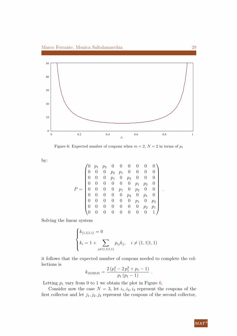
Figure 6: Expected number of coupons when m = 2, N = 2 in terms of p1
by:
P =
0 p1 p2 0 0 0 0 0 00 0 0 p2 p1 0 0 0 00 0 0 p1 0 p2 0 0 00 0 0 0 0 0 p1 p2 00 0 0 0 p1 0 p2 0 00 0 0 0 0 p2 0 p1 00 0 0 0 0 0 p1 0 p20 0 0 0 0 0 0 p2 p10 0 0 0 0 0 0 0 1
.
Solving the linear systemk(1,1|1,1) = 0
ki = 1 +∑
j 6=(1,1|1,1)
pijkj, i 6= (1, 1|1, 1)
it follows that the expected number of coupons needed to complete the col-lections is
k(0,0|0,0) =2 (p41 − 2 p31 + p1 − 1)
p1 (p1 − 1).
Letting p1 vary from 0 to 1 we obtain the plot in Figure 6.Consider now the case N = 3, let i1, i2, i3 represent the coupons of the
first collector and let j1, j2, j3 represent the coupons of the second collector,
MAT 2MATerials MATematicsVolum 2006, treball no. 1, 14 pp.Publicacio electronica de divulgacio del Departament de Matematiquesde la Universitat Autonoma de Barcelonawww.mat.uab.cat/matmat
Trigonometria esferica i hiperbolicaJoan Girbau
L’objectiu d’aquestes notes es establir de forma curta i elegant les formulesfonamentals de la trigonometria esferica i de la trigonometria hiperbolica.La redaccio consta, doncs, de dues seccions independents, una dedicada a latrigonometria esferica i l’altra, a la hiperbolica. La primera esta adrecada aestudiants de primer curs de qualsevol carrera tecnica. La segona requereixdel lector coneixements rudimentaris de varietats de Riemann.
1 Trigonometria esferica
Aquells lectors que ja sapiguen que es un triangle esferic i com es mesuren elsseus costats i els seus angles poden saltar-se les subseccions 1.1 i 1.2 i passardirectament a la subseccio 1.3.
1.1 Arc de circumferencia determinat per dos punts
A cada dos punts A i B de la circumferencia unitat, no diametralment opo-sats, els hi associarem un unic arc de circumferencia, de longitud menor que!, (vegeu la figura 1) tal com explicarem a continuacio.
A
B
O
figura 1
30 The Coupon Collector’s Problem
hence the general state of the Markov Chain will be (i1, i2, i3|j1, j2, j3), andthe state space is given by:
S = {(0, 0, 0|0, 0, 0), (1, 0, 0|0, 0, 0), (0, 1, 0|0, 0, 0), (0, 0, 1|0, 0, 0),
(1, 0, 0|1, 0, 0), (1, 1, 0|0, 0, 0), (1, 0, 1|0, 0, 0), (0, 1, 0|0, 1, 0),
(0, 1, 1|0, 0, 0), (0, 0, 1|0, 0, 1), (1, 1, 0|1, 0, 0), (1, 0, 1|1, 0, 0),
(1, 1, 0|0, 1, 0), (1, 1, 1|0, 0, 0), (1, 0, 1|0, 0, 1), (0, 1, 1|0, 1, 0),
(0, 1, 1|0, 0, 1), (1, 1, 0|1, 1, 0), (1, 1, 1|1, 0, 0), (1, 0, 1|1, 0, 1),
(1, 1, 1|0, 1, 0), (1, 1, 1|0, 0, 1), (0, 1, 1|0, 1, 1), (1, 1, 1|1, 1, 0),
(1, 1, 1|1, 0, 1), (1, 1, 1|0, 1, 1), (1, 1, 1|1, 1, 1)} .
Let p1 be the probability of getting a coupon of type 1, let p2 be the proba-bility of getting a coupon of type 2 and let p3 = 1−p1−p2 be the probabilityof getting a coupon of type 3; the transition matrix has order 27 and solvingthe linear system
k(1,1,1|1,1,1) = 0
ki = 1 +∑
j 6=(1,1,1|1,1,1)
pijkj, i 6= (1, 1, 1|1, 1, 1)
we get the expected waiting time to complete the collections:
k(0,0,0|0,0,0) = 2
[1− 1
1− p1+
1
p1− 1
1− p2+
1
p2+
1
1− p1 − p2
+8 p31 p2 (1− p1 − p2)
(1− p1)3− 3 p41 p2 (1− p1 − p2)
(1− p1)3− 1
p1 + p2
+ p21
(−1 +
1
(1− p2)3− 6 p2 (1− p1 − p2)
(1− p1)3+
1
(p1 + p2)3
)+p1
(1− 1
(1− p2)2− 1
(p1 + p2)2
)].
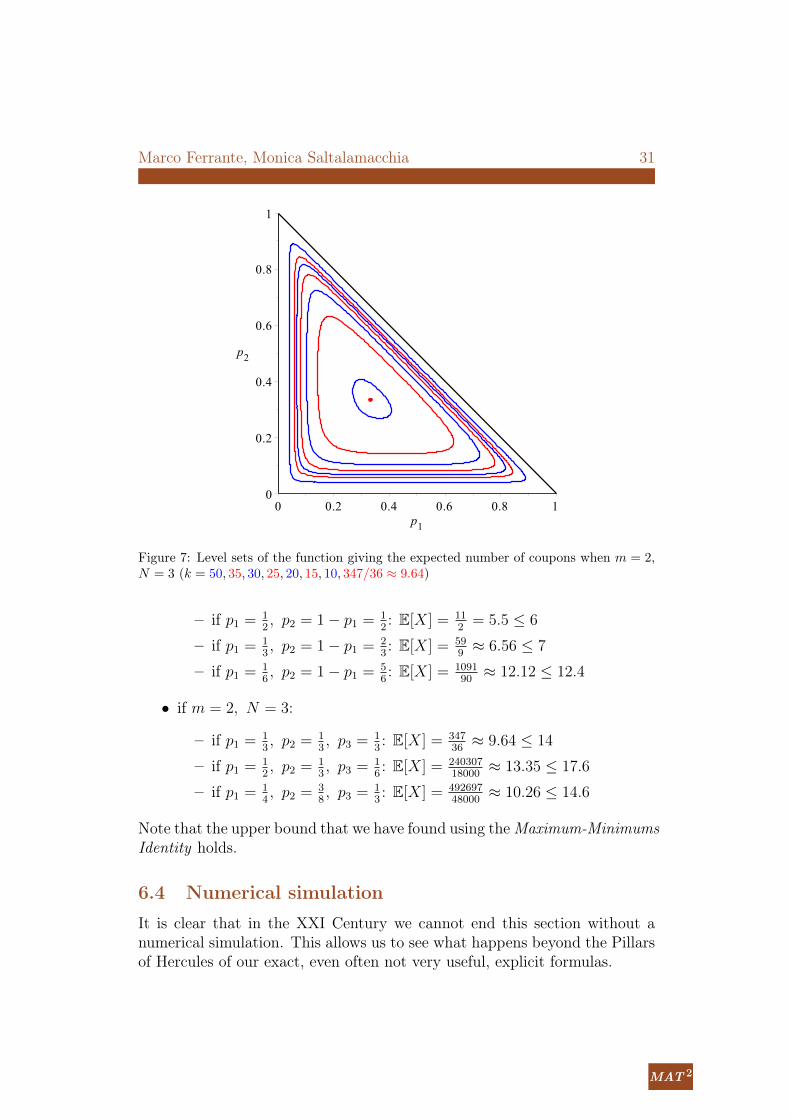
Letting p1 vary from 0 to 1 and p2 from 0 to 1−p1 (to satisfy the constraintp1 + p2 ≤ 1) we obtain the plot of the level sets of the above function inFigure 7; the minimum of this surface corresponds to the point (p1, p2) =(13, 13).
6.3 Examples
• if m = 2, N = 2:
Marco Ferrante, Monica Saltalamacchia 31
Figure 7: Level sets of the function giving the expected number of coupons when m = 2,N = 3 (k = 50, 35, 30, 25, 20, 15, 10, 347/36 ≈ 9.64)
– if p1 = 12, p2 = 1− p1 = 1
2: E[X] = 11
2= 5.5 ≤ 6
– if p1 = 13, p2 = 1− p1 = 2
3: E[X] = 59
9≈ 6.56 ≤ 7
– if p1 = 16, p2 = 1− p1 = 5
6: E[X] = 1091
90≈ 12.12 ≤ 12.4
• if m = 2, N = 3:
– if p1 = 13, p2 = 1
3, p3 = 1
3: E[X] = 347
36≈ 9.64 ≤ 14
– if p1 = 12, p2 = 1
3, p3 = 1
6: E[X] = 240307
18000≈ 13.35 ≤ 17.6
– if p1 = 14, p2 = 3
8, p3 = 1
3: E[X] = 492697
48000≈ 10.26 ≤ 14.6
Note that the upper bound that we have found using theMaximum-MinimumsIdentity holds.
6.4 Numerical simulation
It is clear that in the XXI Century we cannot end this section without anumerical simulation. This allows us to see what happens beyond the Pillarsof Hercules of our exact, even often not very useful, explicit formulas.
MAT 2MATerials MATematicsVolum 2006, treball no. 1, 14 pp.Publicacio electronica de divulgacio del Departament de Matematiquesde la Universitat Autonoma de Barcelonawww.mat.uab.cat/matmat
Trigonometria esferica i hiperbolicaJoan Girbau
L’objectiu d’aquestes notes es establir de forma curta i elegant les formulesfonamentals de la trigonometria esferica i de la trigonometria hiperbolica.La redaccio consta, doncs, de dues seccions independents, una dedicada a latrigonometria esferica i l’altra, a la hiperbolica. La primera esta adrecada aestudiants de primer curs de qualsevol carrera tecnica. La segona requereixdel lector coneixements rudimentaris de varietats de Riemann.
1 Trigonometria esferica
Aquells lectors que ja sapiguen que es un triangle esferic i com es mesuren elsseus costats i els seus angles poden saltar-se les subseccions 1.1 i 1.2 i passardirectament a la subseccio 1.3.
1.1 Arc de circumferencia determinat per dos punts
A cada dos punts A i B de la circumferencia unitat, no diametralment opo-sats, els hi associarem un unic arc de circumferencia, de longitud menor que!, (vegeu la figura 1) tal com explicarem a continuacio.
A
B
O
figura 1
32 The Coupon Collector’s Problem
0 5 10 15 20 25 30 35 40 45 500
500
1000
1500
2000
2500Uniform distribution
N
mea
n
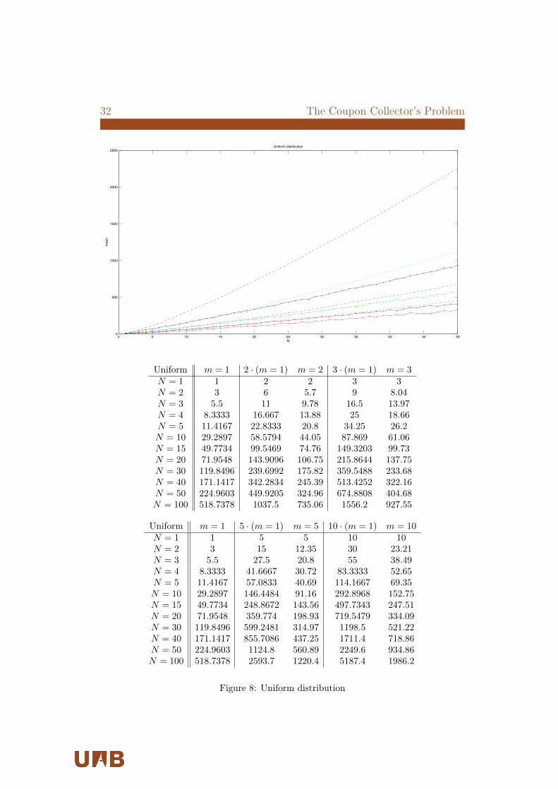
Uniform m = 1 2 · (m = 1) m = 2 3 · (m = 1) m = 3N = 1 1 2 2 3 3N = 2 3 6 5.7 9 8.04N = 3 5.5 11 9.78 16.5 13.97N = 4 8.3333 16.667 13.88 25 18.66N = 5 11.4167 22.8333 20.8 34.25 26.2N = 10 29.2897 58.5794 44.05 87.869 61.06N = 15 49.7734 99.5469 74.76 149.3203 99.73N = 20 71.9548 143.9096 106.75 215.8644 137.75N = 30 119.8496 239.6992 175.82 359.5488 233.68N = 40 171.1417 342.2834 245.39 513.4252 322.16N = 50 224.9603 449.9205 324.96 674.8808 404.68N = 100 518.7378 1037.5 735.06 1556.2 927.55
Uniform m = 1 5 · (m = 1) m = 5 10 · (m = 1) m = 10N = 1 1 5 5 10 10N = 2 3 15 12.35 30 23.21N = 3 5.5 27.5 20.8 55 38.49N = 4 8.3333 41.6667 30.72 83.3333 52.65N = 5 11.4167 57.0833 40.69 114.1667 69.35N = 10 29.2897 146.4484 91.16 292.8968 152.75N = 15 49.7734 248.8672 143.56 497.7343 247.51N = 20 71.9548 359.774 198.93 719.5479 334.09N = 30 119.8496 599.2481 314.97 1198.5 521.22N = 40 171.1417 855.7086 437.25 1711.4 718.86N = 50 224.9603 1124.8 560.89 2249.6 934.86N = 100 518.7378 2593.7 1220.4 5187.4 1986.2
Figure 8: Uniform distribution
Marco Ferrante, Monica Saltalamacchia 33
0 5 10 15 20 25 30 35 40 45 500
0.5
1
1.5
2
2.5
3
3.5
4x 10⁴ Mandelbrot distribution
N
mea
n
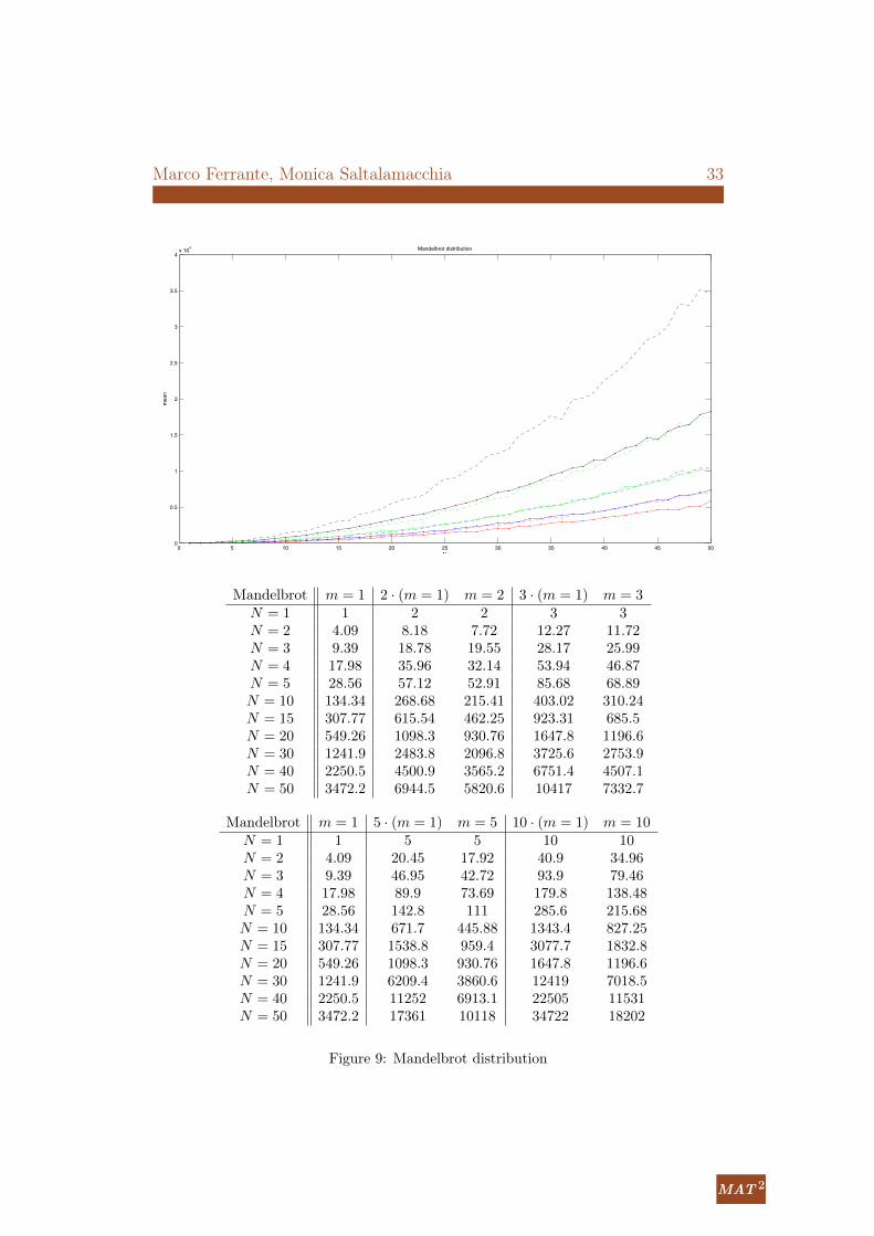
Mandelbrot m = 1 2 · (m = 1) m = 2 3 · (m = 1) m = 3N = 1 1 2 2 3 3N = 2 4.09 8.18 7.72 12.27 11.72N = 3 9.39 18.78 19.55 28.17 25.99N = 4 17.98 35.96 32.14 53.94 46.87N = 5 28.56 57.12 52.91 85.68 68.89N = 10 134.34 268.68 215.41 403.02 310.24N = 15 307.77 615.54 462.25 923.31 685.5N = 20 549.26 1098.3 930.76 1647.8 1196.6N = 30 1241.9 2483.8 2096.8 3725.6 2753.9N = 40 2250.5 4500.9 3565.2 6751.4 4507.1N = 50 3472.2 6944.5 5820.6 10417 7332.7
Mandelbrot m = 1 5 · (m = 1) m = 5 10 · (m = 1) m = 10N = 1 1 5 5 10 10N = 2 4.09 20.45 17.92 40.9 34.96N = 3 9.39 46.95 42.72 93.9 79.46N = 4 17.98 89.9 73.69 179.8 138.48N = 5 28.56 142.8 111 285.6 215.68N = 10 134.34 671.7 445.88 1343.4 827.25N = 15 307.77 1538.8 959.4 3077.7 1832.8N = 20 549.26 1098.3 930.76 1647.8 1196.6N = 30 1241.9 6209.4 3860.6 12419 7018.5N = 40 2250.5 11252 6913.1 22505 11531N = 50 3472.2 17361 10118 34722 18202
Figure 9: Mandelbrot distribution
MAT 2MATerials MATematicsVolum 2006, treball no. 1, 14 pp.Publicacio electronica de divulgacio del Departament de Matematiquesde la Universitat Autonoma de Barcelonawww.mat.uab.cat/matmat
Trigonometria esferica i hiperbolicaJoan Girbau
L’objectiu d’aquestes notes es establir de forma curta i elegant les formulesfonamentals de la trigonometria esferica i de la trigonometria hiperbolica.La redaccio consta, doncs, de dues seccions independents, una dedicada a latrigonometria esferica i l’altra, a la hiperbolica. La primera esta adrecada aestudiants de primer curs de qualsevol carrera tecnica. La segona requereixdel lector coneixements rudimentaris de varietats de Riemann.
1 Trigonometria esferica
Aquells lectors que ja sapiguen que es un triangle esferic i com es mesuren elsseus costats i els seus angles poden saltar-se les subseccions 1.1 i 1.2 i passardirectament a la subseccio 1.3.
1.1 Arc de circumferencia determinat per dos punts
A cada dos punts A i B de la circumferencia unitat, no diametralment opo-sats, els hi associarem un unic arc de circumferencia, de longitud menor que!, (vegeu la figura 1) tal com explicarem a continuacio.
A
B
O
figura 1
34 The Coupon Collector’s Problem
In figures 8 and 9 we have considered the present case with several coop-erative collectors and an arbitrary number of coupons that arrives accordingto the uniform probability distribution or to a Mandelbrot distribution withparameters c = 0.30 and θ = 1.75. To see how big will be in this casethe expected number of coupons to be collected in order to complete all thecollections, we have simulated a big number of virtual collections. Then wehave evaluated the arithmetic mean of the number of coupons needed in thesesimulated collections to complete the sets.
We also have plotted the numerical simulated values (solid line) and com-pared them withm times the expected number of coupons needed to completea single collection (dashed line), again trough a simulation, to see how muchmoney we save in the case of a cooperative collection; in particular, we haveplotted in red the case m = 2, in blue the case m = 3, in green the casem = 5 and in black the case m = 10.
From these computations we observe that if N = 50, in the case of theuniform distribution we can save about the 27% of our money in the case ofm = 2 and that this increases up to a 58% when m = 10, while in the caseof the Mandelbrot distribution we can save about the 16% of our money inthe case of m = 2 and about the 47% when m = 10.
References[1] M. Ferrante, N. Frigo, A note on the coupon-collector’s problem with
multiple arrivals and the random sampling, arXiv:1209.2667v2, 2012.
[2] M. Ferrante, N. Frigo, On the expected number of different records in arandom sample, arXiv:1209.4592v1, 2012.
[3] P. Flajolet, D. Gardy, L. Thimonier, Birthday paradox, coupon collec-tors, caching algorithms and self-organizing search, Discrete Appl. Math.,39:207-229, 1992.
[4] L. Holst, On birthday, collectors’, occupancy and other classical urn prob-lems, Internat. Statist. Rev., 54:15-27, 1986.
[5] D. van Leijenhorst, Th. van der Weide, A formal derivation of Heaps’Law, Information Sciences, 170: 263-272, 2005.
[6] T. Nakata, Coupon collector’s problem with unlike probabilities, Preprint,2008.
[7] D. J. Newman, L. Shepp, The double dixie cup problem, American Math-ematical Monthly, 67:58-61, 1960.
Marco Ferrante, Monica Saltalamacchia 35
[8] S. Ross, A first course in probability, 9th Edition, Pearson, 2012.
[9] W. Stadje, The collector’s problem with group drawings, Advances in Ap-plied Probability, 22:866-882, 1990.
[10] H. von Schelling, Coupon collecting for unequal probabilities, AmericanMathematical Monthly, 61:306-311, 1954.
Marco FerranteDipartimento di MatematicaUniversità degli Studi di PadovaPadova, [email protected]
Monica SaltalamacchiaDipartimento di MatematicaUniversità degli Studi di PadovaPadova, [email protected]
Publicat el 25 de maig de 2014
MAT 2MATerials MATematicsVolum 2006, treball no. 1, 14 pp.Publicacio electronica de divulgacio del Departament de Matematiquesde la Universitat Autonoma de Barcelonawww.mat.uab.cat/matmat
Trigonometria esferica i hiperbolicaJoan Girbau
L’objectiu d’aquestes notes es establir de forma curta i elegant les formulesfonamentals de la trigonometria esferica i de la trigonometria hiperbolica.La redaccio consta, doncs, de dues seccions independents, una dedicada a latrigonometria esferica i l’altra, a la hiperbolica. La primera esta adrecada aestudiants de primer curs de qualsevol carrera tecnica. La segona requereixdel lector coneixements rudimentaris de varietats de Riemann.
1 Trigonometria esferica
Aquells lectors que ja sapiguen que es un triangle esferic i com es mesuren elsseus costats i els seus angles poden saltar-se les subseccions 1.1 i 1.2 i passardirectament a la subseccio 1.3.
1.1 Arc de circumferencia determinat per dos punts
A cada dos punts A i B de la circumferencia unitat, no diametralment opo-sats, els hi associarem un unic arc de circumferencia, de longitud menor que!, (vegeu la figura 1) tal com explicarem a continuacio.
A
B
O
figura 1