TREBALL DE FI DE CARRERA - upcommons.upc.edu · aerodinámica de los vehículos de transporte de...
121
TREBALL DE FI DE CARRERA TÍTOL DEL TFC: Numerical study on Aerodynamic Drag reduction of Passenger Cars TITULACIÓ: Enginyeria Tècnica Aeronàutica, especialitat Aeronavegació AUTORS: Javier Sánchez Martínez DIRECTOR: Fernando Mellibovsky Elstein DATA: 30 de Setembre de 2015
Transcript of TREBALL DE FI DE CARRERA - upcommons.upc.edu · aerodinámica de los vehículos de transporte de...
TREBALL DE FI DE CARRERA
TÍTOL DEL TFC: Numerical study on Aerodynamic Drag reduction of Passenger Cars TITULACIÓ: Enginyeria Tècnica Aeronàutica, especialitat Aeronavegació AUTORS: Javier Sánchez Martínez DIRECTOR: Fernando Mellibovsky Elstein DATA: 30 de Setembre de 2015

Título: Numerical study on Aerodynamic Drag reduction of Passenger Cars Autor: Javier Sánchez Martínez Director: Fernando Mellibovsky Elstein Fecha: 30 de Septiembre de 2015 Resumen El alcance de este trabajo es la identificación de potenciales mejoras en la aerodinámica de los vehículos de transporte de pasajeros (reducción de la resistencia al avance) para ayudar a minimizar el consumo de combustible y por lo tanto reducir las emisiones de contaminantes. El Ahmed body (Bluff body) es una geometría representativa del comportamiento de un vehículo de pasajeros bajo el punto de vista aerodinámico. Existen muchos estudios y literatura publicada, así como reports de ensayos en túneles de viento del Ahmed Body. En este Trabajo se han realizado varias series de simulaciones sobre la geometría base del modelo Ahmed Body con diferentes valores del ángulo trasero. El Ahmed Body con un ángulo de 25º ha sido seleccionado como modelo base para este estudio, pero ha sido modificado con diferentes mejoras aerodinámicas tales como la adición de un difusor al final del bajopiso y la implementación de una forma cóncava en los flancos traseros del modelo, estudiando diferentes configuraciones, y siempre con el objetivo de reducir la resistencia al avance pero respetando la arquitectura del vehículo. Palabras clave: Automoción, Aerodinámica, Ahmed Body, CFD, reducción de Drag, Consumo de combustible

Title: Numerical study of Aerodynamic Drag reduction of Passenger Cars Author: Javier Sánchez Martínez Director: Fernando Mellibovsky Elstein Date: September, 30th 2015 Overview The scope of this work is to identify potential improvements on Passenger cars (Aerodynamics Drag reduction) to help to minimize fuel consumption and hence reduce exhaust emissions. The Ahmed body (Bluff body) is representative of a passenger car under aerodynamic point of view. A lot of studies and literature exists as far as test reports of the Ahmed body on wind tunnel tests. On this work several simulation series had been performed on a 3D model of an Ahmed body with different slant angle values. The Ahmed Body with slant angle of 25º has been selected to be the base configuration for this study, but it has been modified with different aerodynamic improvements such as diffuser integration downstream on the underbody and a concave tail boat shape on the rear of the model, studying different configurations and having always in mind the target of Drag reduction but respecting the vehicle architecture. Keywords: Automotive, Aerodynamics, Ahmed Body, CFD, Drag reduction, Fuel consumption
INDEX
INTRODUCTION ................................................................................................ 1
CHAPTER 1. REFERENCE MODELS ............................................................ 3
1.1 Bluff Body ........................................................................................................................... 3
1.2 Ahmed Body ....................................................................................................................... 3
1.3 Common rear designs of passenger cars ....................................................................... 4
1.4 SAE model .......................................................................................................................... 5
1.5 DrivAer Models .................................................................................................................. 5
1.6 Active and Passive Drag reduction methods ................................................................. 9 1.6.1 Active ..................................................................................................................... 9 1.6.2 Passive .................................................................................................................. 9
1.7 Literature review and published works ........................................................................... 9 1.7.1 Flow over the Ahmed Body ................................................................................. 9 1.7.2 Effect of backlight angle on drag ...................................................................... 10 1.7.3 Effect of Reynolds number ................................................................................ 11 1.7.4 Computational investigations on the Ahmed body ........................................ 12 1.7.5 Drag reduction techniques ................................................................................ 13 1.7.6 Aerodynamic shape optimization ..................................................................... 15
CHAPTER 2. LOW SPEED WIND TUNNELS .............................................. 17
2.1 Wind tunnel principles .................................................................................................... 17
2.2 Theory of use ................................................................................................................... 18
2.3 Types ................................................................................................................................ 19 2.3.1 Air circulation inside .......................................................................................... 19 2.3.2 Flow velocity inside ............................................................................................ 21
2.4 Components ..................................................................................................................... 21 2.4.1 Fan ....................................................................................................................... 21 2.4.2 Test Section ........................................................................................................ 21 2.4.3 Stabilizers and Vanes ......................................................................................... 21 2.4.4 Windows .............................................................................................................. 21 2.4.5 Diffuser ................................................................................................................ 22 2.4.6 Contraction cone ................................................................................................ 22
2.5 Measurement problems on a wind tunnel ..................................................................... 22 2.5.1 Scale effect limitations ....................................................................................... 22 2.5.2 Model dimensions .............................................................................................. 22 2.5.3 Interference Problems (blockage effect) .......................................................... 23
2.6 Fundamentals of Fluid Mechanics for Low speed Wind Tunnels .............................. 23 2.6.1 Boundary Layer .................................................................................................. 23 2.6.2 The Continuity Equation .................................................................................... 24 2.6.3 Bernouilli Equation ............................................................................................. 25

CHAPTER 3. THEORY ................................................................................. 27
3.1 Vehicle aerodynamics ..................................................................................................... 27 3.1.1 Drag ...................................................................................................................... 28 3.1.2 Lift ........................................................................................................................ 30 3.1.3 Ground effect ...................................................................................................... 31
3.2 Motor vehicle dynamics .................................................................................................. 31 3.2.1 Total Resistance Force ...................................................................................... 31 3.2.2 Power ................................................................................................................... 32
3.3 CFD ................................................................................................................................... 34 3.3.1 Fluid Dynamics ................................................................................................... 34 3.3.2 Governing equations .......................................................................................... 35 3.3.3 RANS .................................................................................................................... 37 3.3.4 Turbulence flow and turbulence modeling ...................................................... 37 3.3.5 Boundary Layers and Wall Functions .............................................................. 38
CHAPTER 4. CAD MODELLING AND CFD SIMULATIONS ....................... 41
4.1 CAD ................................................................................................................................... 41 4.1.1 Solid mechanical properties.............................................................................. 42
4.2 CFD Design Modeler and Meshing process ................................................................. 43
4.3 CFD Setup and Boundary Conditions ........................................................................... 56 4.3.1 Set up for 100 iterations ..................................................................................... 57 4.3.2 Set up until convergence ................................................................................... 63 4.3.3 Pressure inlet additional set up ........................................................................ 65
4.4 Solutions .......................................................................................................................... 67
CHAPTER 5. STUDY OF DRAG REDUCTION ............................................ 69
5.1 Ahmed Body ..................................................................................................................... 69 5.1.1 Ahmed Body Wind tunnel vs. CFD: Drag coefficient ...................................... 69 5.1.1 Ahmed Body 25º slant CFD: Pressure coefficient study ................................ 72 5.1.2 Turbulent Intensity and trailing vortex cores .................................................. 76
5.2 Ahmed Body 25º slant + Diffuser ................................................................................... 80 5.2.1 Pressure coefficient study ................................................................................. 81 5.2.2 Turbulent Intensity and trailing vortex cores .................................................. 81
5.3 Ahmed Body 25º slant + 6º Diffuser + Radius .............................................................. 85 5.3.1 Pressure coefficient study ................................................................................. 85 5.3.2 Turbulent Intensity and trailing vortex cores .................................................. 86
5.4 Ahmed Body 25º slant + 6º Diffuser + R 35 + Tail boat ................................................ 90 5.4.1 Pressure coefficient study ................................................................................. 90 5.4.2 Turbulent Intensity and Trailing vortex cores ................................................. 90
5.5 Comparison of the Ahmed Body 25º slant and the Ahmed Body 25º slant + 6º Diffuser + R 35 + 10º Tail boat .................................................................................................. 94
5.6 Simulations with Pressure inlet ..................................................................................... 95 5.6.1 Low position........................................................................................................ 96 5.6.2 High position ....................................................................................................... 96

CHAPTER 6. CONCLUSIONS ...................................................................... 97
6.1 Aerodynamic analysis conclusions .............................................................................. 97
6.2 General Conclusions ....................................................................................................... 98 6.2.1 Power required and Fuel consumption ............................................................ 98 6.2.2 Emissions .......................................................................................................... 100
6.3 Further job ...................................................................................................................... 101
BIBLIOGRAPHY ............................................................................................ 103
LIST OF FIGURES
Figure 1 – Schematic of Ahmed body (Ahmed, 1984) (a) Dimensions, (b) Slant angle configurations .................................................................................... 4
Figure 2 – Common generic rear body designs (a) Notchback (b) Fastback and (c) Squareback ............................................................................................ 5
Figure 3 – 3D SAE body ..................................................................................... 5
Figure 4 – Main dimensions of the DrivAer Fast back model Scale (1:2.5) ........ 6
Figure 5 – DrivAer body with different back shape ............................................. 7
Figure 6 – Underbody configurations: (a) detailed (b) smooth............................ 7
Figure 7 – Schematic diagram of flow in the wake of Ahmed Body .................. 11
Figure 8 – Variation of Cd of the Ahmed Body with base slant angle (α) ......... 12
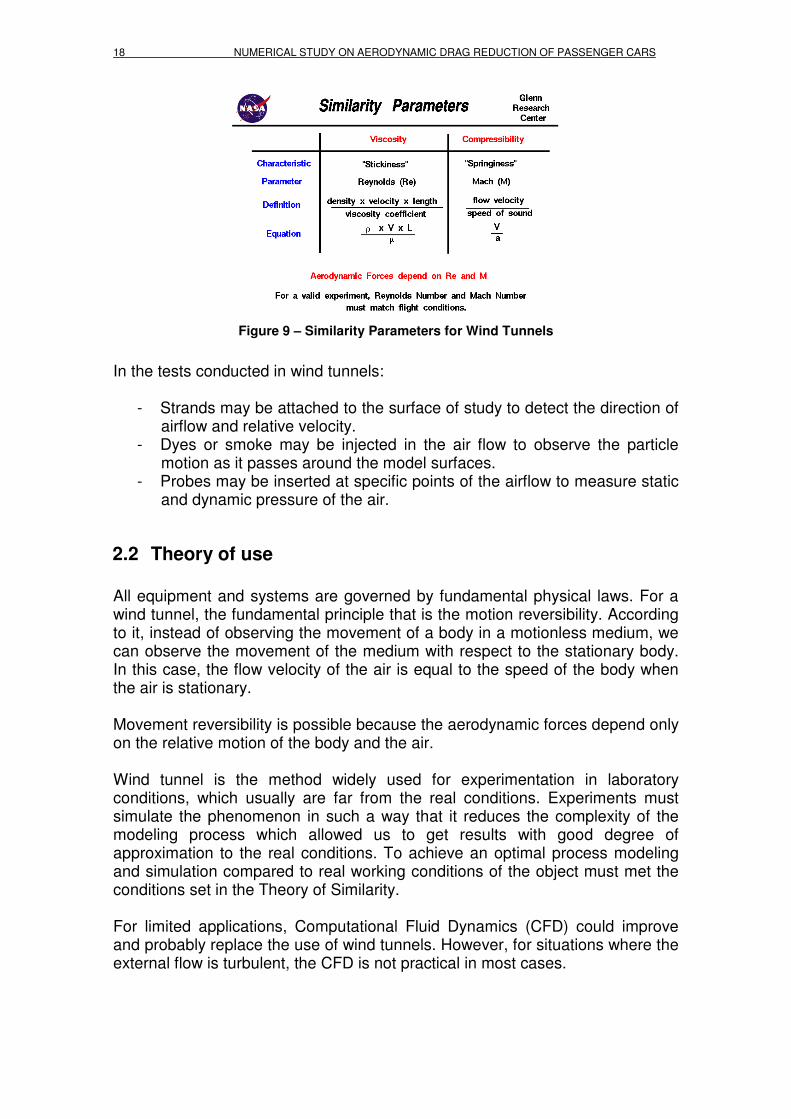
Figure 9 – Similarity Parameters for Wind Tunnels .......................................... 18
Figure 10 – Open wind tunnel .......................................................................... 19
Figure 11 – Closed wind tunnel ........................................................................ 20
Figure 12 – Classification of wind tunnels ........................................................ 21
Figure 13 – Boundary Layer representation (a) Laminar flow (b) turbulent flow 24
Figure 14 – Pressure and shear over a surface ............................................... 27
Figure 15 – Decomposition of R in 2 components ............................................ 27
Figure 16 – Aerodynamic Forces acting on a car ............................................. 28
Figure 17 – Cd of different body shapes .......................................................... 29
Figure 18 – Specific energy consumption (for medium size passenger cars) [25] .................................................................................................................. 33
Figure 19 – Velocity profile in the boundary layer on a flat plate (Cartesian) ... 39
Figure 20 – Velocity profile in the near wall region (logaritmic) ........................ 39
Figure 21 – Ahmed Body dimensions [3] .......................................................... 41
Figure 22 – Ahmed Body dimensions 25º slant ................................................ 42
Figure 23 – Solid mechanical properties of the Ahmed 25º .............................. 43
Figure 24 – Control Volume dimensions (Side View) ....................................... 44
Figure 25 – Control Volume dimensions (Front view) ....................................... 44
Figure 26 – CFD element types ........................................................................ 45
Figure 27 – First coarse mesh parameters ....................................................... 45
Figure 28 – First coarse mesh .......................................................................... 45
Figure 29 – Zoom of the first coarse mesh ....................................................... 46
Figure 30 – Skewness of the first coarse mesh attempt ................................... 46
Figure 31 – First sizing applied on the stilt surfaces ......................................... 46
Figure 32 – Second sizing function applied to the Ahmed body surfaces ........ 47
Figure 33 – Mesh after surface sizing functions application ............................. 47
Figure 34 – Zoom of the mesh after surface sizing functions application ......... 47
Figure 35 – Skewness of the mesh without refinements .................................. 47
Figure 36 – Ahmed Body projected area .......................................................... 48
Figure 37 – Named Selections ......................................................................... 49
Figure 38 – Ahmed body selection ................................................................... 49
Figure 39 – Symmetry selection ....................................................................... 50
Figure 40 – Velocity-inlet selection ................................................................... 50
Figure 41 – Symmetry top selection ................................................................. 50
Figure 42 – Pressure-outlet selection ............................................................... 50
Figure 43 – Ground selection ........................................................................... 51
Figure 44 – Symmetry-side selection ............................................................... 51
Figure 45 – Inflation parameters ....................................................................... 51
Figure 46 – Mesh after inflation ........................................................................ 51
Figure 47 – Zoom of the mesh after inflation .................................................... 52
Figure 48 – Skewness of the mesh after inflation ............................................. 52
Figure 49 – Carbox ........................................................................................... 53
Figure 50 – Carbox sizing function parameters ................................................ 53
Figure 51 – Carbox influence on the mesh ....................................................... 53
Figure 52 – Zoom of the carbox influence on the mesh ................................... 53
Figure 53 – Skewness after application of the carbox control volume .............. 54
Figure 54 – Underbody ..................................................................................... 54
Figure 55 – Underbody sizing function parameters .......................................... 54
Figure 56 – Underbody influence on the mesh ................................................. 54
Figure 57 – Skewness after application of the underbody control volume ........ 55
Figure 58 – Wakebox box................................................................................. 55
Figure 59 – Wakebox box sizing function parameters ...................................... 55
Figure 60 – Wakebox box influence on the mesh ............................................. 55
Figure 61 – Skewness after application of the underbody box control volume . 56
Figure 62 – Mesh check ................................................................................... 56
Figure 63 – Case .............................................................................................. 57
Figure 64 – Viscous model ............................................................................... 58
Figure 65 – Velocity inlet .................................................................................. 58
Figure 66 – Pressure outlet .............................................................................. 59
Figure 67 – Reference values .......................................................................... 59
Figure 68 – Solution methods ........................................................................... 60
Figure 69 – Solution controls ............................................................................ 60
Figure 70 – Solution limits ................................................................................ 61
Figure 71 – Residual monitors .......................................................................... 61
Figure 72 – Drag monitor ................................................................................. 61
Figure 73 – Lift monitor .................................................................................... 62
Figure 74 – Moment monitor ............................................................................ 62
Figure 75 – Hybrid initialization ........................................................................ 63
Figure 76 – Calculation: 100 iterations ............................................................. 63
Figure 77 – Solution methods ........................................................................... 63
Figure 78 – Solution controls ............................................................................ 64
Figure 79 – Run calculation .............................................................................. 64
Figure 80 – Residuals plot ................................................................................ 64
Figure 81 – Drag coefficient plot ....................................................................... 65
Figure 82 – Lift coefficient plot .......................................................................... 65
Figure 83 – Moment plot .................................................................................. 65
Figure 84 – Pressure inlet ................................................................................ 66
Figure 85 – Drag breakdown for three configurations (Ahmed 1984) [3] .......... 69
Figure 86 – Variation of Cd of the Ahmed Body with base slant angle (α) ....... 70
Figure 87 – Velocity streamlines for Ahmed body 25º slant ............................. 71
Figure 88 – Velocity streamlines for Ahmed body 35º slant ............................. 71
Figure 89 – Relative Pressure Drag contributions (Ahmed 1984) [3] ............... 72
Figure 90 – Contours of Pressure coefficient on the Ahmed body 25º surfaces (a) front, (b) rear ........................................................................................ 73
Figure 91 – Pressure coefficient XY Plot on the symmetry plane of the Ahmed body 25º slant............................................................................................ 73
Figure 92 – Pressure coefficient XY Plot on the symmetry plane of the Ahmed body 30º slant............................................................................................ 74
Figure 93 – Pressure coefficient XY Plot on the symmetry plane of the Ahmed body 35º slant............................................................................................ 74
Figure 94 – Plot of Ahmed 25º flow reattachment on the 25º slant [27] ............ 75
Figure 95 – CFD Ahmed 25º with no flow reattachment on the slant (a) Velocity vectors, (b) Velocity streamlines ............................................................... 76
Figure 96 – Plot of the vectors of Turbulent Intensity on X= -222 plane .......... 76
Figure 97 – Plot of the vectors of Turbulent Intensity on X= -100 plane ........... 77
Figure 98 – Plot of the vectors of Turbulent Intensity on X=0 plane ................. 77
Figure 99 – Plot of the vectors of Turbulent Intensity on X=100 plane ............. 77
Figure 100 – Plot of the vectors of Turbulent Intensity on X= 200 plane .......... 78
Figure 101 – Plot of the vectors of Turbulent Intensity on X= 500 plane .......... 78
Figure 102 – Plot of the vectors of Turbulent Intensity on X= 750 plane .......... 78
Figure 103 – Plot of the vectors of Turbulent Intensity on X= 1000 plane ........ 79
Figure 104 – Plot of the vectors of Turbulent Intensity on X= 1250 plane ........ 79
Figure 105 – Plot of the vectors of Turbulent Intensity on X= 1500 plane ........ 79
Figure 106 – Derived Lambda-2 criteria for Vortex core evaluation (3D) ......... 80
Figure 107 – Pressure coefficient XY Plot on the symmetry plane of the Ahmed body 25º slant + 6º diffuser ....................................................................... 81
Figure 108 – Plot of the vectors of Turbulent Intensity on X= -222 plane ......... 81
Figure 109 – Plot of the vectors of Turbulent Intensity on X= -100 plane ......... 82
Figure 110 – Plot of the vectors of Turbulent Intensity on X=0 plane ............... 82
Figure 111 – Plot of the vectors of Turbulent Intensity on X=100 plane ........... 82
Figure 112 – Plot of the vectors of Turbulent Intensity on X= 200 plane .......... 83
Figure 113 – Plot of the vectors of Turbulent Intensity on X= 500 plane .......... 83
Figure 114 – Plot of the vectors of Turbulent Intensity on X= 750 plane .......... 83
Figure 115 – Plot of the vectors of Turbulent Intensity on X= 1000 plane ........ 84
Figure 116 – Plot of the vectors of Turbulent Intensity on X= 1250 plane ........ 84
Figure 117 – Plot of the vectors of Turbulent Intensity on X= 1500 plane ........ 84
Figure 118 – Derived Lambda-2 criteria for Vortex core evaluation (3D) ......... 85
Figure 119 – Pressure coefficient XY Plot on the symmetry plane of the Ahmed body 25º slant + 6º diffuser + Radius 35 ................................................... 86
Figure 120 – Plot of the vectors of Turbulent Intensity on X= -222 plane ......... 86
Figure 121 – Plot of the vectors of Turbulent Intensity on X= -100 plane ......... 86
Figure 122 – Plot of the vectors of Turbulent Intensity on X=0 plane ............... 87
Figure 123 – Plot of the vectors of Turbulent Intensity on X=100 plane ........... 87
Figure 124 – Plot of the vectors of Turbulent Intensity on X= 200 plane .......... 87
Figure 125 – Plot of the vectors of Turbulent Intensity on X= 500 plane .......... 88
Figure 126 – Plot of the vectors of Turbulent Intensity on X= 750 plane .......... 88
Figure 127 – Plot of the vectors of Turbulent Intensity on X= 1000 plane ........ 88
Figure 128 – Plot of the vectors of Turbulent Intensity on X= 1250 plane ........ 89
Figure 129 – Plot of the vectors of Turbulent Intensity on X= 1500 plane ........ 89
Figure 130 – Derived Lambda-2 criteria for Vortex core evaluation (3D) ......... 89
Figure 131 – Pressure coefficient XY Plot on the symmetry plane of the Ahmed body 25º slant + 6º diffuser + Radius 35 + 10º Tail Boat ........................... 90
Figure 132 – Plot of the vectors of Turbulent Intensity on X= -222 plane ......... 90
Figure 133 – Plot of the vectors of Turbulent Intensity on X= -100 plane ......... 91
Figure 134 – Plot of the vectors of Turbulent Intensity on X=0 plane ............... 91
Figure 135 – Plot of the vectors of Turbulent Intensity on X=100 plane ........... 91
Figure 136 – Plot of the vectors of Turbulent Intensity on X= 200 plane .......... 92
Figure 137 – Plot of the vectors of Turbulent Intensity on X= 500 plane .......... 92
Figure 138 – Plot of the vectors of Turbulent Intensity on X= 750 plane .......... 92
Figure 139 – Plot of the vectors of Turbulent Intensity on X= 1000 plane ........ 93
Figure 140 – Plot of the vectors of Turbulent Intensity on X= 1250 plane ........ 93
Figure 141 – Plot of the vectors of Turbulent Intensity on X= 1500 plane ........ 93
Figure 142 – Derived Landa-2 criteria for Vortex core evaluation (3D) ............ 94
Figure 143 – Pressure coefficients comparison (a) Ahmed 25º slant, (b) Ahmed 25º slant + 6º diffuser + R35 + 10º Boat tail .............................................. 95
Figure 144 – Pressure inlet surface, low position ............................................. 96
Figure 145 – Pressure inlet surface, high position ............................................ 96
Figure 146 - Example energy flows for a late-model midsize passenger car: (a) urban driving; (b) highway driving. [26] ................................................... 100

LIST OF TABLES
Table 1 – Comparison of the CD DrivAer, Audi A4 and BMW 3 Series .............. 8
Table 2 – Cd of DrivAer Notchback, Fastback and Estateback configurations ... 8
Table 3 – Basic criteria for automotive aerodynamic design [4] ....................... 14
Table 4 – Models configuration ........................................................................ 42
Table 5 – First design iteration Cd results and error calculation ....................... 70
Table 6 – Comparison of Experimental and Simulation Cd values ................... 70
Table 7 – Second design iteration Cd results ................................................... 81
Table 8 – Third design iteration Cd results ....................................................... 85
Table 9 – Fourth design iteration Cd results ..................................................... 90
Table 10 – Fifth design iteration Cd results ...................................................... 96
Table 11 – Contribution to Cd reduction ........................................................... 97
Table 12 – Fuel consumption calculation table ................................................ 99


ACCRONYMS, ABBREVIATIONS AND DEFINITIONS ANSYS Analysis System CAD Computer Aided Design CATIA Computer Aided Three-dimensional Interactive Application CFD Computational Fluid Dynamics CG Center of Gravity DES Detached Eddy Simulations LES Large Eddy Simulations RANS Reynolds Averaged Navier-Stokes

INTRODUCTION 1
INTRODUCTION In recent years, the improvement in fuel efficiency has become a major factor in passenger cars development due to increasing population, global decline in fossil fuel reserves, rising fuel prices and the damaging effects of global warming. The aerodynamic drag of a road vehicle is responsible for a large part of the vehicle’s fuel consumption and it can contribute to as much as 50-75% of the total vehicle fuel consumption at highway speeds [1]. Reducing the aerodynamic drag offers an inexpensive solution to improve fuel efficiency and therefore shape optimization for low drag has become an essential part of the overall vehicle design process. Although the wind tunnels can provide most accurate data and test conditions close to actual road conditions, the large number of design variables and geometric configurations involved at the conceptual stage of vehicle design make wind tunnel experiments very expensive and time consuming. The availability of high performance computers and relatively accurate turbulence models have led to an increased use of computational fluid dynamics (CFD) software in the development of road vehicles. Shape optimization using CFD also requires numerous computational evaluations for different design configurations and the process can take many days to reach an optimum solution. The time required for CFD simulations and optimization process depends on many factors including the choice of turbulence model, mesh resolution, the number of design parameters, the parameterization process as well as the optimization strategy. In this work, CFD simulations of the flow around the Ahmed body have been done, and the results has been compared with the experimental results [3] to validate the numerical method chosen. Then after, a design and simulation loop has been performed to obtain a final modified Ahmed body that satisfies the objective of this study: Drag reduction. Results analysis has been focused on Coefficient of Drag reduction, Coefficient of Pressure evolution and Turbulence on the wake region of the models. Finally, the benefits of Drag reduction has been quantified in cost savings and pollutant emissions reduction.

CHAPTER 1: REFERENCE MODELS 3
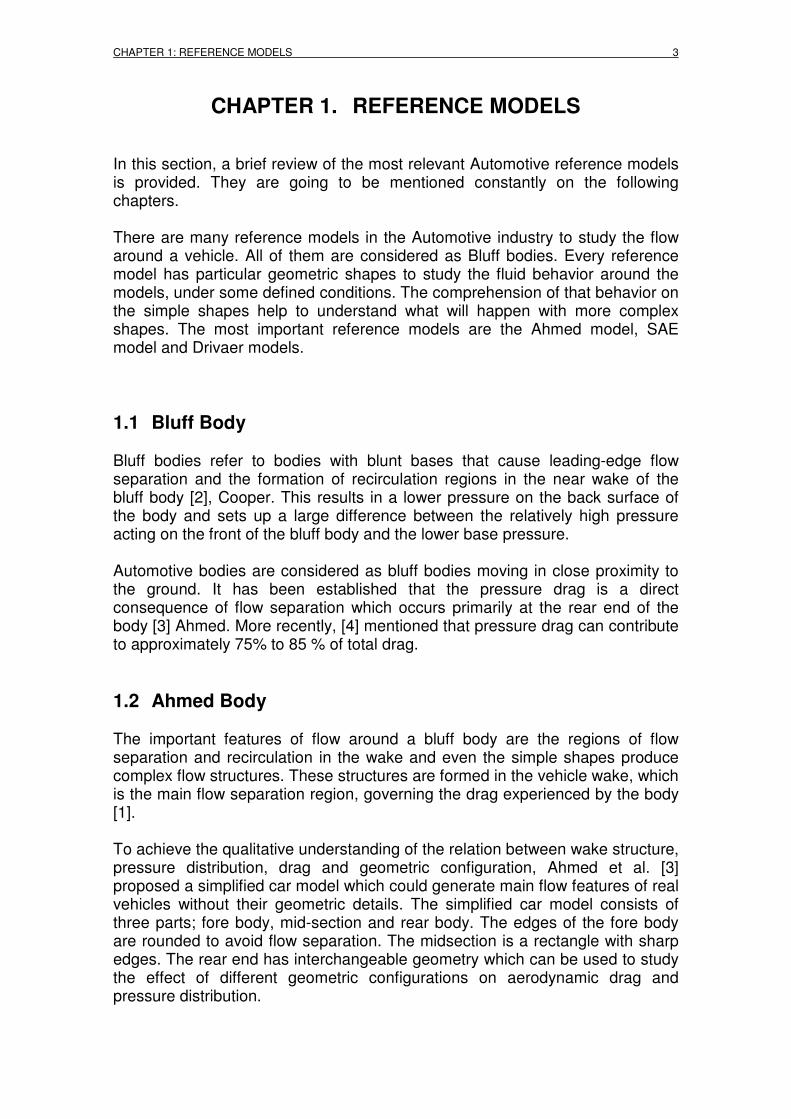
CHAPTER 1. REFERENCE MODELS In this section, a brief review of the most relevant Automotive reference models is provided. They are going to be mentioned constantly on the following chapters. There are many reference models in the Automotive industry to study the flow around a vehicle. All of them are considered as Bluff bodies. Every reference model has particular geometric shapes to study the fluid behavior around the models, under some defined conditions. The comprehension of that behavior on the simple shapes help to understand what will happen with more complex shapes. The most important reference models are the Ahmed model, SAE model and Drivaer models.
1.1 Bluff Body Bluff bodies refer to bodies with blunt bases that cause leading-edge flow separation and the formation of recirculation regions in the near wake of the bluff body [2], Cooper. This results in a lower pressure on the back surface of the body and sets up a large difference between the relatively high pressure acting on the front of the bluff body and the lower base pressure. Automotive bodies are considered as bluff bodies moving in close proximity to the ground. It has been established that the pressure drag is a direct consequence of flow separation which occurs primarily at the rear end of the body [3] Ahmed. More recently, [4] mentioned that pressure drag can contribute to approximately 75% to 85 % of total drag.
1.2 Ahmed Body The important features of flow around a bluff body are the regions of flow separation and recirculation in the wake and even the simple shapes produce complex flow structures. These structures are formed in the vehicle wake, which is the main flow separation region, governing the drag experienced by the body [1]. To achieve the qualitative understanding of the relation between wake structure, pressure distribution, drag and geometric configuration, Ahmed et al. [3] proposed a simplified car model which could generate main flow features of real vehicles without their geometric details. The simplified car model consists of three parts; fore body, mid-section and rear body. The edges of the fore body are rounded to avoid flow separation. The midsection is a rectangle with sharp edges. The rear end has interchangeable geometry which can be used to study the effect of different geometric configurations on aerodynamic drag and pressure distribution.

4 NUMERICAL STUDY ON AERODYNAMIC DRAG REDUCTION OF PASSENGER CARS
In the experiments conducted by Ahmed et al. [3], nine interchangeable rear bodies with different base slants from 0º to 40º were tested. Figure 1 shows the schematic of the original Ahmed body.
(a)
(b)
Figure 1 – Schematic of Ahmed body (Ahmed, 1984) (a) Dimensions, (b) Slant angle configurations
1.3 Common rear designs of passenger cars In passenger car designs, there are three main categories of generic rear geometry: the notch back, the fast back and the square back or station wagon. These generic car bodies and their general wake structure are illustrated in Figure 2. The roof of the notch back drops off at the rear and forms a distinct deck whereas the roof of fast back and square back slopes down continuously at the back. It can also be seen that these generic bodies have distinct wake structures. In the design process, the body stylist selects the type of rear

CHAPTER 1: REFERENCE MODELS 5
geometry based on vehicle function, design and aesthetics and the role of the aerodynamicist is to obtain low drag design based on selected configuration [1].
Figure 2 – Common generic rear body designs (a) Notchback (b) Fastback and (c) Squareback
1.4 SAE model
The SAE model (Figure 3) is used in the automotive industry to study the influence of the flow around vehicle considering the effects of the front of the vehicle as well as the rear wake region.
Figure 3 – 3D SAE body
1.5 DrivAer Models
Generic car models, such as the SAE model and the Ahmed body, make it easy to relate the observed phenomena to specific areas and thus help to understand
6 NUMERICAL STUDY ON AERODYNAMIC DRAG REDUCTION OF PASSENGER CARS
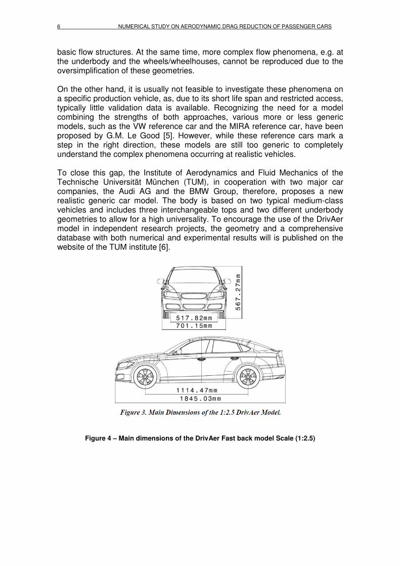
basic flow structures. At the same time, more complex flow phenomena, e.g. at the underbody and the wheels/wheelhouses, cannot be reproduced due to the oversimplification of these geometries. On the other hand, it is usually not feasible to investigate these phenomena on a specific production vehicle, as, due to its short life span and restricted access, typically little validation data is available. Recognizing the need for a model combining the strengths of both approaches, various more or less generic models, such as the VW reference car and the MIRA reference car, have been proposed by G.M. Le Good [5]. However, while these reference cars mark a step in the right direction, these models are still too generic to completely understand the complex phenomena occurring at realistic vehicles. To close this gap, the Institute of Aerodynamics and Fluid Mechanics of the Technische Universität München (TUM), in cooperation with two major car companies, the Audi AG and the BMW Group, therefore, proposes a new realistic generic car model. The body is based on two typical medium-class vehicles and includes three interchangeable tops and two different underbody geometries to allow for a high universality. To encourage the use of the DrivAer model in independent research projects, the geometry and a comprehensive database with both numerical and experimental results will is published on the website of the TUM institute [6].
Figure 4 – Main dimensions of the DrivAer Fast back model Scale (1:2.5)
CHAPTER 1: REFERENCE MODELS 7
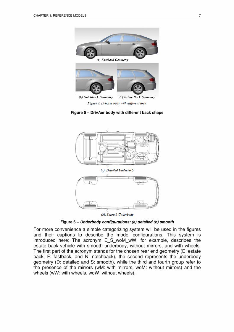
Figure 5 – DrivAer body with different back shape
Figure 6 – Underbody configurations: (a) detailed (b) smooth
For more convenience a simple categorizing system will be used in the figures and their captions to describe the model configurations. This system is introduced here: The acronym E_S_woM_wW, for example, describes the estate back vehicle with smooth underbody, without mirrors, and with wheels. The first part of the acronym stands for the chosen rear end geometry (E: estate back, F: fastback, and N: notchback), the second represents the underbody geometry (D: detailed and S: smooth), while the third and fourth group refer to the presence of the mirrors (wM: with mirrors, woM: without mirrors) and the wheels (wW: with wheels, woW: without wheels).

8 NUMERICAL STUDY ON AERODYNAMIC DRAG REDUCTION OF PASSENGER CARS
Table 1 – Comparison of the CD DrivAer, Audi A4 and BMW 3 Series
Table 2 – Cd of DrivAer Notchback, Fastback and Estateback configurations

CHAPTER 1: REFERENCE MODELS 9
1.6 Active and Passive Drag reduction methods
1.6.1 Active Based upon whether the methods consume energy to control the flow or not, they are classified into active or passive control methods. Active control is performed by using actuators that require a power generally taken on the principal generator of energy of the vehicle. The visible part of these systems includes mobile walls, circular holes or slots distributed on the vehicle surface where the flow must be controlled. Their use requires mechanical, electromagnetic, electric, piezoelectric or acoustic systems placed in the hollow parts of the vehicle. Their weights and their overall dimensions must be smallest as possible to reduce their impacts on consumption and habitable volume. Several control solutions have been identified, tested and analyzed for aeronautics. It has been the same for the hydrodynamic and the aerodynamic of the road vehicles. The adopted solutions generally consist on suction or blowing systems through circular or rectangular slots. The suction and blowing can be continuous or intermittent.
1.6.2 Passive The passive control systems consist on the use of more or less discrete obstacles, added around or on the roof of the vehicle. They can be declined in two groups according to their influence on the flow control. The first group consists on obstacles positioned on the surface of the geometry. The second group consists of the obstacles positioned upstream or downstream of the geometry to be controlled.
1.7 Literature review and published works In this section, a brief review of literature is provided on the following topics: description of flow over Ahmed body, drag reduction techniques and car body aerodynamic shape optimization. The state of the art (January 2014) with regards the Ahmed Body investigations can be found in the paper published by Sudin [7].
1.7.1 Flow over the Ahmed Body In this section, a brief review of literature is provided on the following topics: description of flow over Ahmed body, drag reduction techniques and car body aerodynamic shape optimization. Flow structure around Ahmed body The flow over the Ahmed body remains attached on the front and the mid-section and the boundary layer develops on the surfaces of the model. The boundary layer separation occurs at the rear of the model where the flow from the top, bottom and sides separates and forms shear layers. These shear layers curve towards each other and form a closed region with a stagnation point behind the model. This enclosed region of
10 NUMERICAL STUDY ON AERODYNAMIC DRAG REDUCTION OF PASSENGER CARS
circulating air is called the wake. Although the wake flow of Ahmed body is unsteady, the time averaged flow schematic illustrated in Figure 3 shows important vortex structures that govern the pressure drag produced at the rear end [3]. The experiments conducted by Ahmed et al. [3] investigated the effect of backlight angles in the range of 0º to 40º. The backlight angle is the angle of depression of the rear window. In this range, two critical backlight angles (α) which were identified to have a significant influence on the flow structure were 12.5º and 30º. Three ranges of backlight angles were identified which have different aerodynamic effects: 0º < α < 12.5º; 12.5º < α < 30º ; and α > 30.0º. In the range of 0º < α < 12.5º, the flow remains attached over the rear window slant and separates at the top and bottom edges of the vertical base. The shear layers from the top and bottom roll towards each other and form two circulating regions A and B as depicted in Figure 3a. As the backlight angle increases, the upper circulating region becomes more dominant. The shear layers from the vertical sides of the slanted base roll up and form longitudinal vortices C as shown in Figure 3a. If the flow remains attached on the slanted base, the strength of vortex A and C depends on the backlight angle. In the range of 12.5º < α < 30º, the strength of longitudinal vortex C increases and the flow becomes increasingly three dimensional. These longitudinal vortices are also responsible for maintaining attached flow over the slanted base. Close to 30º backlight angle, a separation bubble D forms on the slanted base but the flow reattaches close to the top edge of the vertical base as shown in Figure 3b. At this point, the flow again separates and forms two circulating regions A and B as described previously. For α greater than 30º, the flow separates at the top edge of the rear window. The two circulating regions A and B are again formed in the wake but the separation bubble D can no longer be distinguished from A, instead, a bigger circulating region is formed which comprises of both A and D.
1.7.2 Effect of backlight angle on drag The trend of drag coefficient over a wide range of backlight angles is shown in Figure 4. The total Cd decreases from 0.250 at 0º to a minimum value of 0.230 at 12.5º. The Cd again increases to a maximum value of 0.378 upon further increase in backlight angle to 30º

CHAPTER 1: REFERENCE MODELS 11
Figure 7 – Schematic diagram of flow in the wake of Ahmed Body
Figure 7 also shows the contributions of different sections of the body to the total drag and it can be inferred that the backlight angle has a significant effect. The relative contribution of drag coefficient (C*s in Figure 7) to the overall pressure drag is most sensitive to the backlight angle. This suggests that the separation bubble on the slanted base causes a higher pressure force on the model. It should be noted that the front geometry has little effect on the pressure drag and does not show any significant relation to the backlight angle. This is because the long middle section does not allow any significant interaction of flow between the front and the rear end. In addition, the value of friction drag also does not exhibit any significant relation to the backlight angle. It is reported that the percentage contribution of friction drag to the total drag remains in the range of 15 to 24% [3].
1.7.3 Effect of Reynolds number The experiments conducted by Ahmed et al. [3] were performed at a wind speed of 60 m/s. This corresponds to a Reynolds number of 4.29 million based on model length. Bayraktar [8] studied the effect of Reynolds number on lift and drag coefficients. The experiments were performed at Reynolds number in the range of 2.2 to 13.2 million. It was observed that over this wide range of Reynolds number, the drag coefficient only altered by 3.5 percent while the lift coefficient altered by 2 percent. Thus it was concluded that the drag coefficient is insensitive at high Reynolds numbers (of the order of 10^6 ).

12 NUMERICAL STUDY ON AERODYNAMIC DRAG REDUCTION OF PASSENGER CARS
Figure 8 – Variation of Cd of the Ahmed Body with base slant angle (α)
1.7.4 Computational investigations on the Ahmed body The Ahmed body lends itself well for CFD studies due to its simple geometry and availability of experimental data. Some difficulties in predicting the overall flow around the Ahmed body using various turbulence models still remains due to the flow separation on the slant rear window and recirculation region in its wake (Krajnovi´c, 2004) [9]. This is partly because the flow in this region is extremely unsteady. Practitioners of CFD strive to develop turbulence models which can predict the real flows as accurately as possible but there is always a compromise between computational cost and accuracy. The availability of high performance computers has enabled the use of highly accurate turbulence models for external flow. Large Eddy Simulation (LES) is a CFD technique where large flow structures are directly computed from Navier Stokes equations and only the structures smaller than the computational cells are modeled (ANSYS FLUENT user’s guide). Since the size of turbulent vortices decreases with increasing Reynolds

CHAPTER 1: REFERENCE MODELS 13
number, LES is performed at moderate Reynolds numbers so that most of the turbulent vortices can be directly solved rather than modelled. Krajnović (2004) [9] performed LES on 25° Ahmed model with 9.6 and 16.5 million cells for medium and fine grids. These studies were performed at low Reynolds number (2×10⁵ ) to facilitate the use of LES. The results of the study were also validated against the data from Lienhart (2003) [10] and concluded that the flow structure around the model was well predicted. In addition, Kapadia (2003) [11] performed Detached Eddy Simulation (DES) with a grid size of 1.74 million cells. This study was performed on 25° and 35° Ahmed bodies. The average drag coefficient from DES for both 25° and 35° angles was within 5% of the experimental value reported by Ahmed (1984) [3]. Kapadia (2003) [11] also performed unsteady simulations using the Re-normalization group (RNG) k-ε turbulence model. The results suggested that the RNG k-ε model over predicts the drag coefficient. It was also mentioned that the cases where the flow is on the verge of separation or at separation and reattachment on rear slant as in 25° case pose a strong challenge to computational methods since small difference in separation prediction can lead to substantial difference between CFD and experimental results. Although the DES and LES have shown superior performance in predicting the overall flow structure, Reynolds averaged Navier Stokes (RANS) equation based turbulence models are chosen for automotive aerodynamics due to limitations of computer RAM and simulation time (Lanfrit, 2005) [12]. Braun (2001) [13] used the Realizable k-ε model for simulation of flow on 25° Ahmed body with 2.3 million grid size. The results suggested that although the RANS models do not predict the actual flow separation on the 25° base slant, the overall results including the drag coefficient are predicted with reasonable accuracy.
1.7.5 Drag reduction techniques Many attempts have been made since the early years in the automotive industry to reduce aerodynamic drag in order to improve performance and fuel economy. Morelli (1976) [4] developed a theoretical method to determine the shape of passenger car body for minimum drag by imposing the condition that the total lift be zero. With this condition and a gradual variation in the area and shape of transverse cross sections of the body, a basic shape was realized with a drag coefficient of 0.23. This study proved that the aerodynamic drag can be reduced substantially with an optimized body shape without any additional devices.

14 NUMERICAL STUDY ON AERODYNAMIC DRAG REDUCTION OF PASSENGER CARS
Later, Morelli (2000) [14] proposed a new technique called “fluid tail” and applied it to the aerodynamic design of basic shape of a passenger car. To achieve a fluid tail, a ring vortex must be created at the rear of the vehicle. A ring vortex is created behind a body when the flow separation line is perpendicular with respect to direction of motion and the flow separation line coincides with or is very close to the body. The perimeter of the body must be circular or elliptical without any deflection and pressure and velocity must be uniform around the perimeter. To achieve these conditions, the rear wheels were fitted with centrifugal fans which directed the flow around the wheels to the rear body through ducts located at the rear bottom. Wind tunnel tests carried on FIAT Punto 55 showed reduction in drag coefficient from 0.327 to 0.268, a drop by 18 %. The basic criteria proposed by Morelli (1976, 2000) [4] [14] are summarized in Table 1. The idea of fluid tail seems quite promising as it is very much similar to “boat tail” which has been studied in great detail and is well understood (Peterson, 1981) [15]. Boat tailing is a technique in which the rear body is tapered which results in pressure recovery at the rear body and reduces pressure drag.
Table 3 – Basic criteria for automotive aerodynamic design [4]
Maji (2007) [16] developed a highly streamlined concept vehicle using only aerofoils. A single piece shell body was developed by placing selected aerofoils at their appropriate locations. The aerofoil integration was terminated at the rear and a B-spline curve was used to achieve a smooth surface. The total drag coefficient of 0.065 and 0.055 was reported from wind tunnel tests and CFD analysis, respectively. More recently, Guo (2011) [17] performed aerodynamic analysis of different two dimensional car geometries using CFD. In the first part of the study, the influence of front body shape was studied. Two models were used; one with sharp edges and the other with smooth rounded edges. Larger stagnation areas were observed on the sharp edged geometry as compared to smooth and rounded edged geometry. Smooth edged geometry also showed reduced pressure areas at bottom of the front end. In the second part of the study, different rear geometries with different backlight angle were studied. The angles considered were 17°, 23° and 30°. With similar front end geometry, the
CHAPTER 1: REFERENCE MODELS 15
pressure on the front end was greatest for 23º backlight angle and lowest for 17º. The pressure value at the rear end was greatest for 17º and lowest for 30º. On the other hand, Hu (2011) [18] conducted CFD analysis to study different diffusers with angles of 0º , 3º , 6º , 9.8º and 12º on a sedan type body. The results showed that the drag coefficient first decreased from 0 o to 6o and then increased from 9.8º to 12º whereas the lift coefficient consistently decreased from 0º to 12º . Additional detailed reviews can be found in Gustavsson (2006) [19].
1.7.6 Aerodynamic shape optimization Han (1992) [20] performed aerodynamic shape optimization on Ahmed body with three shape parameters: backlight angle, boat tail angle and ramp angle. The k-ε turbulence model CFD solver was coupled to an optimization routine. In this study, an analytic approximation function of the objective function (drag coefficient values from CFD analysis) was created in terms of the design variables. The optimization was then performed on this approximation function and optimum parameters were found. The CFD analysis was again performed with this optimum set of parameters and the objective function was updated with new results. This process was continued until the parameters for minimum drag were obtained. Han approximated the initial objective function from the initial distribution of design variables obtained from the Taguchi orthogonal array. The parameter constraints were backlight angle (0º to 30º), boat-tail angle (0º to 30º) and ramp angle (0º to 20º). The optimization process revealed that the optimum rear body parameters are backlight angle of 17.8º; boat-tail angle of 18.9º; and ramp angle of 9.2º . The determined values for minimum drag were also found to lie within the experimentally determined values of 15-18º backlight angles, 15-22º boat-tail angles and 9-14º ramp angles. The drag coefficient was reduced from 0.209 for a square back to 0.110 for an optimized geometry. It was observed that the optimum geometry produced balanced vertical recirculation vortices originating from top and bottom surfaces. However, the technique used for parameterization of geometry in this study cannot be applied to complex geometries. Muyl (2004) [21] used a hybrid method for shape optimization based on genetic algorithm on simplified car-like model. Backlight angle, boat-tail angle, and ramp angle were used as the optimization parameters with optimized values of 23.1º, 13.6º and 23.3º, respectively. Although the work of Muyl represents a highly sophisticated technology for shape optimization, the computational cost of 250 hours associated with such methods is too high for large scale industrial applications. Moreover, the computational cost for multi objective design optimization which is often required in industrial applications with such method can’t be justified.


CHAPTER 4:CAD MODELLING AND CFD SIMULATIONS 17
CHAPTER 2. LOW SPEED WIND TUNNELS In this section, a brief review of the main characteristics and parameters of a Low Speed Wind Tunnel used in the Automotive industry, is provided. Aerodynamicists use wind tunnels to test models of proposed vehicles. In the tunnel, the engineer can carefully control the flow conditions which affect forces on the vehicle. By making careful measurements of the forces on the model, the engineer can predict the forces on the full scale vehicle. And by using special diagnostic techniques, the engineer can better understand and improve the performance of the vehicle. Wind tunnels are usually designed for a specific purpose and speed range. There are special tunnels for propulsion, icing research, subsonic, supersonic, and hypersonic flight, and even full scale testing.
2.1 Wind tunnel principles The air inside the tunnel is made to move by the fan on the far side of the tunnel. Air continuously moves counter-clockwise around the circuit, passing over the model that is mounted in the test section. The air is blown or sucked through a conduit equipped with:
- Stabilizing grids at the beginning to ensure that the flow behaves laminar, or
- Obstacles or other objects if the purpose is to behave turbulent flow. The models are mounted for testing on the test section. The model is instrumented with sensors that provide to the engineers the information necessary for lift and drag coefficients calculation. Other devices are used to register the pressure difference on the surface of the model. To obtain meaningful data, the engineer must insure that the flow similarity parameters of Mach number and Reynolds number match the desired drive conditions which constitutes the validation criteria on tests using scale models. Both the Mach number and the Reynolds number depend on the velocity and gas density in the tunnel. For safety reasons, engineers can not be present in the test section during the operation of the tunnel. The engineers operate the tunnel from a control room in an adjoining building. Data from the model is transferred to the control room through bundles of electrical lines.
18 NUMERICAL STUDY ON AERODYNAMIC DRAG REDUCTION OF PASSENGER CARS
Figure 9 – Similarity Parameters for Wind Tunnels
In the tests conducted in wind tunnels:
- Strands may be attached to the surface of study to detect the direction of airflow and relative velocity.
- Dyes or smoke may be injected in the air flow to observe the particle motion as it passes around the model surfaces.
- Probes may be inserted at specific points of the airflow to measure static and dynamic pressure of the air.
2.2 Theory of use All equipment and systems are governed by fundamental physical laws. For a wind tunnel, the fundamental principle that is the motion reversibility. According to it, instead of observing the movement of a body in a motionless medium, we can observe the movement of the medium with respect to the stationary body. In this case, the flow velocity of the air is equal to the speed of the body when the air is stationary. Movement reversibility is possible because the aerodynamic forces depend only on the relative motion of the body and the air. Wind tunnel is the method widely used for experimentation in laboratory conditions, which usually are far from the real conditions. Experiments must simulate the phenomenon in such a way that it reduces the complexity of the modeling process which allowed us to get results with good degree of approximation to the real conditions. To achieve an optimal process modeling and simulation compared to real working conditions of the object must met the conditions set in the Theory of Similarity. For limited applications, Computational Fluid Dynamics (CFD) could improve and probably replace the use of wind tunnels. However, for situations where the external flow is turbulent, the CFD is not practical in most cases.

CHAPTER 4:CAD MODELLING AND CFD SIMULATIONS 19
The most efficient way to simulate the turbulent flow is through the use of a boundary layer wind tunnel. The boundary layer wind tunnels are the ultimate method to test the external flow and most experts agree that it will be active in research field until the foresee future. These tunnels are used by the Aerospace industry as well as in Structural engineering to see how buildings, bridges and all kind of structures will behave under the dangerous influence of turbulent wind gusts. Although there are many types of wind tunnels, in a general way they can be defined as tubes that carry a fan driven by a motor somewhere in its path, which ensures that the air flows constantly. Usually the fan blades are designed according to the type of tunnel to be constructed, similar to in an aircraft design. The tunnel has a converging inlet and a diverging exit. The most interesting part for experimentation is the test section or throat, which should generally be transparent to allow observation and recording. The model is deployed with different devices that allow the measurement of forces and the air conditions through the section. The test section is the lowest area due to the law of conservation of mass, increasing the air velocity close to the model; which means a save of energy in the fan, as the wind tunnel will be able to generate the same effect in the test section with less power, and in addition, reducing friction losses on elbows and on the walls of the tunnel.
2.3 Types Wind tunnels are classified according two aspects which are:
2.3.1 Air circulation inside
Open: Air is drawn from outside the tunnel into the test section and then exhaust back to the outside.
Figure 10 – Open wind tunnel
20 NUMERICAL STUDY ON AERODYNAMIC DRAG REDUCTION OF PASSENGER CARS
Advantages of the Open Return Tunnel
- Low construction cost. - Superior design for propulsion and smoke visualization. There is no
accumulation of exhaust products in an open tunnel. Disadvantages of the Open Return Tunnel
- Poor flow quality possible in the test section. Flow turning the corner into the bellmouth may require extensive screens or flow straighteners. The tunnel should also be kept away from objects in the room (walls, desks, people ...)that produce asymmetries to the bellmouth. Tunnels open to the atmosphere are also affected by winds and weather.
- High operating costs. The fan must continually accelerate flow through the tunnel.
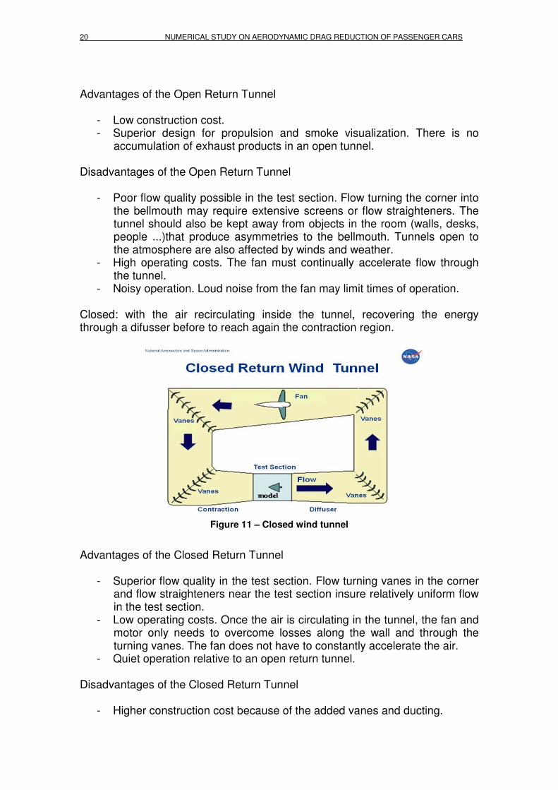
- Noisy operation. Loud noise from the fan may limit times of operation. Closed: with the air recirculating inside the tunnel, recovering the energy through a difusser before to reach again the contraction region.
Figure 11 – Closed wind tunnel
Advantages of the Closed Return Tunnel
- Superior flow quality in the test section. Flow turning vanes in the corner and flow straighteners near the test section insure relatively uniform flow in the test section.
- Low operating costs. Once the air is circulating in the tunnel, the fan and motor only needs to overcome losses along the wall and through the turning vanes. The fan does not have to constantly accelerate the air.
- Quiet operation relative to an open return tunnel. Disadvantages of the Closed Return Tunnel
- Higher construction cost because of the added vanes and ducting.

CHAPTER 4:CAD MODELLING AND CFD SIMULATIONS 21
- Inferior design for propulsion and smoke visualization. The tunnel must be designed to purge exhaust products that accumulate in the tunnel.
- Hotter running conditions than an open return tunnel. Tunnel may have to employ heat exchangers or active cooling.
2.3.2 Flow velocity inside Classification:
- Subsonic - Transonic - Supersonic - Hypersonic
Figure 12 – Classification of wind tunnels
2.4 Components
2.4.1 Fan Produces the air stream in the circuit in which the airflow is developed.
2.4.2 Test Section Where the experimental model to test stands. The size of the Test section is one of the most important characteristics of a wind tunnel; a large one allows testing without large scale reduction from the original, which keeps the index of similarity of Reynolds number.
2.4.3 Stabilizers and Vanes In order to correct the rotation introduced in the flow by the fan.
2.4.4 Windows Windows or vents that allow pressure equalization and prevent critical oscillations on them.

22 NUMERICAL STUDY ON AERODYNAMIC DRAG REDUCTION OF PASSENGER CARS
2.4.5 Diffuser In order to reduce the fluid velocity and recover the static pressure during expansion, the diffuser is divided into two parts by the fan. The difussers are very sensitive to design errors, and can induce separation of the boundary layer in a intermittent or in a stable manner that is very difficult to detect and can create vibrations in the tunnel, swing on the ventilator and variation in the air speed of the test section. The air entering the diffuser is not laminar and the air coming out of the test section is not uniform, both conditions make difficult the work of the diffuser in every the loop.
2.4.6 Contraction cone Its function is to increase the flow velocity. The wind tunnel can be constructed of different materials such as: steel sheet, aluminum, wood, cement, reinforced plastic, etc. However the mixed wood and steel construction finally prevailed, as it is easy to work with and maintain.
2.5 Measurement problems on a wind tunnel
2.5.1 Scale effect limitations These limitations are given by reducing the size of the model. For example: a model of 1: 4 scale, must be tested @ 4 times the actual speed. This shows that as the smaller the model the highest the speed used in the test section, which may be limited by the maximum speed of the tunnel Fan system and/or maximum Power to move the fan. These limitations are canceled if a pressurized tunnel is used.
Power= (2-1) where: A: test section cross section Area U: Flow Velocity.
2.5.2 Model dimensions The aerodynamic researchers must find a compromise between the dimensions of the model and the Tunnel. The decision is rather dictated by cost considerations. Once the Reynolds and Mach numbers can not be reproduced, experimental data is affected by the effects of scale, sometimes it is negligible. In the case of low speed transonic flows, the scale effect is considered.
CHAPTER 4:CAD MODELLING AND CFD SIMULATIONS 23
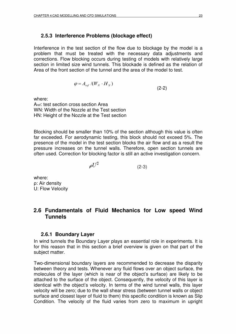
2.5.3 Interference Problems (blockage effect) Interference in the test section of the flow due to blockage by the model is a problem that must be treated with the necessary data adjustments and corrections. Flow blocking occurs during testing of models with relatively large section in limited size wind tunnels. This blockade is defined as the relation of Area of the front section of the tunnel and the area of the model to test.
(2-2)
where: Aref: test section cross section Area WN: Width of the Nozzle at the Test section HN: Height of the Nozzle at the Test section
Blocking should be smaller than 10% of the section although this value is often far exceeded. For aerodynamic testing, this block should not exceed 5%. The presence of the model in the test section blocks the air flow and as a result the pressure increases on the tunnel walls. Therefore, open section tunnels are often used. Correction for blocking factor is still an active investigation concern.
(2-3) where: ρ: Air density U: Flow Velocity
2.6 Fundamentals of Fluid Mechanics for Low speed Wind Tunnels
2.6.1 Boundary Layer In wind tunnels the Boundary Layer plays an essential role in experiments. It is for this reason that in this section a brief overview is given on that part of the subject matter. Two-dimensional boundary layers are recommended to decrease the disparity between theory and tests. Whenever any fluid flows over an object surface, the molecules of the layer (which is near of the object’s surface) are likely to be attached to the surface of the object. Consequently, the velocity of this layer is identical with the object’s velocity. In terms of the wind tunnel walls, this layer velocity will be zero; due to the wall shear stress (between tunnel walls or object surface and closest layer of fluid to them) this specific condition is known as Slip Condition. The velocity of the fluid varies from zero to maximum in upright

24 NUMERICAL STUDY ON AERODYNAMIC DRAG REDUCTION OF PASSENGER CARS
layers. It is this type of layer, formed near the wall of the wind tunnel, known as Boundary Layer, where viscosity plays an important role. It leads to a laminar form at low Re, whereas the flow converts to turbulent flow as Re increase. According to the British physicist and engineer Osborne Reynolds “the general character of motion of fluids in contact with solid surfaces depends on the relation between a physical constant of fluid, and the product of the linear dimensions of space occupied by the fluid, and the velocity”. If Lts complies with the length of test section, Uts complies the velocity of air within the test section, then Reynolds number is shown by Re. Therefore one can rewrite all these parameters in the following Equation:
(2-4a)
(2-4b)
where V is kinetic viscosity (defined as inherent friction of adjoining layers in fluid moving at different velocities).
Figure 13 – Boundary Layer representation (a) Laminar flow (b) turbulent flow
Previous figure shows the height of free stream velocity U from the wall of the wind tunnel. Delta shows de Boundary layer thickness. UL is the wall velocity. Figure (a) shows the laminar flow in the boundary layer, and figure (b) shows the turbulent flow. There are many definitions for Laminar flow. According to Smith “fluid can flow in one of two ways. One is in smooth, layered fashion, in which the streamlines all remain in the same relative position with respect to the other. This type of flow is referred to as laminar flow”. At high Reynold’s numbers the layer of air flow nearest to the wall surface acts like the wall surface. Due to many swirls being formed in this layer, all molecules become amalgamate, moving in an irregular fashion.
2.6.2 The Continuity Equation The mathematical equation that represents the conservation of mass of moving fluid is known as the Continuity Equation. Supposing that a fluid is in motion with speed V, distance s moves as fluid in a time interval of ∆t then s can be calculated as below:

CHAPTER 4:CAD MODELLING AND CFD SIMULATIONS 25
(2-5) Presumed that the fluid is in motion in a tube of a cross sectional area of A, the volume V of the fluid can be expressed at this point as:
(2-6) The mass flow rate of this fluid in the tube can be calculated by the following equation:
(2-7) where ρ is the fluid density. If the mass of the fluid is constant between two points of the tube (without additional fluid between this points), this type of flow is called Steady flow (independent on time). As result the mass flow rate will be constant at both points. This can be expressed in form of the following equation:
(2-8) In the case that the fluid within the tube is incompressible and at low speed, its densities at both points of the tube should be the same. Thus the equation can be written as:
(2-9)
2.6.3 Bernouilli Equation Bernouilli’s Equation basically represents the relation between velocity, density and pressure. Since density is a constant, as explained in previous section, the following equation expresses the relation of pressure and velocity between P2 and the conditions at P1 :
(2-10)
Previous equation rewrite and known as Bernouilli Equation:
(2-11) P1, P2 : Static pressure at point 1 and point 2 V1, V2 : Flow speed at point 1 and point 2 h1, h2 : Height of two ends of the tube at point 1 and point 2 In case that V=0 the pressure at two points is equal. Hence it only appears when the fluid id in motion. If the Bernouilli Equation is expressed in terms of
26 NUMERICAL STUDY ON AERODYNAMIC DRAG REDUCTION OF PASSENGER CARS
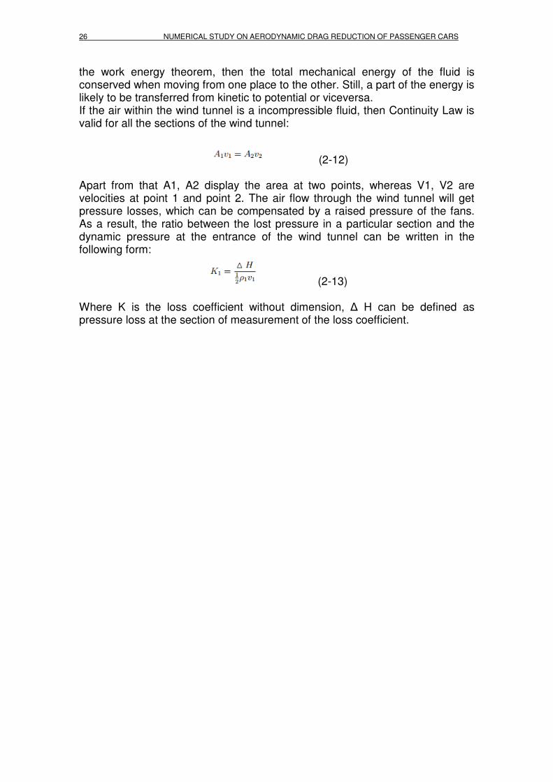
the work energy theorem, then the total mechanical energy of the fluid is conserved when moving from one place to the other. Still, a part of the energy is likely to be transferred from kinetic to potential or viceversa. If the air within the wind tunnel is a incompressible fluid, then Continuity Law is valid for all the sections of the wind tunnel:
(2-12)
Apart from that A1, A2 display the area at two points, whereas V1, V2 are velocities at point 1 and point 2. The air flow through the wind tunnel will get pressure losses, which can be compensated by a raised pressure of the fans. As a result, the ratio between the lost pressure in a particular section and the dynamic pressure at the entrance of the wind tunnel can be written in the following form:
(2-13)
Where K is the loss coefficient without dimension, ∆ H can be defined as pressure loss at the section of measurement of the loss coefficient.

CHAPTER 3:THEORY 27
CHAPTER 3. THEORY In this chapter there is a brief review of the main equations and formulas used for aerodynamic calculations.
3.1 Vehicle aerodynamics All the aerodynamic forces acting on a body is due solely to:
- The distribution of pressure on the surface of the body - The distribution of shear stress on the surface of the body
As you can see in the (Figure 13), the pressure P acts perpendicular to the surface, while the stress τ is tangential to the surface. As explained below, this strain appears as a result of friction between the body and the fluid.
Figure 14 – Pressure and shear over a surface
The distribution of P and τ over the entire surface result in one equivalent force R and moment M. Additionally, the force R can be decomposed into two groups of components, as shown in the picture below (Figure 14).
Figure 15 – Decomposition of R in 2 components
In the image above (Figure 14), V∞ represents the relative wind, which is defined as the flow velocity at infinite. This is called free stream flow (undisturbed flow) and hence V∞ is also called free flow speed.

28 NUMERICAL STUDY ON AERODYNAMIC DRAG REDUCTION OF PASSENGER CARS
Moreover, c is the chord of the profile, defined as the length between the leading edge and trailing edge. Then the angle α is defined as the angle between c and V∞ and it’s called the angle of attack. Regarding the different components of R, by definition:
L = Lift, is the component of R perpendicular to V∞ D = Drag or resistance, is the component of R parallel to V∞ N = Normal, is the component of R perpendicular to c A = Axial, is the component of R parallel to c
The geometric relationships between these four components can be observed in the image above (Figure 14):
L = N cos α – A sin α (3-1) D = N sin α + A cos α (3-2)
Thus, in order to obtain the expressions for Lift and Drag forces is necessary to know previously Normal and Axial forces. N and A are found by integration of pressure and shear stress over the body surfaces.
Figure 16 – Aerodynamic Forces acting on a car
3.1.1 Drag Drag is the aerodynamic force that opposes a vehicle’s motion through the air. Drag is a mechanical force generated by the interaction and contact of a solid
CHAPTER 3:THEORY 29
body with a fluid. It is very important in design of vehicles because the higher this force is, the higher the power needed to move the vehicle.
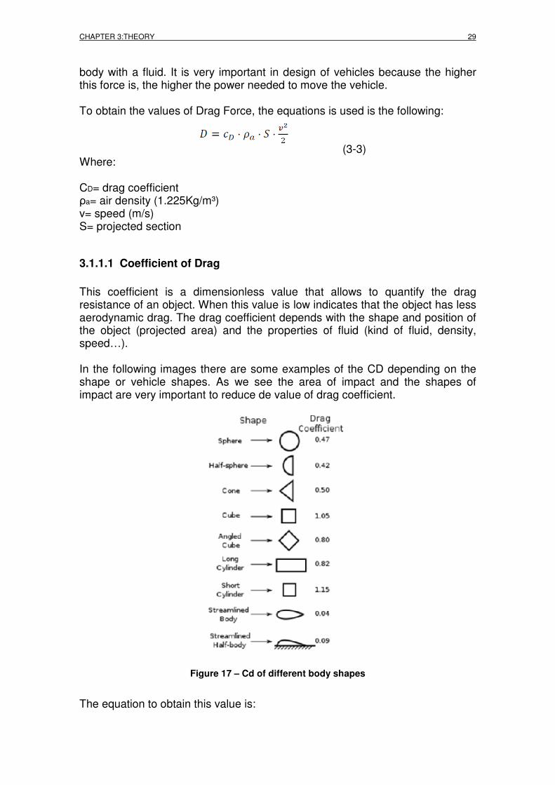
To obtain the values of Drag Force, the equations is used is the following:
(3-3) Where: CD= drag coefficient ρa= air density (1.225Kg/m³) v= speed (m/s) S= projected section
3.1.1.1 Coefficient of Drag This coefficient is a dimensionless value that allows to quantify the drag resistance of an object. When this value is low indicates that the object has less aerodynamic drag. The drag coefficient depends with the shape and position of the object (projected area) and the properties of fluid (kind of fluid, density, speed…). In the following images there are some examples of the CD depending on the shape or vehicle shapes. As we see the area of impact and the shapes of impact are very important to reduce de value of drag coefficient.
Figure 17 – Cd of different body shapes
The equation to obtain this value is:
30 NUMERICAL STUDY ON AERODYNAMIC DRAG REDUCTION OF PASSENGER CARS
(3-4) Where: D= Drag Resistance ρa= air density (1.225Kg/m³) v= speed (m/s) S= projected section
3.1.2 Lift Lift is a force generated by a body that moves that body perpendicular to the direction of incident flow. It is specially used in airplanes to make them fly. It consists in a differential of pressure between the top and the bottom of the wing. These pressures tend to equal, therefore this force (lift) appears that makes to push up the wing and as the result the plane. In our current work, we have a car and the lift is negative to keep the vehicle in contact with the ground. The equation used to obtain the value of Lift is the following:
(3-5) where: CL= Lift coefficient ρa= air density (1.25Kg/m³) v= speed (m/s) S= projected section
CHAPTER 3:THEORY 31
3.1.2.1 Lift coefficient Just as the drag coefficient, the lift coefficient is also a dimensionless value. This is used to know the quantity of force in perpendicular direction that the body receives from the incident flow. The lift coefficient can be expressed as the following equation:
(3-6) where: L= Lift resistance ρa= air density (1.225Kg/m³) v= speed (m/s) S= projected section
3.1.3 Ground effect The ground effect is called to the aerodynamic action when a body has a differential pressure between the top and the bottom of the car. The pressure that appears on the top of the car is higher than the pressure of the ground vehicle, therefore this differential makes car to smash the ground. This effect helps to increase the grip and it allows the car to increase its velocity in corners. This effect is very common in competition cars. Due to the ground effect car can go faster in the turns without losing grip.
3.2 Motor vehicle dynamics
3.2.1 Total Resistance Force Total movement resistance is:
(3-7) FT= Total resistance force [N] RT= Resistance due to mechanical friction of transmission RR= Resistance due to the road friction RA= Resistance due to the air (Drag resistance)
3.2.1.1 Resistance due to the mechanical friction of transmission (RT) This resistance depends on the efficiency of the transmission (ƞtr). This value is about 0.85 and 0.9 [22].

32 NUMERICAL STUDY ON AERODYNAMIC DRAG REDUCTION OF PASSENGER CARS
3.2.1.2 Resistance due to the road friction (RR) The resistance RR is related with the road conditions. Is one of the most important and relevant resistance to the movement of the vehicle. Equation:
(3-8) where: M= mass of the vehicle [kg] g= gravity (9.81 m/s²) f= tread coefficient The f coefficient is a dimensionless coefficient that depends on the road friction coefficient (µr) and the radius of the wheel.
(3-9) This value for a commercial vehicle in a typical road is about 0.006 to 0.010 [23].
3.2.1.3 Resistance due to the air (RA) The resistance due to the aerodynamics is one of the most important factors, and is main study in this work.
(3-10) CD= drag coefficient ρa= air density (1.225Kg/m³) S= projected section v= speed (m/s) The CD coefficient depends on the shape of the car and its accessories. If the drag coefficient increases, it will increase the air resistance. Therefore, the total resistance and the fuel consumption will also increase.
3.2.2 Power In this section the power needed to beat the resistance is going to be reviewed. The force to beat is the addition of the three resistance forces.

CHAPTER 3:THEORY 33
Therefore, we can define this power like the manager to beat the forces in one speed.
(3-11)
(3-12)
(3-13) We consider N like the all the external resistance that affect to the car. PN should be provided by a motor and can be defined with the transmission efficiency. Hence, we can consider the next equation:
(3-14) With this equation, we can obtain the total power needed for the engine. Now, we have to link it with fuel consumption. Therefore, we should define energy consumption per hour (B) [Kg/h] and specific energy consumption (be) [KWh/km].
(3-15)
(3-16)
Figure 18 – Specific energy consumption (for medium size passenger cars) [25]
The total consumption of energy should be defined:
(3-17)

34 NUMERICAL STUDY ON AERODYNAMIC DRAG REDUCTION OF PASSENGER CARS
t= time working
(3-18) d= distance (m) v= velocity (m/s) The next equation is the related velocity and energy consumption:
(3-19) To link the consumption with distance it would be better to define the next equation:
(3-20) However, when we talk about consumption, we are used to use the relation with 100km. Therefore, the equation is the next:
(3-21) The next step is to relate the equations of power with the energy consumption per 100 km.
(3-22)
(3-23) If we put the density of air and we change the specific consumption taking in care the density of the fuel, the final expression is the following:
(3-24)
3.3 CFD
3.3.1 Fluid Dynamics
In this section the theory of the fluid dynamics used in this study is presented. Fluid dynamics describes the motion of fluids in terms of energy, momentum and mass. This study consists of solving the flow around a the Ahmed body by using a commercial CFD software named Ansys Fluent 16. The software solves

CHAPTER 3:THEORY 35
the governing equations for fluid flow dividing the physical domain into small finite volume elements where the governing equations are solved numerically. Almost all flows are turbulent (Re>10^6), so, the turbulence model must be chosen keeping in mind the accuracy and the computational cost of every turbulence model. In the following sections, the governing equations are presented as well as turbulence model.
3.3.2 Governing equations
A first approach for describing the flow field is to state the three laws of conservation. The governing equations are derived from basic physics principles but can not be solved analytically and must be solved by numerical simulations.
3.3.2.1 Conservation of mass Equal amount of mass enters and leaves the Control Volume:
(3-25)
3.3.2.2 Conservation of linear momentum It is the Newton’s Second Law of motion: Relation between pressure, momentum and viscous forces. This set of formulas are referred as the incompressible Navier-Stokes equations which are non-linear partial differential equations:
(3-26)
3.3.2.3 Conservation of Energy It is the First Law of Thermodynamics: The total amount of Energy within the system stays constant:
(3-27)

36 NUMERICAL STUDY ON AERODYNAMIC DRAG REDUCTION OF PASSENGER CARS
3.3.2.4 Navier-Stokes equations Due to the stochastic, three-dimensional, time dependent and turbulent flow, there will be fluctuations within the flow field. To handle this, the Navier-Stokes equations (written under the conservation of linear momentum) must be time-averaged. Assuming incompressible and isothermal flow, the density and viscosity can be seen as constant values. This assumption is possible because our case is under Mach Number < 0.4. Temperature is relatively low during the simulation of the flow field, hence the energy equation can be neglected. Navier-Stokes equations are derived from Newton’s second Law and can be seen as a force of equilibrium for an infinitesimal small volume element. In order to convert the stress to velocity components, the Navier-Stokes are usually expressed for an incompressible Newtonian fluid with constant viscosity. An incompressible fluid is a fluid where the Divergence of the Velocity is zero, and a Newtonian fluid is a fluid which stress versus strain curve is linear. The Navier-Stokes equations can then be expressed as follows (one for each Velocity vector):
(3-28) Since the flow is assumed incompressible, the continuity equation can be written:
(3-29) Together the Navier-Stokes and the continuity equation gives four unknowns u, v, w and p which will be solved with differential equations.
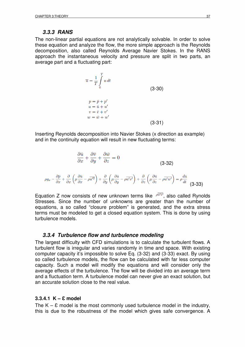
CHAPTER 3:THEORY 37
3.3.3 RANS
The non-linear partial equations are not analytically solvable. In order to solve these equation and analyze the flow, the more simple approach is the Reynolds decomposition, also called Reynolds Average Navier Stokes. In the RANS approach the instantaneous velocity and pressure are split in two parts, an average part and a fluctuating part:
(3-30)
(3-31)
Inserting Reynolds decomposition into Navier Stokes (x direction as example) and in the continuity equation will result in new fluctuating terms:
(3-32)
(3-33)
Equation Z now consists of new unknown terms like , also called Rynolds Stresses. Since the number of unknowns are greater than the number of equations, a so called “closure problem” is generated, and the extra stress terms must be modeled to get a closed equation system. This is done by using turbulence models.
3.3.4 Turbulence flow and turbulence modeling
The largest difficulty with CFD simulations is to calculate the turbulent flows. A turbulent flow is irregular and varies randomly in time and space. With existing computer capacity it’s impossible to solve Eq. (3-32) and (3-33) exact. By using so called turbulence models, the flow can be calculated with far less computer capacity. Such a model will modify the equations and will consider only the average effects of the turbulence. The flow will be divided into an average term and a fluctuation term. A turbulence model can never give an exact solution, but an accurate solution close to the real value.
3.3.4.1 K – Ɛ model The K – Ɛ model is the most commonly used turbulence model in the industry, this is due to the robustness of the model which gives safe convergence. A

38 NUMERICAL STUDY ON AERODYNAMIC DRAG REDUCTION OF PASSENGER CARS
good overview of the flow field is achieved with the model, but in areas with high velocity and pressure gradients, the accuracy is not that high. The K – Ɛ model is an Eddy Viscosity model where the turbulence is modeled by adding turbulence viscosity, . This is a semi empirical method based on how the kinetic energy, k, is transported and its dissipation rate Ɛ. The transport equation for k is derived exact while the transport equation for Ɛ is derived from physical reasoning. The biggest eddies gets the kinetic energy,
() , from the main flow. The energy is transmitted into smaller eddies and ends up as integral energy. Since the K – Ɛ model is a RANS-model and is using time average terms the model will miss differences in the gradients during very short time steps.
3.3.4.2 K – Ɛ Realizable In order to achieve a more accurate solution of the flow, a new model has been developed and called the K – Ɛ Realizable model. This new model has a new formulation for the turbulent viscosity, transport equation and for the dissipation rate. In the derivation of the Standard K – Ɛ model, the flow is assumed to be fully turbulent, which makes the model only valid for these circumstances. In the K – Ɛ Realizable model, the normal and molecular stresses are taken into account only until some extend. The relationship between the kinetic energy, the dissipation rate and the turbulent viscosity is defined in:
(3-34)
As mentioned an extra , is included in the Navier Stokes equation. In the K – Ɛ model the extra estress term is modeled with a Boussinesq assumption:
(3-35)
3.3.5 Boundary Layers and Wall Functions
When a fluid flows along a body, a boundary layer is created near the surface, and there the velocity grows from zero until it reaches de freestream velocity. The thickness of the boundary layer is defined as the distance from the body to where the velocity reaches 99% of the freestream velocity (Prandtl). The boundary layer can be divided into 3 areas, one laminar, one turbulent, and the last as a mixture of both. The boundary layer starts as laminar when the body is exposed to the fluid, as the fluid develops along the body it becomes more and more turbulent. A laminar boundary layer is always preferable since the skin friction is lower compared with a turbulent layer. The near wall flow is usually divided into three regions, the viscous sub-layer, the buffer layer and the fully turbulent log-law region. The following figure shows the near wall region plotted with semi-log coordinates. On the y-axis there is the non-dimensional wall distance y+ which is defined as in equation (3-36)

CHAPTER 3:THEORY 39
Figure 19 – Velocity profile in the boundary layer on a flat plate (Cartesian)
Figure 20 – Velocity profile in the near wall region (logaritmic)
(3-36)
(3-37)
Where u* is the friction velocity, v is the kinematic viscosity and y is the height of the first cell. In fluent there are two types of wall functions, standard wall functions and non equilibrium wall functions. Standard wall functions assume that the flow near the wall behaves fully turbulent and use the algorithm to resolve the gradients in the boundary layer. In the Non-equilibrium wall functions, the sensitivity for pressure gradients is higher than for the standard wall functions. The Non-equilibrium wall functions predict the flow better in domains where the geometry is complex and separation with reattachments frequently appears. When the boundary layer (without standard wall functions) is calculated on the simulation, the following values are required: y+ =1 In this study, in order to solve the velocity profile in the boundary layer, the Non-equilibrium wall functions have been used, and the following values are required: 30< y+ < 300

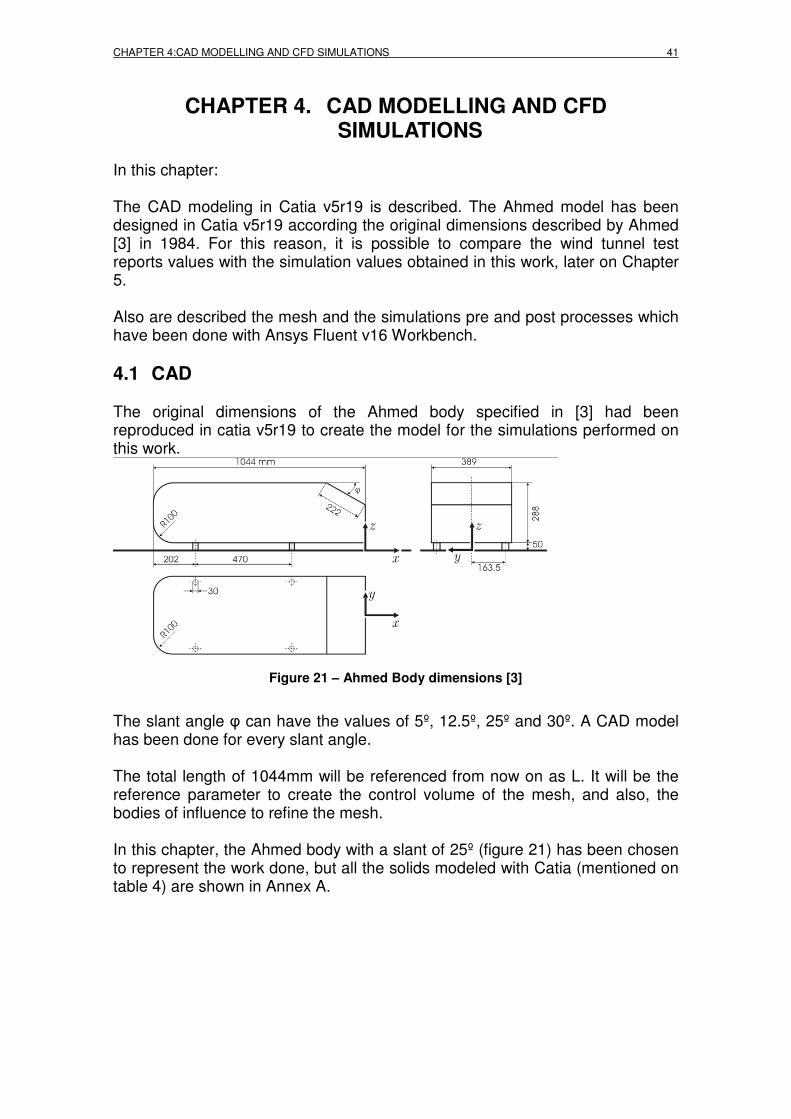
CHAPTER 4:CAD MODELLING AND CFD SIMULATIONS 41
CHAPTER 4. CAD MODELLING AND CFD SIMULATIONS
In this chapter: The CAD modeling in Catia v5r19 is described. The Ahmed model has been designed in Catia v5r19 according the original dimensions described by Ahmed [3] in 1984. For this reason, it is possible to compare the wind tunnel test reports values with the simulation values obtained in this work, later on Chapter 5. Also are described the mesh and the simulations pre and post processes which have been done with Ansys Fluent v16 Workbench.
4.1 CAD The original dimensions of the Ahmed body specified in [3] had been reproduced in catia v5r19 to create the model for the simulations performed on this work.
Figure 21 – Ahmed Body dimensions [3]
The slant angle φ can have the values of 5º, 12.5º, 25º and 30º. A CAD model has been done for every slant angle. The total length of 1044mm will be referenced from now on as L. It will be the reference parameter to create the control volume of the mesh, and also, the bodies of influence to refine the mesh. In this chapter, the Ahmed body with a slant of 25º (figure 21) has been chosen to represent the work done, but all the solids modeled with Catia (mentioned on table 4) are shown in Annex A.

42 NUMERICAL STUDY ON AERODYNAMIC DRAG REDUCTION OF PASSENGER CARS
Figure 22 – Ahmed Body dimensions 25º slant
Ahmed
Body # Slant Difusser
R end
difusser Tail Boat
Pa
ssiv
e F
low
Co
ntr
ol
1 5 º - - -
2 12,5 º - - -
3 25 º - - -
4 30 º - - -
5 25 º 4 º - -
6 25 º 6 º - -
7 25 º 8 º - -
8 25 º 12,5 º - -
9 25 º 6 º 20 -
10 25 º 6 º 35 -
11 25 º 6 º 50 -
12 25 º 6 º 35 5 º
13 25 º 6 º 35 10 º
Pressure Inlet
low
Pressure inlet
high
Act
ive
F lo
w C
on
tro
l
14 25 º 6 35 - 0 º -
15 25 º 6 º 35 - 15 º -
16 25 º 6 º 35 - 30 º -
17 25 º 6 º 35 - 45 º -
18 25 º 6 º 35 - - 0 º
19 25 º 6 º 35 - - 45 º
Table 4 – Models configuration
4.1.1 Solid mechanical properties With the measure inertia tool of Catia v5r19 the solid properties of each model had been obtained. The properties of the solids include:
Volume= [m3] Area [m2] Mass [kg] Density [kg/m3]
Projected Area [mm2]

CHAPTER 4:CAD MODELLING AND CFD SIMULATIONS 43
Center of Gravity: Gx [mm], Gy [mm], Gz [mm] Inertia Matrix G:
GI
GIGI
GIGIGI
G
oz
yzoy
xzxyox
00
02
=
(4-1) Where: IoxG [kg·m2], IoyG [kg·m2], IozG [kg·m2], IxyG [kg·m2], IxzG [kg·m2], IyzG [kg·m2] Principal moments: M1 [kg·m2], M2 [kg·m2], M3 [kg·m2]
Figure 23 – Solid mechanical properties of the Ahmed 25º
The mechanical properties of the model for every configuration are shown in annex A.
4.2 CFD Design Modeler and Meshing process In order to proceed to mesh the models, the geometry in Catia is exported to step format. Even that the last version of Ansys 16 can read the Catia format (CatPart), the step format which is the classical exchange format (as well as iges format) has been used to avoid external links problems. Fluent Germany published a paper [23] explaining the recommendations to define and generate a mesh for ground vehicles simulation. The procedures used on this work follow in detail that recommendations. Before to proceed to create the mesh, a control volume must be created. It will be the domain where the fluid flow will be simulated. The control volume dimensions are referred to n times L. Being L the total length of the Ahmed Body = 1.044 m (figure 20). Total length= 9L Height= 2L Width= 2L

44 NUMERICAL STUDY ON AERODYNAMIC DRAG REDUCTION OF PASSENGER CARS
Figure 24 – Control Volume dimensions (Side View)
Figure 25 – Control Volume dimensions (Front view)
The Ahmed Body geometry is substracted from the Control Volume, and the result is another Control Volume with the same total dimensions as before but with the Ahmed body shape in negative. The surfaces of the negative volume will be used to apply the seeds for the mesh creation. In a first step the surfaces of the Ahmed body are meshed with triangular elements, and then after the full control volume is meshed with tetrahedron elements.
L 3L 5L
2L
2L

CHAPTER 4:CAD MODELLING AND CFD SIMULATIONS 45
Figure 26 – CFD element types
Ansys Fluent mesher generates a first mesh with the following parameters:
Figure 27 – First coarse mesh parameters
Figure 28 – First coarse mesh

46 NUMERICAL STUDY ON AERODYNAMIC DRAG REDUCTION OF PASSENGER CARS
Figure 29 – Zoom of the first coarse mesh
The result is a mesh with 210743 elements and 40303 nodes. The quality parameter selected to check the mesh is the Skewness. It determines how close to ideal (that is, equilateral or equiangular) a face or cell is. Skewness value is 0.79446. Fluent can run the simulations with Skewness values up to 0.95, but the recommendation is to have a mesh between 0.85 and 0.90 as a maximum.
Figure 30 – Skewness of the first coarse mesh attempt
Then after, two sizing functions had been applied to the surfaces of the Control Volume: First sizing applied to the stilts surfaces:
Figure 31 – First sizing applied on the stilt surfaces
Second sizing function applied to the Ahmed body surfaces:

CHAPTER 4:CAD MODELLING AND CFD SIMULATIONS 47
Figure 32 – Second sizing function applied to the Ahmed body surfaces
And the result is a mesh with 982767 elements and 185009 nodes. Skewness value is 0.78896.
Figure 33 – Mesh after surface sizing functions application
Figure 34 – Zoom of the mesh after surface sizing functions application
Figure 35 – Skewness of the mesh without refinements
We are working with half the Ahmed model for computational cost economy. It is possible because there model geometry is symmetric. But we can’t forget to
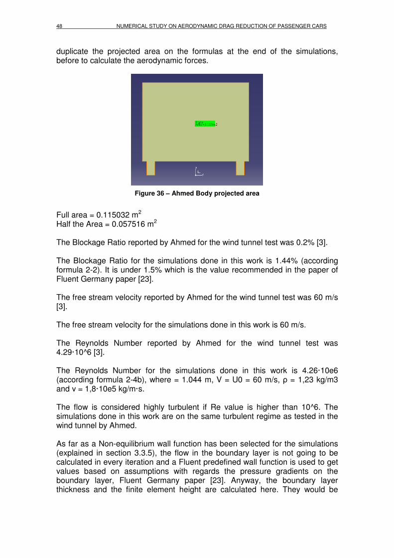
48 NUMERICAL STUDY ON AERODYNAMIC DRAG REDUCTION OF PASSENGER CARS
duplicate the projected area on the formulas at the end of the simulations, before to calculate the aerodynamic forces.
Figure 36 – Ahmed Body projected area
Full area = 0.115032 m2 Half the Area = 0.057516 m2 The Blockage Ratio reported by Ahmed for the wind tunnel test was 0.2% [3]. The Blockage Ratio for the simulations done in this work is 1.44% (according formula 2-2). It is under 1.5% which is the value recommended in the paper of Fluent Germany paper [23]. The free stream velocity reported by Ahmed for the wind tunnel test was 60 m/s [3]. The free stream velocity for the simulations done in this work is 60 m/s. The Reynolds Number reported by Ahmed for the wind tunnel test was 4.29·10^6 [3]. The Reynolds Number for the simulations done in this work is 4.26·10e6 (according formula 2-4b), where = 1.044 m, V = U0 = 60 m/s, ρ = 1,23 kg/m3 and ν = 1,8·10e5 kg/m·s. The flow is considered highly turbulent if Re value is higher than 10^6. The simulations done in this work are on the same turbulent regime as tested in the wind tunnel by Ahmed. As far as a Non-equilibrium wall function has been selected for the simulations (explained in section 3.3.5), the flow in the boundary layer is not going to be calculated in every iteration and a Fluent predefined wall function is used to get values based on assumptions with regards the pressure gradients on the boundary layer, Fluent Germany paper [23]. Anyway, the boundary layer thickness and the finite element height are calculated here. They would be

CHAPTER 4:CAD MODELLING AND CFD SIMULATIONS 49
useful when using standard wall functions and other Turbulence models for simulations: Boundary layer calculation:
δ = L / Re (4-2) δ = 0,000506 m Finite Element height for the boundary layer:
Re1010
Lh ≈≈
δδ
(4-3)
≈δ
h 0,0000506 m
Before to continue with the mesh creation, the relevant surfaces of the control volume have been selected and named. This named surfaces will be automatically detected after by Fluent when it reads the mesh and recognized as No slip walls condition all the symmetry surfaces, except the Ahmed body surfaces and the ground where the inflation will be applied and hence the Non-equilibrium wall functions will be simulated, and also except the Velocity-inlet and the Pressure-outlet that will be recognized as system physical magnitudes inlet and outlet respectively.
Figure 37 – Named Selections
Figure 38 – Ahmed body selection
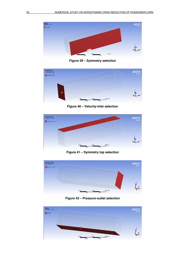
50 NUMERICAL STUDY ON AERODYNAMIC DRAG REDUCTION OF PASSENGER CARS
Figure 39 – Symmetry selection
Figure 40 – Velocity-inlet selection
Figure 41 – Symmetry top selection
Figure 42 – Pressure-outlet selection

CHAPTER 4:CAD MODELLING AND CFD SIMULATIONS 51
Figure 43 – Ground selection
Figure 44 – Symmetry-side selection
The ground surface and the Ahmed body surfaces are specified to be included in the inflation creation. The inflation on the mesh is the creation of a mesh layer for the boundary layer simulation on the surfaces of the Ahmed body and the ground. It will create triangular prism elements along the boundary layer and will keep the rest of the control volume with the tetrahedron elements. The inflation applied is program controlled and the default values proposed by Fluent Germany on document [23] are good enough to perform our simulations. Maximum layer thickness is 5 mm, growth factor of 20% and one maximum of 5 levels.
Figure 45 – Inflation parameters
And the result after inflation is a mesh with 1172873 elements and 341033nodes. And the Skewness value is 0,81528.
Figure 46 – Mesh after inflation

52 NUMERICAL STUDY ON AERODYNAMIC DRAG REDUCTION OF PASSENGER CARS
Figure 47 – Zoom of the mesh after inflation
Figure 48 – Skewness of the mesh after inflation
Now it’s time for mesh refinement. The purpose of mesh refining is to modify the density of elements inside of the control Volume. The objective is to have more accuracy on the calculations (and hence more density of elements) on the areas where the fluid flow is in contact with the Ahmed body relevant surfaces. We are not interested to have a great resolution in the far field for example Velocity inlet and Pressure outlet areas. The strategy for mesh refining chosen for this work is based on internal boxes created around the vehicle and in the wake region to explicitly control mesh size. This approach is more time consuming than other strategies, but is very accurate. The boxes are created in the Preprocessing tool. A constant size of surface elements is applied to the box walls. The boxes are used as meshing domains, in which cell size can be controlled in a very comfortable way. For mesh refining, three boxes have been done to increase the mesh density on the areas of interest. First box, called carbox. It refines the control volume on the sorroundings of all the Ahmed body surfaces in 0.5L on the front of the body, 1L on the rear of the body and 0.25L on the top of the body.

CHAPTER 4:CAD MODELLING AND CFD SIMULATIONS 53
Figure 49 – Carbox
Figure 50 – Carbox sizing function parameters
Mesh after application of the carbox control volume:
Figure 51 – Carbox influence on the mesh
Figure 52 – Zoom of the carbox influence on the mesh

54 NUMERICAL STUDY ON AERODYNAMIC DRAG REDUCTION OF PASSENGER CARS
Figure 53 – Skewness after application of the carbox control volume
Second box, called underbody. It refines the control volume between the ground and the underbody of the Ahmed surfaces. It has a length of 1L, a height of 0.05L and a profundity of 0.3L.
Figure 54 – Underbody
Figure 55 – Underbody sizing function parameters
Figure 56 – Underbody influence on the mesh
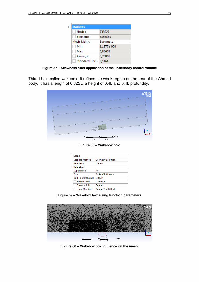
CHAPTER 4:CAD MODELLING AND CFD SIMULATIONS 55
Figure 57 – Skewness after application of the underbody control volume
Thirdd box, called wakebox. It refines the weak region on the rear of the Ahmed body. It has a length of 0.825L, a height of 0.4L and 0.4L profundity.
Figure 58 – Wakebox box
Figure 59 – Wakebox box sizing function parameters
Figure 60 – Wakebox box influence on the mesh

56 NUMERICAL STUDY ON AERODYNAMIC DRAG REDUCTION OF PASSENGER CARS
Figure 61 – Skewness after application of the underbody box control volume
At this point, the mesh has 4409609 elements and 964054 nodes, with a maximum element skewness of 0.813, which is a good value to start the set up process.
4.3 CFD Setup and Boundary Conditions FLUENT is the solver used by ANSYS to simulate the fluid flow conditions in CFD (Computational Fluid Dynamics). It is based on the Finite Volume Method to solve the governing equations of the fluids explained in Section 3.3. After the mesh has been imported in Fluent Ansys, a check has been performed to be sure that there are no negative volumes on the mesh. Check result is successful.
Figure 62 – Mesh check
The set up for all the simulations is the same as described below: The parameters used for the 19 simulations done on this work are detailed in the following screenshots. The reference explained is (same as in the meshing process) the Ahmed body with 25º slant. In the cases where pressure inlet has been used, the set up mandatory changes will be explained at the end of this section. On the assumptions made in 3.3.2.4 the temperature was considered as a constant (288.16 K = 15º C), so the Energy equation is disabled. On the assumptions made in 3.3.2.4 the density was considered as a constant (1,225 kg/m3), so the flow is considered incompressible. Velocity imposed on the inlet 60 m/s. Pressure imposed on the outlet 101.325 Pa.
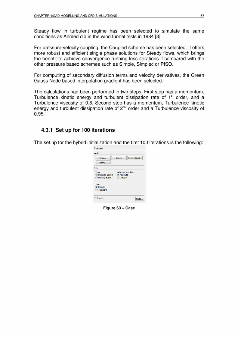
CHAPTER 4:CAD MODELLING AND CFD SIMULATIONS 57
Steady flow in turbulent regime has been selected to simulate the same conditions as Ahmed did in the wind tunnel tests in 1984 [3]. For pressure-velocity coupling, the Coupled scheme has been selected. It offers more robust and efficient single phase solutions for Steady flows, which brings the benefit to achieve convergence running less iterations if compared with the other pressure based schemes such as Simple, Simplec or PISO. For computing of secondary diffusion terms and velocity derivatives, the Green Gauss Node based interpolation gradient has been selected. The calculations had been performed in two steps. First step has a momentum, Turbulence kinetic energy and turbulent dissipation rate of 1st order, and a Turbulence viscosity of 0.8. Second step has a momentum, Turbulence kinetic energy and turbulent dissipation rate of 2nd order and a Turbulence viscosity of 0.95.
4.3.1 Set up for 100 iterations The set up for the hybrid initialization and the first 100 iterations is the following:
Figure 63 – Case

58 NUMERICAL STUDY ON AERODYNAMIC DRAG REDUCTION OF PASSENGER CARS
Figure 64 – Viscous model
The flow joins the Control Volume on the Velocity-inlet, defined during the meshing process. The turbulent intensity has been changed to 1% assuming that the flow is quite laminar at the inlet of the control volume:
Figure 65 – Velocity inlet
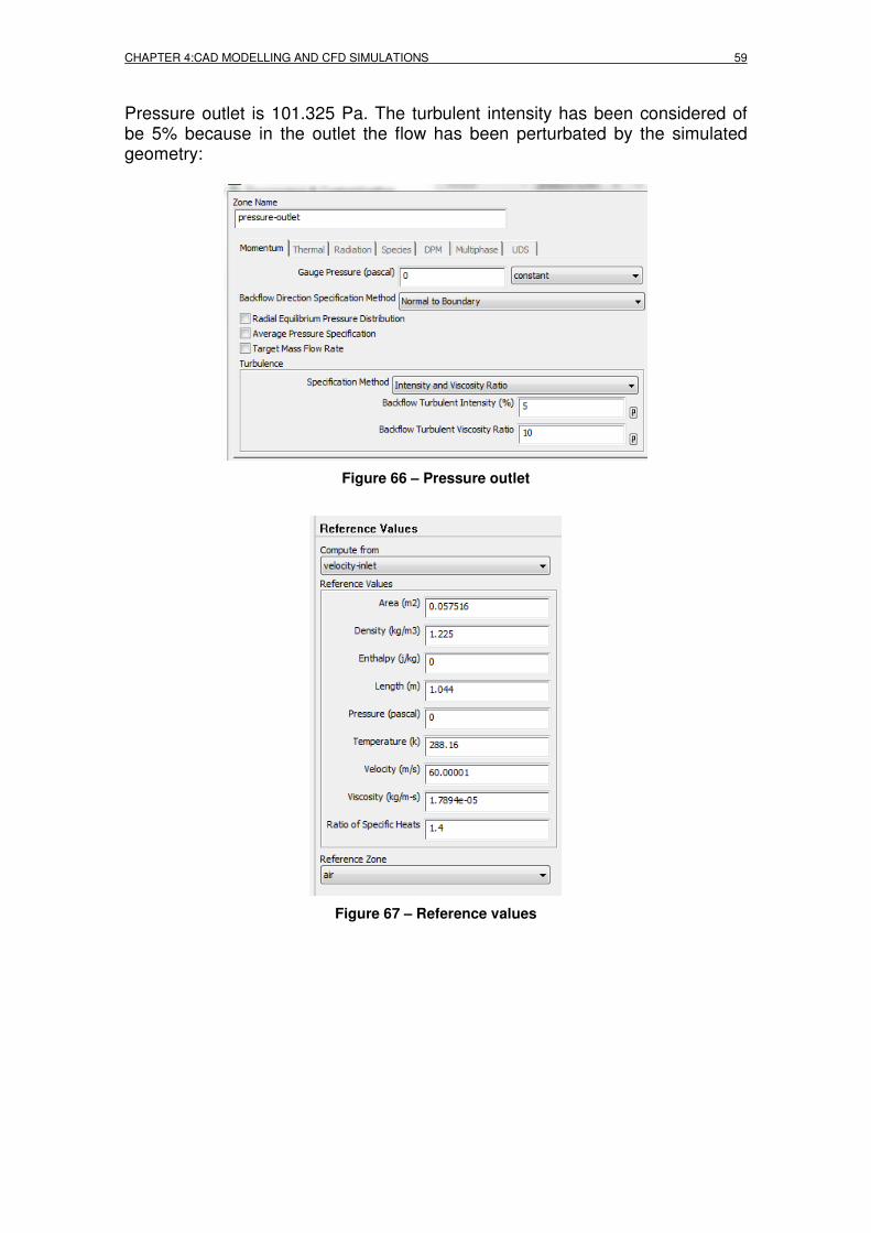
CHAPTER 4:CAD MODELLING AND CFD SIMULATIONS 59
Pressure outlet is 101.325 Pa. The turbulent intensity has been considered of be 5% because in the outlet the flow has been perturbated by the simulated geometry:
Figure 66 – Pressure outlet
Figure 67 – Reference values

60 NUMERICAL STUDY ON AERODYNAMIC DRAG REDUCTION OF PASSENGER CARS
Figure 68 – Solution methods
Figure 69 – Solution controls
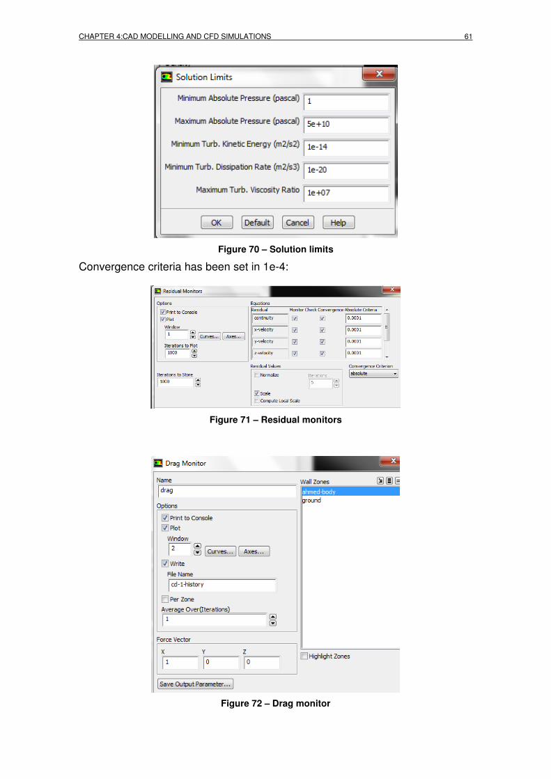
CHAPTER 4:CAD MODELLING AND CFD SIMULATIONS 61
Figure 70 – Solution limits
Convergence criteria has been set in 1e-4:
Figure 71 – Residual monitors
Figure 72 – Drag monitor

62 NUMERICAL STUDY ON AERODYNAMIC DRAG REDUCTION OF PASSENGER CARS
Figure 73 – Lift monitor
Figure 74 – Moment monitor

CHAPTER 4:CAD MODELLING AND CFD SIMULATIONS 63
Figure 75 – Hybrid initialization
Figure 76 – Calculation: 100 iterations
4.3.2 Set up until convergence The set up changes (after the first 100 iterations) to run the simulation until convergence is reached are: Second order has been selected for momentum, Turbulence kinetic energy and turbulent dissipation rate.
Figure 77 – Solution methods

64 NUMERICAL STUDY ON AERODYNAMIC DRAG REDUCTION OF PASSENGER CARS
Turbulence viscosity is set to 0.95:
Figure 78 – Solution controls
Figure 79 – Run calculation
The convergence criteria for the monitors is 1e-4. It means that the solution will be considered converged when the change on the values on the residual of continuity between two consecutive iterations is equal or smaller than 0.0001. Convergence is reached at 381 iterations.
Figure 80 – Residuals plot

CHAPTER 4:CAD MODELLING AND CFD SIMULATIONS 65
Figure 81 – Drag coefficient plot
Figure 82 – Lift coefficient plot
Figure 83 – Moment plot
4.3.3 Pressure inlet additional set up In the cases where pressure inlet has been used, all the set up remains the same as sections 4.3.1 and 4.3.2 except:
- One of the on the Ahmed body surfaces must be split in two surfaces in the model.

66 NUMERICAL STUDY ON AERODYNAMIC DRAG REDUCTION OF PASSENGER CARS
- The new surface must be named in the meshing process as pressure inlet.
- On the pre-process set up, the value of the pressure getting into the control volume through the surface and its spatial orientation must be defined (figure 83) and formula (4-5).
Figure 84 – Pressure inlet
Total pressure (formula 4-4) is composed by the static pressure and the dynamic pressure. As far as the static pressure is a fixed value, the maximum pressure in the system available to be blown on this study is the dynamic pressure (4-5).
(4-4)
(4-5) where, q = dynamic pressure in Pascal ρ = air density in kg/m³ v = fluid velocity in m/s Dynamic pressure is 2205 Pa. For the spatial orientation:
- 0º orientation has a vectorial decomposition of (X=1, Z=0) - 15º orientation has a vectorial decomposition of (X=1, Z=0.26795) - 30º orientation has a vectorial decomposition of (X=1, Z=0.57735) - 45º orientation has a vectorial decomposition of (X=1, Z=1)

CHAPTER 4:CAD MODELLING AND CFD SIMULATIONS 67
4.4 Solutions The solutions for every case of the 19 simulations performed are shown and commented on the Appendix B, but the final configuration (as a result of the iterative design and simulation process, carrying the geometrical parameters with the best values in Drag reduction) will be reviewed in detail on Chapter 5 of this work.


CHAPTER 5: STUDY OF DRAG REDUCTION 69
CHAPTER 5. STUDY OF DRAG REDUCTION In this chapter, the original Ahmed Body geometry with the 4 different slants has been simulated with Ansys Fluent, and the results of the CFD simulations had been compared with the test result values reported by Ahmed [3]. The Pressure coefficient acting on the surfaces of the body has a direct relationship with the turbulence and the boundary layer separation, and a review of the Pressure coefficient on the simulations is done. The objective is to evaluate the impact on the Drag coefficient of the geometrical changes applied on the original Ahmed Body for every different configuration. To reach the objective, a total of 19 simulations with different configurations of the Ahmed body (section 4.1) have been performed, all of them with the set up explained in sections 4.2 and 4.3. As far as there are many different parameters to handle, the development of this study has been done in an iterative way, carrying the geometry modification and its parameter with the best solution on actual iteration, for the next iteration. For information of the configurations mentioned but not explained in this Chapter, check Annex B.
5.1 Ahmed Body
5.1.1 Ahmed Body Wind tunnel vs. CFD: Drag coefficient According Ahmed wind tunnel measurements (1984) the Drag values for the different slant configurations is:
Figure 85 – Drag breakdown for three configurations (Ahmed 1984) [3]
where: Cw = Overall Drag Ck = Front part Cs = Slant rear Cb = Vertical rear end base In this work, the 30º (Low Drag configuration) is not considered. The difference with the High Drag configuration is the addition of a fixed splitter plate vertically on the ground board in the plane of symmetry behind the model. Between the upstream edge of the splitter plate and the model base, a gap of about 25 mm was left free.

70 NUMERICAL STUDY ON AERODYNAMIC DRAG REDUCTION OF PASSENGER CARS
First iteration:
slant 5° 12,5° 25° 30°
Simulation Cd 0,23471 0,23996 0,27966 0,30695
Experimental Cd [3] 0,231 0,23 0,285 0,378
Error [%] 1,61 4,33 -1,87 -18,80
Table 5 – First design iteration Cd results and error calculation
Table 6 – Comparison of Experimental and Simulation Cd values
There is a big difference between the values of the test and the simulation for the 30º slant. The 30º slant angle was reported by Ahmed [3] as the critical angle where the separation of the flow occurs but there is no subsequent reattachment on the slant surface (see the vertical hatched line just on the 30º slant angle on the figure below).
Figure 86 – Variation of Cd of the Ahmed Body with base slant angle (α)

CHAPTER 5: STUDY OF DRAG REDUCTION 71
The simulation results analysis suggest that the software is considering flow reattachment also for the critical 30º slant angle. To check the prediction capability of our numerical method chosen for this work (setup and k- Ɛ Realizable model), an additional simulation has been launch with a slant angle of 35º.
Figure 87 – Velocity streamlines for Ahmed body 25º slant
Figure 88 – Velocity streamlines for Ahmed body 35º slant
The result is that for the 35º slant angle after the flow separation occurs, no re-attachment happens and the wake low pressure region structure changes.
After the comparison between the Wind tunnel test results for different slant angles (published by Ahmed in 1984 [3]) and the results of the CFD simulation (Table above), the slant angle of 25º has been chosen to continue on our iterative study because the CFD simulation results with the RANS two-equation K-Ɛ Realizable turbulence method are reasonable accurate results for the study of Drag (with a reasonable deviation with the wind tunnel test results) for angles smaller than 25º.
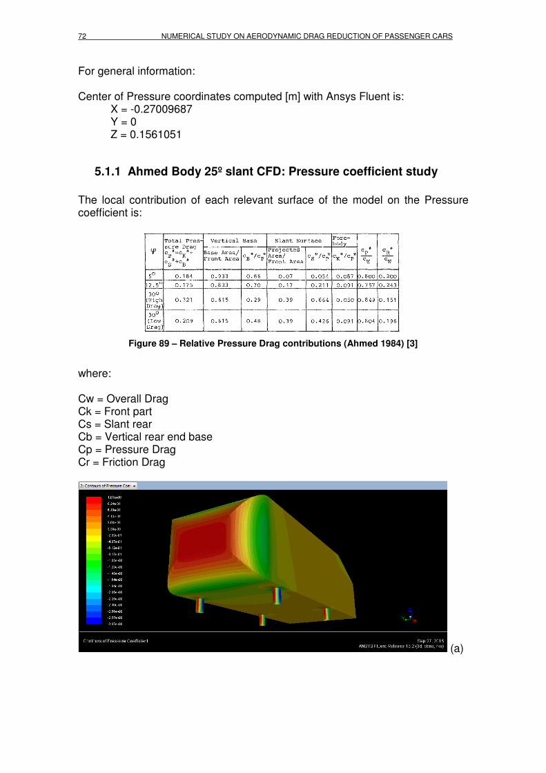
72 NUMERICAL STUDY ON AERODYNAMIC DRAG REDUCTION OF PASSENGER CARS
For general information: Center of Pressure coordinates computed [m] with Ansys Fluent is: X = -0.27009687
Y = 0 Z = 0.1561051
5.1.1 Ahmed Body 25º slant CFD: Pressure coefficient study The local contribution of each relevant surface of the model on the Pressure coefficient is:
Figure 89 – Relative Pressure Drag contributions (Ahmed 1984) [3]
where: Cw = Overall Drag Ck = Front part Cs = Slant rear Cb = Vertical rear end base Cp = Pressure Drag Cr = Friction Drag
(a)

CHAPTER 5: STUDY OF DRAG REDUCTION 73
(b)
Figure 90 – Contours of Pressure coefficient on the Ahmed body 25º surfaces (a) front, (b) rear
And the Pressure coefficient acting on the surfaces of the ahmed body on the symmetry plane can be seen on the following picture:
Figure 91 – Pressure coefficient XY Plot on the symmetry plane of the Ahmed body 25º
slant

74 NUMERICAL STUDY ON AERODYNAMIC DRAG REDUCTION OF PASSENGER CARS
Figure 92 – Pressure coefficient XY Plot on the symmetry plane of the Ahmed body 30º
slant
Figure 93 – Pressure coefficient XY Plot on the symmetry plane of the Ahmed body 35º
slant
When the flow is attached to the surface, the pressure coefficient acting on the surfaces increase, but when it is detached to the surface, the pressure falls and the turbulence Intensity and TKE rise. In reality, the flow detaches at the top edge of the 25º slant, and reattaches to the slant just after the recirculation bubble shown in the figure below:

CHAPTER 5: STUDY OF DRAG REDUCTION 75
Figure 94 – Plot of Ahmed 25º flow reattachment on the 25º slant [27]
To obtain the capture of the real behavior of the flow on the Ahmed body 25º slant with the small recirculation bubble on the top edge of the slant was obtained using the SUPG-PSPG (Streamline Upwind Petrov-Galerkin (SUPG) Pressure Stabilized Petrov Galerkin (PSPG)) scheme. On the following figure, there are a velocity vector plot and a velocity streamlines plot taken from our CFD simulation where no recirculation bubble nor flow reattachment can be seen:
(a)
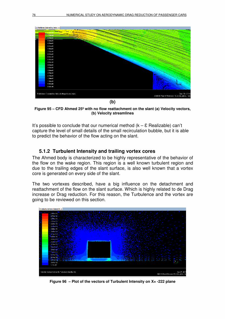
76 NUMERICAL STUDY ON AERODYNAMIC DRAG REDUCTION OF PASSENGER CARS
(b)
Figure 95 – CFD Ahmed 25º with no flow reattachment on the slant (a) Velocity vectors, (b) Velocity streamlines
It’s possible to conclude that our numerical method (k – Ɛ Realizable) can’t capture the level of small details of the small recirculation bubble, but it is able to predict the behavior of the flow acting on the slant.
5.1.2 Turbulent Intensity and trailing vortex cores The Ahmed body is characterized to be highly representative of the behavior of the flow on the wake region. This region is a well known turbulent region and due to the trailing edges of the slant surface, is also well known that a vortex core is generated on every side of the slant. The two vortexes described, have a big influence on the detachment and reattachment of the flow on the slant surface. Which is highly related to de Drag increase or Drag reduction. For this reason, the Turbulence and the vortex are going to be reviewed on this section.
Figure 96 – Plot of the vectors of Turbulent Intensity on X= -222 plane

CHAPTER 5: STUDY OF DRAG REDUCTION 77
Figure 97 – Plot of the vectors of Turbulent Intensity on X= -100 plane
Figure 98 – Plot of the vectors of Turbulent Intensity on X=0 plane
Figure 99 – Plot of the vectors of Turbulent Intensity on X=100 plane

78 NUMERICAL STUDY ON AERODYNAMIC DRAG REDUCTION OF PASSENGER CARS
Figure 100 – Plot of the vectors of Turbulent Intensity on X= 200 plane
Figure 101 – Plot of the vectors of Turbulent Intensity on X= 500 plane
Figure 102 – Plot of the vectors of Turbulent Intensity on X= 750 plane

CHAPTER 5: STUDY OF DRAG REDUCTION 79
Figure 103 – Plot of the vectors of Turbulent Intensity on X= 1000 plane
Figure 104 – Plot of the vectors of Turbulent Intensity on X= 1250 plane
Figure 105 – Plot of the vectors of Turbulent Intensity on X= 1500 plane

80 NUMERICAL STUDY ON AERODYNAMIC DRAG REDUCTION OF PASSENGER CARS
Two counter-rotating trailing vortices are shown in the turbulent kinetic energy (TKE) contour plots. Peaks in TKE occur in the centers of the vortices. These vortices are responsible for maintaining attached flow at the slant up to a slant angle of approximately 30°. A region with high TKE values means a potential region where a vortex core can occur. Derived Landa-2 criterion has been used to check if a vortex core exists. Check value 0.01 [s-²]
Figure 106 – Derived Lambda-2 criteria for Vortex core evaluation (3D)
Vortical structures extend more than 1500 mm beyond the end of the Ahmed body.
5.2 Ahmed Body 25º slant + Diffuser The angle on the rear underbody of the Ahmed body has been studied for 4º, 6º, 8º and 12.5º. It is a primary diffuser shape. An angle of 6º has been chosen as the best value for this stud because, even that Drag reduction is bigger with angles higher than 6º, there are external restrictions for an aerodynamic engineer, and in this case the volume for the car trunk must be respected. Also the exhaust lines with its muffler, the rear suspension and its members, the Fuel Tank and its covers, and finally the differential in case of the all wheel drive versions must be considered.

CHAPTER 5: STUDY OF DRAG REDUCTION 81
Slant 25º + Diffuser 4° 6° 8° 12,5°
Cd 0,2457 0,23634 0,23345 0,20827
Table 7 – Second design iteration Cd results
5.2.1 Pressure coefficient study
Figure 107 – Pressure coefficient XY Plot on the symmetry plane of the Ahmed body 25º slant + 6º diffuser
5.2.2 Turbulent Intensity and trailing vortex cores
Figure 108 – Plot of the vectors of Turbulent Intensity on X= -222 plane

82 NUMERICAL STUDY ON AERODYNAMIC DRAG REDUCTION OF PASSENGER CARS
Figure 109 – Plot of the vectors of Turbulent Intensity on X= -100 plane
Figure 110 – Plot of the vectors of Turbulent Intensity on X=0 plane
Figure 111 – Plot of the vectors of Turbulent Intensity on X=100 plane

CHAPTER 5: STUDY OF DRAG REDUCTION 83
Figure 112 – Plot of the vectors of Turbulent Intensity on X= 200 plane
Figure 113 – Plot of the vectors of Turbulent Intensity on X= 500 plane
Figure 114 – Plot of the vectors of Turbulent Intensity on X= 750 plane
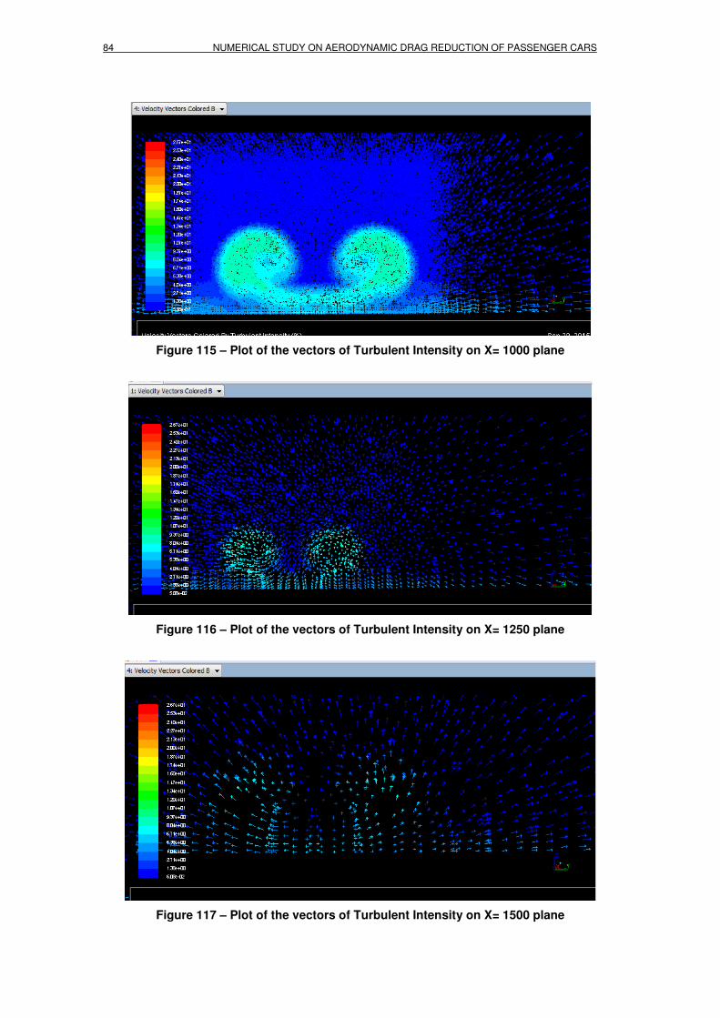
84 NUMERICAL STUDY ON AERODYNAMIC DRAG REDUCTION OF PASSENGER CARS
Figure 115 – Plot of the vectors of Turbulent Intensity on X= 1000 plane
Figure 116 – Plot of the vectors of Turbulent Intensity on X= 1250 plane
Figure 117 – Plot of the vectors of Turbulent Intensity on X= 1500 plane
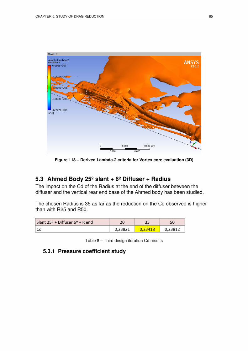
CHAPTER 5: STUDY OF DRAG REDUCTION 85
Figure 118 – Derived Lambda-2 criteria for Vortex core evaluation (3D)
5.3 Ahmed Body 25º slant + 6º Diffuser + Radius The impact on the Cd of the Radius at the end of the diffuser between the diffuser and the vertical rear end base of the Ahmed body has been studied. The chosen Radius is 35 as far as the reduction on the Cd observed is higher than with R25 and R50.
Slant 25º + Diffuser 6º + R end 20 35 50
Cd 0,23821 0,23418 0,23812
Table 8 – Third design iteration Cd results
5.3.1 Pressure coefficient study

86 NUMERICAL STUDY ON AERODYNAMIC DRAG REDUCTION OF PASSENGER CARS
Figure 119 – Pressure coefficient XY Plot on the symmetry plane of the Ahmed body 25º slant + 6º diffuser + Radius 35
5.3.2 Turbulent Intensity and trailing vortex cores
Figure 120 – Plot of the vectors of Turbulent Intensity on X= -222 plane
Figure 121 – Plot of the vectors of Turbulent Intensity on X= -100 plane

CHAPTER 5: STUDY OF DRAG REDUCTION 87
Figure 122 – Plot of the vectors of Turbulent Intensity on X=0 plane
Figure 123 – Plot of the vectors of Turbulent Intensity on X=100 plane
Figure 124 – Plot of the vectors of Turbulent Intensity on X= 200 plane

88 NUMERICAL STUDY ON AERODYNAMIC DRAG REDUCTION OF PASSENGER CARS
Figure 125 – Plot of the vectors of Turbulent Intensity on X= 500 plane
Figure 126 – Plot of the vectors of Turbulent Intensity on X= 750 plane
Figure 127 – Plot of the vectors of Turbulent Intensity on X= 1000 plane

CHAPTER 5: STUDY OF DRAG REDUCTION 89
Figure 128 – Plot of the vectors of Turbulent Intensity on X= 1250 plane
Figure 129 – Plot of the vectors of Turbulent Intensity on X= 1500 plane
Figure 130 – Derived Lambda-2 criteria for Vortex core evaluation (3D)
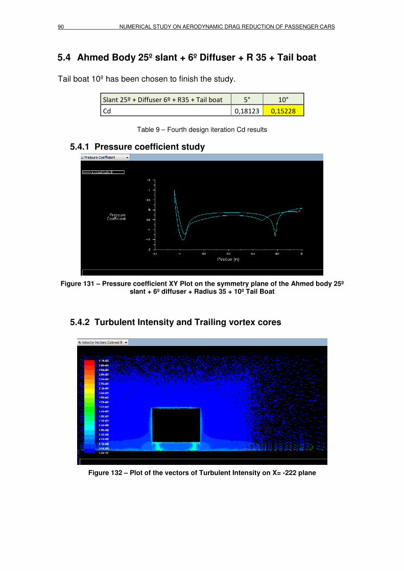
90 NUMERICAL STUDY ON AERODYNAMIC DRAG REDUCTION OF PASSENGER CARS
5.4 Ahmed Body 25º slant + 6º Diffuser + R 35 + Tail boat Tail boat 10º has been chosen to finish the study.
Slant 25º + Diffuser 6º + R35 + Tail boat 5° 10°
Cd 0,18123 0,15228
Table 9 – Fourth design iteration Cd results
5.4.1 Pressure coefficient study
Figure 131 – Pressure coefficient XY Plot on the symmetry plane of the Ahmed body 25º slant + 6º diffuser + Radius 35 + 10º Tail Boat
5.4.2 Turbulent Intensity and Trailing vortex cores
Figure 132 – Plot of the vectors of Turbulent Intensity on X= -222 plane
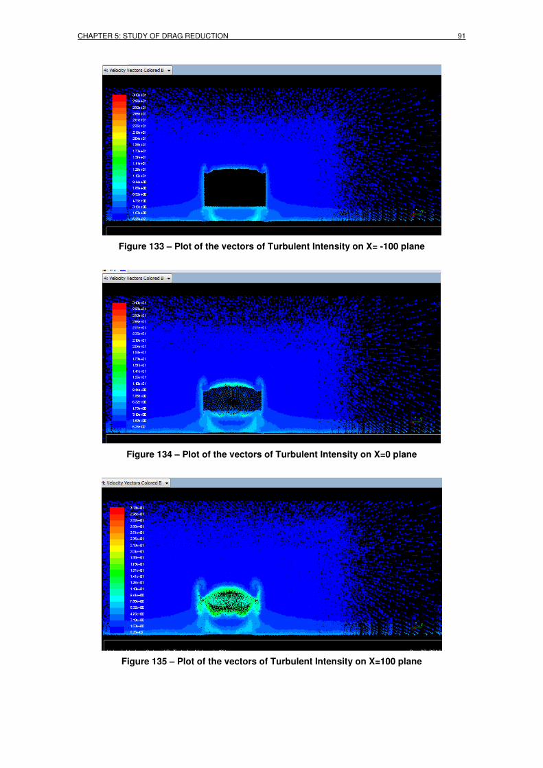
CHAPTER 5: STUDY OF DRAG REDUCTION 91
Figure 133 – Plot of the vectors of Turbulent Intensity on X= -100 plane
Figure 134 – Plot of the vectors of Turbulent Intensity on X=0 plane
Figure 135 – Plot of the vectors of Turbulent Intensity on X=100 plane
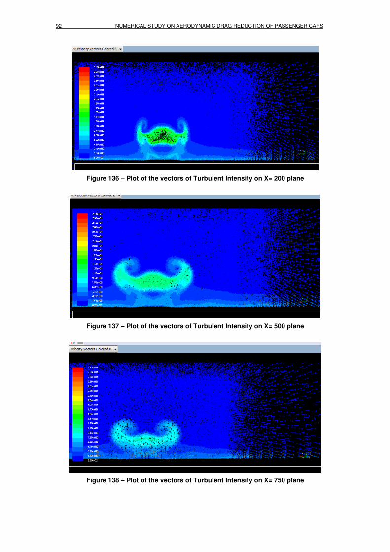
92 NUMERICAL STUDY ON AERODYNAMIC DRAG REDUCTION OF PASSENGER CARS
Figure 136 – Plot of the vectors of Turbulent Intensity on X= 200 plane
Figure 137 – Plot of the vectors of Turbulent Intensity on X= 500 plane
Figure 138 – Plot of the vectors of Turbulent Intensity on X= 750 plane

CHAPTER 5: STUDY OF DRAG REDUCTION 93
Figure 139 – Plot of the vectors of Turbulent Intensity on X= 1000 plane
Figure 140 – Plot of the vectors of Turbulent Intensity on X= 1250 plane
Figure 141 – Plot of the vectors of Turbulent Intensity on X= 1500 plane

94 NUMERICAL STUDY ON AERODYNAMIC DRAG REDUCTION OF PASSENGER CARS
A region with high TKE values means a potential region where a vortex core can occur. Lambda-2 criterion has been used to check if a vortex core exists:
Figure 142 – Derived Landa-2 criteria for Vortex core evaluation (3D)
5.5 Comparison of the Ahmed Body 25º slant and the Ahmed Body 25º slant + 6º Diffuser + R 35 + 10º Tail boat

CHAPTER 5: STUDY OF DRAG REDUCTION 95
(a)
(b)
Figure 143 – Pressure coefficients comparison (a) Ahmed 25º slant, (b) Ahmed 25º slant + 6º diffuser + R35 + 10º Boat tail
5.6 Simulations with Pressure inlet
Active flow control consists to blow air from a surface place of the body (check Annex B for geometric details). In the simulations, two configurations had been studied: low position and high position, with different blowing angles 0º, 15º, 30º and 45º (the reference axis is the direction of the freestream fluid). Check Annex A for simulation result plots. To perform the study, the property imposed on the blowing surfaces is the pressure, 2205 Pa, see section 4.3.3. To understand the table below, the reference Cd value is 0.23669 (Ahmed body with Slant 25º + Diffuser 6º + R 35 end). The impact on the Coefficient of Drag of every configuration is:

96 NUMERICAL STUDY ON AERODYNAMIC DRAG REDUCTION OF PASSENGER CARS
Pressure inlet low 0° 15° 30° 45°
Cd 0,23644 0,23822 0,23487 0,22695
Pressure inlet high 0° 45°
Cd 0,2788 0,23245
Table 10 – Fifth design iteration Cd results
Evaluating the values obtained on the simulations and shown in the table below, is possible to conclude that there is no benefit on Drag reduction with this method as is. The use of high pressure values is needed to have.
5.6.1 Low position
Figure 144 – Pressure inlet surface, low position
5.6.2 High position
Figure 145 – Pressure inlet surface, high position

CHAPTER 6: CONCLUSIONS 97
CHAPTER 6. CONCLUSIONS In this chapter the conclusions are explained, as well as further job is described.
6.1 Aerodynamic analysis conclusions The Coefficient of Drag of the Ahmed body with 25º slant angle has a Cd value of 0.27966, and the Coefficient of Drag of the Ahmed body with 25º slant angle + 6º Diffuser + Radius 35 + 10º Tail boat has a value of 0.15228. The total Cd reduction is 0.12738, and the contribution of each geometric modification on Cd reduction is shown on the following table:
Total Cd reduction Diffuser R TB
Cd reduction contribution 0,12738 0,03925 0,00372 0,08441
[%] 100 30,8 2,9 66,3
Table 11 – Contribution to Cd reduction
It has been noticed that the Radius between the end of the diffuser and the Ahmed’s body back base has a very small influence on the Cd reduction. But the diffuser studied is a primary one with a single angle along its full length. It could be composed of two or more segments with a different angle each, which in combination with the Radius mentioned above, could have a big impact on the Drag coefficient as far as it could increase the velocity of the air exiting the underbody of the body improve the performance of the back. There is a small recirculation region in the upper part of the 25° slant surface reported by [27], and beyond this region the flow reattaches to the slanted surface. This detail is not achieved in the simulation with the k – Ɛ Realizable model but the fluid behavior on the slant is very close to the test condition, and not exceeding the angle value of 25º for the slant design, the simulation set up used in this work is a quick method to estimate the Drag values of a vehicle with small error. There is no benefit observed on Drag reduction by blowing air (2205 Pa, section 4.3.3) from the rear vertical base of the Ahmed body pointing the weak recirculation region of the rear of the body. To obtain benefits with technique, an additional device should be installed in the vehicle to compress air to a magnitude that could affect the Drag coefficient of the vehicle. To obtain such pressure magnitude, the Power required from the engine will increase. It´s not possible to judge in this study, and further work is necessary to evaluate if the net Power increase used to compress the blowing air, is smaller than the reduction on the Power required to beat the Drag Resistance Force, to judge as an efficient method.
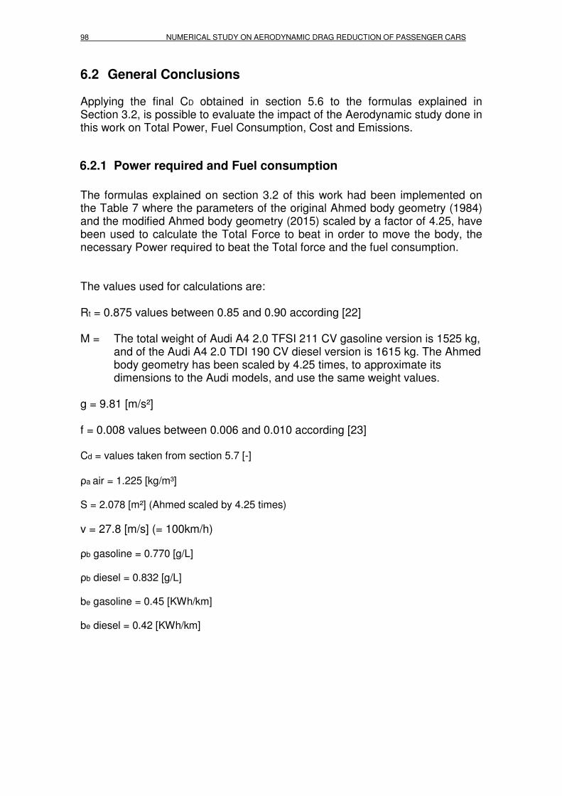
98 NUMERICAL STUDY ON AERODYNAMIC DRAG REDUCTION OF PASSENGER CARS
6.2 General Conclusions Applying the final CD obtained in section 5.6 to the formulas explained in Section 3.2, is possible to evaluate the impact of the Aerodynamic study done in this work on Total Power, Fuel Consumption, Cost and Emissions.
6.2.1 Power required and Fuel consumption The formulas explained on section 3.2 of this work had been implemented on the Table 7 where the parameters of the original Ahmed body geometry (1984) and the modified Ahmed body geometry (2015) scaled by a factor of 4.25, have been used to calculate the Total Force to beat in order to move the body, the necessary Power required to beat the Total force and the fuel consumption. The values used for calculations are: Rt = 0.875 values between 0.85 and 0.90 according [22] M = The total weight of Audi A4 2.0 TFSI 211 CV gasoline version is 1525 kg,
and of the Audi A4 2.0 TDI 190 CV diesel version is 1615 kg. The Ahmed body geometry has been scaled by 4.25 times, to approximate its dimensions to the Audi models, and use the same weight values.
g = 9.81 [m/s²] f = 0.008 values between 0.006 and 0.010 according [23] Cd = values taken from section 5.7 [-]
ρa air = 1.225 [kg/m³] S = 2.078 [m²] (Ahmed scaled by 4.25 times)
v = 27.8 [m/s] (= 100km/h) ρb gasoline = 0.770 [g/L] ρb diesel = 0.832 [g/L] be gasoline = 0.45 [KWh/km] be diesel = 0.42 [KWh/km]
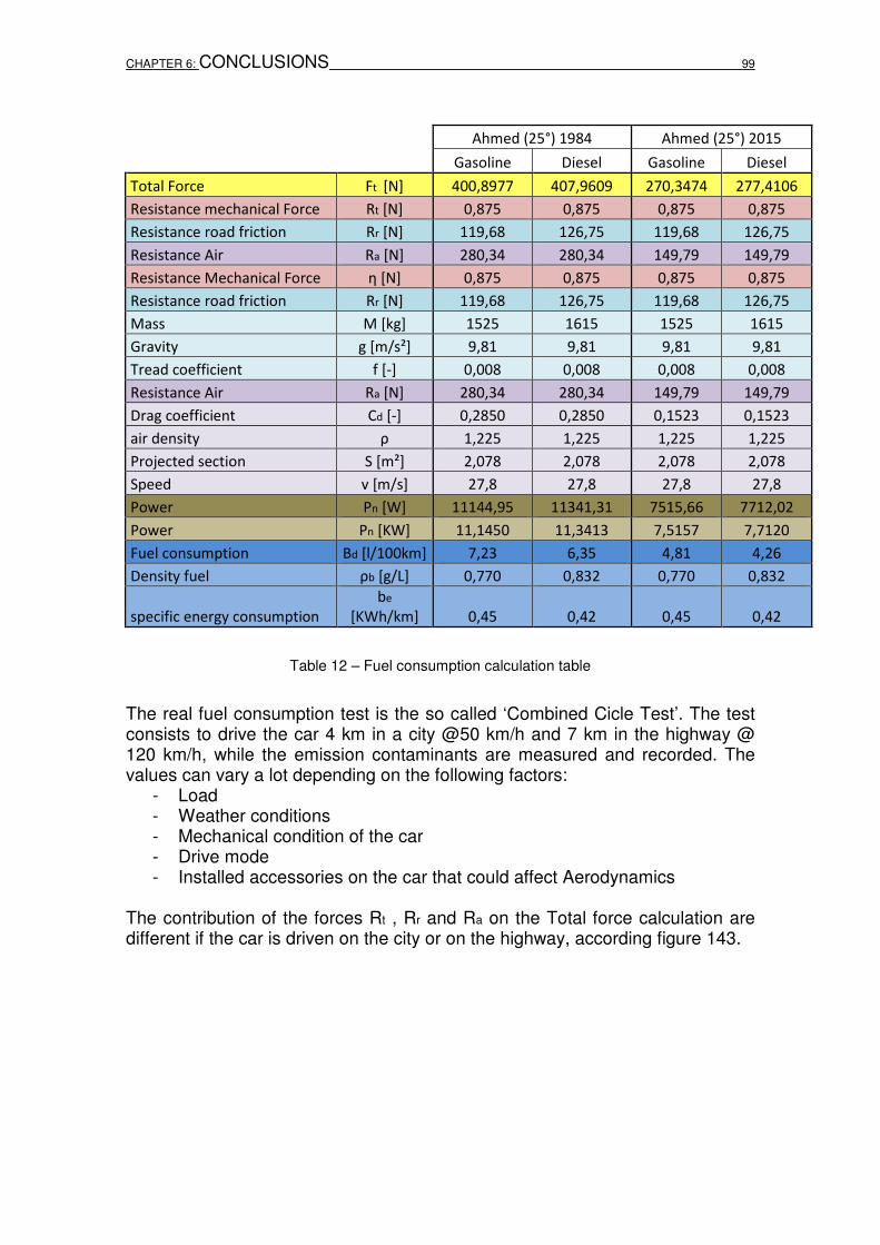
CHAPTER 6: CONCLUSIONS 99
Ahmed (25°) 1984 Ahmed (25°) 2015
Gasoline Diesel Gasoline Diesel
Total Force Ft [N] 400,8977 407,9609 270,3474 277,4106
Resistance mechanical Force Rt [N] 0,875 0,875 0,875 0,875
Resistance road friction Rr [N] 119,68 126,75 119,68 126,75
Resistance Air Ra [N] 280,34 280,34 149,79 149,79
Resistance Mechanical Force η [N] 0,875 0,875 0,875 0,875
Resistance road friction Rr [N] 119,68 126,75 119,68 126,75
Mass M [kg] 1525 1615 1525 1615
Gravity g [m/s²] 9,81 9,81 9,81 9,81
Tread coefficient f [-] 0,008 0,008 0,008 0,008
Resistance Air Ra [N] 280,34 280,34 149,79 149,79
Drag coefficient Cd [-] 0,2850 0,2850 0,1523 0,1523
air density ρ 1,225 1,225 1,225 1,225
Projected section S [m²] 2,078 2,078 2,078 2,078
Speed v [m/s] 27,8 27,8 27,8 27,8
Power Pn [W] 11144,95 11341,31 7515,66 7712,02
Power Pn [KW] 11,1450 11,3413 7,5157 7,7120
Fuel consumption Bd [l/100km] 7,23 6,35 4,81 4,26
Density fuel ρb [g/L] 0,770 0,832 0,770 0,832
specific energy consumption
be
[KWh/km] 0,45 0,42 0,45 0,42
Table 12 – Fuel consumption calculation table
The real fuel consumption test is the so called ‘Combined Cicle Test’. The test consists to drive the car 4 km in a city @50 km/h and 7 km in the highway @ 120 km/h, while the emission contaminants are measured and recorded. The values can vary a lot depending on the following factors:
- Load - Weather conditions - Mechanical condition of the car - Drive mode - Installed accessories on the car that could affect Aerodynamics
The contribution of the forces Rt , Rr and Ra on the Total force calculation are different if the car is driven on the city or on the highway, according figure 143.
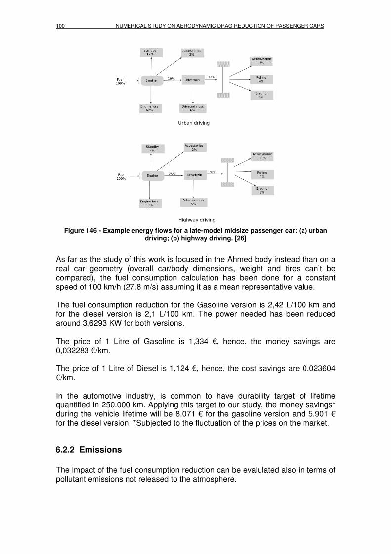
100 NUMERICAL STUDY ON AERODYNAMIC DRAG REDUCTION OF PASSENGER CARS
Figure 146 - Example energy flows for a late-model midsize passenger car: (a) urban driving; (b) highway driving. [26]
As far as the study of this work is focused in the Ahmed body instead than on a real car geometry (overall car/body dimensions, weight and tires can’t be compared), the fuel consumption calculation has been done for a constant speed of 100 km/h (27.8 m/s) assuming it as a mean representative value. The fuel consumption reduction for the Gasoline version is 2,42 L/100 km and for the diesel version is 2,1 L/100 km. The power needed has been reduced around 3,6293 KW for both versions. The price of 1 Litre of Gasoline is 1,334 €, hence, the money savings are 0,032283 €/km. The price of 1 Litre of Diesel is 1,124 €, hence, the cost savings are 0,023604 €/km. In the automotive industry, is common to have durability target of lifetime quantified in 250.000 km. Applying this target to our study, the money savings* during the vehicle lifetime will be 8.071 € for the gasoline version and 5.901 € for the diesel version. *Subjected to the fluctuation of the prices on the market.
6.2.2 Emissions The impact of the fuel consumption reduction can be evalulated also in terms of pollutant emissions not released to the atmosphere.

CHAPTER 6: CONCLUSIONS 101
The most harmful pollutants are CO2 and NOx. The impact on CO2 emission reduction can be calculated because it depends on the fuel consumption. But we can’t calculate the impact on NOx emission reduction, as far as it depends on the combustion processes (such as volume of air in the cylinders, high temperatures and pressure values during combustion. The NOx emission target values specified in the European Emission Standard ‘Euro 6’ can be only obtained by the use of additional devices such as NOx Catalytic Converters and Dust Particle Filters.
6.2.2.1 CO2 The production of CO2 is: 2,370 kg CO2 for every liter of gasoline burned, and 2,650 kg CO2 for every liter of diesel burned. For gasoline engines:
Ahmed (1984): 7,23 l/100 km= 0,0723 l/km 0,0723l/km * 2,370 kgCO2/l = 171,35 gCO2/km Ahmed (2015): 4,81 l/100 km= 0,0481 l/km 0,0481l/km * 2,370 kg CO2/l = 114 gCO2/km Reduction in CO2 emissions = 57,35 gCO2/km
For diesel engines:
Ahmed (1984): 6,35 l/100 km= 0,0635 l/km 0,0635l/km * 2,650 kgCO2/l = 168,275 gCO2/km Ahmed (2015): 4,26 l/100 km= 0,0426 l/km 0,0426l/km * 2,650 kg CO2/l = 112,890 gCO2/km
Reduction in CO2 emissions = 55,385 gCO2/km
For reference: In the Euro 6 standard, the total amount of CO2 emissions allowed for passenger cars with gasoline and diesel engines is 130g CO2/km. This value must be achieved as the total emission mean of the full fleet of the brand.
6.3 Further job The Ahmed Model let us understand the behavior of the fluid around a passenger vehicle but the results of the present work must be understood as a design general guideline (qualitative). Once the results are evaluated as an effective Drag reduction, the geometric modifications with accurate design details should be applied in a model such as one of the DrivAer reference models reviewed in Section 1.4 of this document, to get accurate results (quantitative) and be able to evaluate the impact on power required, fuel consumption and emission reduction.

102 NUMERICAL STUDY ON AERODYNAMIC DRAG REDUCTION OF PASSENGER CARS
Study of Active flow control surfaces to act on the turbulent flow of the rear vertical base of the body and development of devices to achieve the theoretical benefits.

BIBLIOGRAPHY 103
BIBLIOGRAPHY [1] Hucho, W. H. and Sovran, G. (1993) Aerodynamics of road vehicles, Annual Review of Fluid Mechanics. Vol. 25(1), pp485-537. [2] Cooper, K. R. (1993). Bluff body aerodynamics as applied to vehicles. Journal of Wind Engineering and Industrial Aerodynamics, 49, pp. 1-22. [3] Ahmed, S.R., Ramm, G. and Faltin, G. (1984) Some salient features of the time averaged ground vehicle wake. SAE Technical Paper Series, 840300. [4] Morelli, A., Fioravanti, L., and Cogotti, A. (1976). The Body Shape of Minimum Drag. SAE Technical Paper 760186. [5] Le Good, G. M., and Garry, K. P. (2004) On the Use of Reference Models in Automotive Aerodynamics. SAE Technical Paper 2004-01-1308, doi: 10.4271/2004-01-1308. [6] Angelina I. Heft, Thomas Indinger and Nikolaus A. Adams. (2012) Introduction of a New Realistic Generic Car Model for Aerodynamic Investigations. Technische Universität München. [7] M. N. Sudin. (2014) Review of Research on Vehicles Aerodynamic Drag Reduction Methods. University of Malacca. [8] Bayraktar, I., Landman, D., and Baysal, O. (2001). Experimental and Computational Investigation of Ahmed Body for Ground Vehicle Aerodynamics. SAE Technical Paper 2001-01-2742. [9] Krajnovi´c, S., and Davidson, L. (2004). Large-Eddy Simulation of the Flow Around Simplified Car Model. 2004 SAE World Congress, SAE Paper No. 2004-01-0227, Detroit. [10] H. Lienhart and S. Becker. (2003). Flow and turbulent structure in the wake of a simplified car model. SAE Paper 2003-01-0656. [11] Kapadia, S., Roy, S. (2003). Detached Eddy Simulation over a reference Ahmed car model. AIAA Paper 2003-0857. [12] Lanfrit, M. (2005). Best practice guidelines for handling Automotive External Aerodynamics with FLUENT. (Version 1.2), Fluent Deutschland GmbH. [13] Braun, M., Lanfrit, M. (2001). Simulation of the Ahmed Body. 9th ERCOFACT/IAHR Workshop on Refined Turbulence Modelling. [14] Morelli, A. (2000). A New Aerodynamic Approach to Advanced Automobile Basic Shapes. SAE Technical Paper 2000-01-0491.

104 NUMERICAL STUDY ON AERODYNAMIC DRAG REDUCTION OF PASSENGER CARS
[15] Peterson, R.L. (1981). Drag reduction by the addition of a boat-tail to a box shaped vehicle. NASA contractor report 163113. [16] Maji, S. and Almadi, H. (2007). Development of Aerodynamics of a Super Mileage Vehicle. SAE Technical Paper 2007-26-060, 2007, doi: 10.4271/2007-26-060. [17] Guo, L., Zhang, Y., & Shen, W. (2011). Simulation Analysis of Aerodynamics Characteristics of Different Two-Dimensional Automobile Shapes. Journal of Computers, 6(5), 999-1005. doi:10.4304/jcp.6.5.999-1005. [18] Hu, X., Zhang, R., Ye, J., Yan, X., and Zhao, Z. (2011). Influence of Different Diffuser Angle on Sedan's Aerodynamic Characteristics. Physics Procedia, Volume 22, 2011, Pages 239-245. [19] Gustavsson, T. (2006). Alternative approaches to rear end drag reduction. KTH, Department of Aeronautical and Vehicle Engineering, Royal Institute of Technology, TRITA-AVE 2006:12. [20] Han, T., Hammond, D. C., and SAGI, C. J. (1992). Optimization of bluff body for minimum drag in ground proximity. AIAA Journal, Vol. 30, No. 4 (1992), pp. 882-889. [21] Muyl, F., Dumas, L., & Herbert, V. (2004). Hybrid method for aerodynamic shape optimization in automotive industry. Computers & Fluids, 33(5), 849-858. [22] Ricardo A. Marchense, Marcos A. Golato. (2011) El consumo de Combustible y Energía en el transporte. Facultad de Ciencias Exactas y Tecnología, Unversidad Nacional de Tucumán, Argetina. [23] Bosch Inc. (2011). Bosch Automotive Handbook. Bentley Publishers [24] Marco Lanfrit. (2005). Best practice guidelines for handling Automotive External Aerodynamics with FLUENT. Fluent Deutschland GmbH. [25] G. Pistoia. (2010). Electric and Hybrid Vehicles: Power Sources, Models, Sustainability. Elsevier. [26] National Research council. (2006). Transportation Research Board Special Report 286 Tires and Passenger Vehicle Fuel Economy. [27] Gerardo Franck, Fernando Carazo, Norberto Nigro, Mario Storti, Jorge D’El´ıa (2004). SIMULACION NUMERICA DEL FLUJO ALREDEDOR DEL MODELO DE AHMED PARA UN ANGULO DE INCLINACION CRITICO. Universidad del Litoral.

BIBLIOGRAPHY 105
Web References
http://www.cfd-online.com (Visited August and September 2015)
http://en.wikipedia.org/wiki/Main_Page (Visited August and September 2015)
http://www.nasa.gov/centers/glenn/home/index.html (Visited August and September 2015)
http://www.arpem.com/audi/a4/coches/a4-2-0-tdi-190-cv-clean-diesel.html (Visited August and September 2015)
http://www.arpem.com/audi/a4/coches/a4-2-0-tfsi-211-cv.html (Visited August and September 2015)


¡Error! No se encuentra el origen de la referencia.: ¡Error! No se encuentra el origen de la referencia. 107


![ESTUDIO: EVEREG - Profilaxis - CRF DESCRIPTIVO€¦ · [ ] optilene lp [ ] optilene mesh elastic [ ] premilene mesh [ ] c-qur centrifx [ ] premilene mesh plug [ ] safil mesh [ ] optilene](https://static.fdocumento.com/doc/165x107/606fa2552b36203c4a362a62/estudio-evereg-profilaxis-crf-descriptivo-optilene-lp-optilene-mesh.jpg)