


Idiomas
Páginas
Jurídico


Dedicated to people who believes that We must stand together...
[1]


Acknowledgements
A la vida y a la tierra por haberme permitido tener esta aventura y
haber podido ver otro tipo de atardeceres.
A mi madre y a mi esposa por su amor, que lo es todo para mı.
A mis amigos y al resto de mis seres queridos, que sin ellos la vida no
tendrıa sentido.
A mi Ecuador y en especial a mi Quito por ser la tierra que me dio la
vida.
A mi Huelva y Letonia querida, y a su gente por haberme acogido
como en casa.
Y no podrıa faltar, a mis amigos quienes me ayudaron a terminar este
trabajo, Angel, Antonio y Jose Enrique.
A todos ellos, gracias. . . .
Andres
October 2014

Abstract
The energy consumption and the growth of the CO2 emissions related
with the growth of the economy represents a challenge requiring a deep
analysis and the development of appropriated policies. Several ana-
lysis of future changes of the economy of particular countries rely on
quantitative point forecasts for which is difficult to achieve a reason-
able accuracy. In this dissertation a System Dynamics (SD) model,
combined with the design of a set of scenarios, has been developed
and applied to Ecuador within a medium term (up to 2025), allowing
to estimate the Gross Domestic Product (GDP) and the CO2 emissions,
among other variables.
This research applied a combination of the so called decomposition
analysis with a scenario analysis to identify and determine the driv-
ing forces of change of CO2 emissions in Ecuador. A historical, from
1980 to 2010, and a forecast period, from 2011 to 2025, have been con-
sidered. Logarithmic Mean Divisia Index (LMDI) to carry out the de-
composition analysis has been applied to both the historical and fore-
cast periods, using in the latter case different plausible scenarios of
development.
The historical analysis provides insights at both macro and sectoral
level, allowing to establish the driving forces of the system: structure,
scale, energy mix and, energy intensity. The macro decomposition was
based on an extended Kaya identity while the sectoral decomposition
tried to offer deeper insights of each productive sector. In addition,
the formation of a GDP that depends on renewable energy, which in-
troduces a feedback mechanism in the model, has been introduced to
build the model, which allows to generate a non-trivial evolution of the
system.
The four considered scenarios show different emission trajectories,
based on the different alternative development paths. In particular, spe-
cial attention was paid to the effect of a reduction of the share of fossil
energy, as well as of an improvement in the efficiency of the fossil en-
ergy use. The estimated values (for CO2 emission and GDP, among
others) are given in an aggregate way as well as in terms of sectoral
contributions.
In a deeper analysis of the model outcome, we have studied the En-
vironmental Kuznets Curve (EKC) hypothesis for Ecuador in a forth-
coming period, 2011-2025 using the proposed scenarios. Our proposal
goes a step further than previous contributions, and intends to see un-
der which conditions a country could approach the fulfilment of this
hypothesis in the medium term. The results do not support the ful-
filment of the EKC, nevertheless, the estimations show that Ecuador
could be on the way to achieving environmental stabilization in the
near future. Indeed, our estimates show that Ecuador could be able
to enter the area of environmental stability (second stage of the EKC)
in the medium term (2019-2021). However, to achieve this goal it is
essential to implement policies that allow the diversification of energy
sources and to increase the energy efficiency in the productive sectors
in order to get a more sustainable development.
The final conclusion of this work suggests that emissions can evolve
with values higher or lower than the present ones and they will be de-
termined not only by the evolution of the economic growth but also by
the development path. Within the development path, economic growth
interacts with governance, societal choices and other driving forces.
Resumen
El consumo de energıa y el aumento de las emisiones de CO2 relacio-
nadas con el crecimiento economico suponen un desafıo para el desa-
rrollo sostenible que requiere un analisis profundo y el desarrollo de
polıticas apropiadas. Muchos de los analisis de los futuros cambios en
la economıa de paıses o de regiones concretas se basan en prediccio-
nes cuantitativas para las cuales es complicado garantizar una precision
adecuada. En la presente investigacion, se ha construido un modelo uti-
lizando para ello la tecnica de Dinamica de Sistemas (DS) en base a un
enfoque de escenarios que permiten realizar estimaciones, a medio pla-
zo (hasta 2025), del Producto Interno Bruto (PIB) y de las emisiones
de CO2, entre otras variables, para el caso de Ecuador.
Esta investigacion aplica una combinacion del analisis de descomposi-
cion y del analisis de escenarios para identificar y analizar las fuerzas
impulsoras que provocan el cambio de las emisiones de CO2 en Ecua-
dor. Se ha considerado para ello el periodo historico de 1980 a 2010
y una proyeccion hasta el ano 2025. Para el analisis de descomposi-
cion se uso el metodo de Indice de Divisia de la Media Logarıtmica
(IDML), aplicandolo tanto al periodo de datos (1980-2010) como al
periodo de proyeccion (2011-2025), para el cual se emplearon diferen-
tes escenarios que permitıan explorar diferentes formas de desarrollo
en Ecuador.
El analisis historico da una vision a nivel macro a la vez que sectorial,
permitiendo diferenciar diferentes fuentes de cambio: estructurales, de
escala, de mix energetico, y de la intensidad energetica. La descompo-
sicion a nivel macroeconomico se basa en una identidad Kaya exten-
dida, mientras que el analisis sectorial intenta ofrecer una vision mas
profunda de cada sector productivo. Ademas, se ha considerado en el
modelo un enfoque de la formacion del PIB que depende de la energıa
renovable, lo que introduce un mecanismo de retroalimentacion en el
modelo y nos permite generar una evolucion no trivial del sistema.
Los cuatro escenarios que se consideran muestran diferentes patrones
de evolucion de las emisiones de CO2, basados en los diferentes cami-
nos de desarrollo alternativo considerados. En particular, se presto es-
pecial atencion al efecto de la reduccion de la cuota de energıa fosil,
ası como a la mejora en la eficiencia del uso de este tipo de energıa.
Los resultados se dan tanto en forma global para el paıs, como tam-
bien referidos a cada una de los sectores productivos. Se observo que
el efecto de la reduccion de uso de energıa fosil puede ser igual de
efectivo que el aumento de su eficiencia de uso.
En un analisis mas profundo de los resultados del modelo, se ha estu-
diado la hipotesis de la Curva de Kuznets Ambiental (CKA), utilizando
para ello los mismos escenarios referidos anteriormente. Nuestra pro-
puesta va un paso mas alla de las contribuciones anteriores presentes
en la literatura revisada, y tiene la intencion de ver en que condiciones
un paıs podrıa acercarse al cumplimiento de esta hipotesis en el me-
dio plazo. Los resultados no apoyan el cumplimiento de la CKA, sin
embargo, las estimaciones muestran que Ecuador podrıa estar en el ca-
mino de lograr la estabilizacion de las emisiones de CO2 (en relacion
al crecimiento del PIB) en un futuro relativamente cercano. De hecho,
nuestras estimaciones muestran que Ecuador podrıa entrar en el ambi-
to de la estabilidad ambiental (segunda etapa de la CKA) en torno a
2019-2021. Sin embargo, para lograr dicho objetivo, es necesario im-
plementar polıticas que permitan la diversificacion de las fuentes de
energıa y aumentar la eficiencia energetica en los sectores productivos
con el fin de conseguir un desarrollo mas sostenible.
La conclusion final de este trabajo sugiere que las emisiones de CO2
pueden evolucionar a lo largo de diferentes trayectorias, con niveles

de emisiones superiores o inferiores a los actuales, que vendran de-
terminados no solo por la evolucion del crecimiento economico, sino
tambien por la vıa de desarrollo seleccionada. En el camino hacia el
desarrollo, el crecimiento economico interactua con la gobernanza, las
opciones sociales y las otras fuerzas impulsoras.

Contents
List of Figures xv
List of Tables xix
1 Introduction 1
1.1 The challenges of sustainable development and energy . . . . . . 1
1.2 Trends in technology of renewable energy . . . . . . . . . . . . . 4
1.2.1 Wind energy . . . . . . . . . . . . . . . . . . . . . . . . 4
1.2.2 Solar energy . . . . . . . . . . . . . . . . . . . . . . . . 5
1.2.3 Bioenergy . . . . . . . . . . . . . . . . . . . . . . . . . . 6
1.2.4 Wave and tidal energy . . . . . . . . . . . . . . . . . . . 8
1.2.5 Geothermal energy . . . . . . . . . . . . . . . . . . . . . 8
1.3 Integration of renewable energies in energy systems . . . . . . . . 9
1.4 Methodological issues and exploration of future changes . . . . . 13
1.5 Data sources and data pre-processing . . . . . . . . . . . . . . . . 15
1.5.1 Population and economic activity data . . . . . . . . . . . 15
1.5.2 Energy and fuel data . . . . . . . . . . . . . . . . . . . . 16
1.5.3 Data pre-processing . . . . . . . . . . . . . . . . . . . . 16
1.6 Decomposition of the driving forces of change . . . . . . . . . . . 18
1.7 Background of scenario analysis . . . . . . . . . . . . . . . . . . 21
1.8 Background of analysis models . . . . . . . . . . . . . . . . . . . 22
1.8.1 Input-Output model . . . . . . . . . . . . . . . . . . . . . 23
1.8.2 LEAP model . . . . . . . . . . . . . . . . . . . . . . . . 23
1.8.3 MARKAL model . . . . . . . . . . . . . . . . . . . . . . 24
xi
CONTENTS
1.8.4 SD model . . . . . . . . . . . . . . . . . . . . . . . . . . 24
1.9 The system dynamics approach . . . . . . . . . . . . . . . . . . . 25
1.9.1 Modelling and simulation . . . . . . . . . . . . . . . . . 27
1.9.2 Feedback thinking . . . . . . . . . . . . . . . . . . . . . 27
1.9.3 Loop dominance and nonlinearity . . . . . . . . . . . . . 28
1.9.3.1 The endogenous point of view . . . . . . . . . . 28
1.9.3.2 System structure . . . . . . . . . . . . . . . . . 29
1.9.3.3 Levels and rates . . . . . . . . . . . . . . . . . 30
1.9.3.4 Behaviour is a consequence of system structure 30
1.10 Hypothesis of environmental Kuznets curve . . . . . . . . . . . . 31
1.10.1 Policy implication for EKC . . . . . . . . . . . . . . . . 32
1.10.2 A critique of EKC . . . . . . . . . . . . . . . . . . . . . 34
1.10.2.1 A conceptual critique . . . . . . . . . . . . . . 35
1.10.2.2 A methodological critique . . . . . . . . . . . . 36
1.10.3 Lessons from the EKC studies . . . . . . . . . . . . . . . 38
1.11 The goals of the dissertation . . . . . . . . . . . . . . . . . . . . 40
1.12 Overview of thesis chapters . . . . . . . . . . . . . . . . . . . . . 42
2 Ecuador in figures (1980-2010) 45
2.1 Overview . . . . . . . . . . . . . . . . . . . . . . . . . . . . . . 45
2.2 Economic figures . . . . . . . . . . . . . . . . . . . . . . . . . . 47
2.3 Energy figures . . . . . . . . . . . . . . . . . . . . . . . . . . . . 50
2.3.1 Energy matrix and energy intensity by sectors . . . . . . . 52
2.3.2 Energy matrix by sources . . . . . . . . . . . . . . . . . . 56
2.3.3 Fuel matrix by sources . . . . . . . . . . . . . . . . . . . 57
2.4 Emissions figures . . . . . . . . . . . . . . . . . . . . . . . . . . 58
2.5 Renewable energy figures . . . . . . . . . . . . . . . . . . . . . . 62
2.5.1 Bioenergy . . . . . . . . . . . . . . . . . . . . . . . . . . 63
2.5.2 Geothermal energy . . . . . . . . . . . . . . . . . . . . . 64
2.5.3 Hydropower . . . . . . . . . . . . . . . . . . . . . . . . 64
2.5.4 Solar energy . . . . . . . . . . . . . . . . . . . . . . . . 65
2.5.5 Wave and tidal energy . . . . . . . . . . . . . . . . . . . 65
2.5.6 Wind energy . . . . . . . . . . . . . . . . . . . . . . . . 66
xii
CONTENTS
2.6 Cost of the adoption of renewable energy . . . . . . . . . . . . . 67
3 System dynamics modelling for renewable energy and CO2 emissions
in Ecuador (1980-2025) 71
3.1 Overview . . . . . . . . . . . . . . . . . . . . . . . . . . . . . . 71
3.2 Formulation of model . . . . . . . . . . . . . . . . . . . . . . . . 73
3.3 Economic model approach . . . . . . . . . . . . . . . . . . . . . 75
3.3.1 Introduction of economic appoach . . . . . . . . . . . . . 75
3.3.2 Theory of the impact of renewables on GDP . . . . . . . . 76
3.3.3 Path analysis of the impacts of renewables on GDP . . . . 78
3.4 Energy consumption and productive sectoral structure submodel . 85
3.5 CO2 intensity and energy matrix submodel . . . . . . . . . . . . . 86
3.6 CO2 emission factors . . . . . . . . . . . . . . . . . . . . . . . . 87
3.7 Model equations . . . . . . . . . . . . . . . . . . . . . . . . . . . 89
3.8 Causal diagram of CO2 emissions . . . . . . . . . . . . . . . . . 91
3.9 Model validation and verification . . . . . . . . . . . . . . . . . . 93
3.10 Scenarios . . . . . . . . . . . . . . . . . . . . . . . . . . . . . . 95
3.10.1 Scenario analysis for income, energy and emissions . . . . 95
3.10.2 Proposal of scenarios for Ecuador 2010-2025 . . . . . . . 96
3.11 Empirical findings and discussion of the model . . . . . . . . . . 98
3.11.1 Economic estimates . . . . . . . . . . . . . . . . . . . . 98
3.11.2 Energy estimates . . . . . . . . . . . . . . . . . . . . . . 101
3.11.3 Emission estimates . . . . . . . . . . . . . . . . . . . . . 104
3.12 Summary and conclusions of the chapter . . . . . . . . . . . . . . 108
4 Decomposition analysis in income and energy consumption related with
CO2 emissions in Ecuador (1980-2025) 111
4.1 Overview . . . . . . . . . . . . . . . . . . . . . . . . . . . . . . 111
4.2 Decomposition techniques in explanatory factors. Aggregate data
decomposition . . . . . . . . . . . . . . . . . . . . . . . . . . . . 113
4.3 Index decomposition analysis (IDA) . . . . . . . . . . . . . . . . 114
4.3.1 Laspeyres index . . . . . . . . . . . . . . . . . . . . . . . 116
4.3.2 Arithmetic mean divisia index . . . . . . . . . . . . . . . 116
4.3.3 Logarithmic mean divisia index (LMDI) . . . . . . . . . . 120
xiii
CONTENTS
4.3.4 Refined Laspeyres index . . . . . . . . . . . . . . . . . . 121
4.4 Structural decomposition analysis (SDA) . . . . . . . . . . . . . . 121
4.5 LMDI analysis for Ecuador 1980-2025 . . . . . . . . . . . . . . . 126
4.6 Summary and conclusions of the chapter . . . . . . . . . . . . . . 134
5 System dynamics modelling and the environmental Kuznets curve in
Ecuador (1980-2025) 135
5.1 Overview . . . . . . . . . . . . . . . . . . . . . . . . . . . . . . 135
5.2 Explanations for the EKC . . . . . . . . . . . . . . . . . . . . . . 136
5.2.1 Environmental quality demand and income elasticity . . . 138
5.2.2 Scale, technological and composition effects . . . . . . . 139
5.2.3 International trade . . . . . . . . . . . . . . . . . . . . . 139
5.3 Theoretical analysis of EKC . . . . . . . . . . . . . . . . . . . . 141
5.4 Empirical findings of EKC in Ecuador . . . . . . . . . . . . . . . 143
5.4.1 EKC hypothesis verification . . . . . . . . . . . . . . . . 145
5.4.2 EKC verification . . . . . . . . . . . . . . . . . . . . . . 148
5.5 Summary and conclusions of the chapter . . . . . . . . . . . . . . 152
6 Summary and conclusions 153
6.1 Limitations . . . . . . . . . . . . . . . . . . . . . . . . . . . . . 160
6.2 Areas for further research . . . . . . . . . . . . . . . . . . . . . . 162
7 Appendix 163
7.1 Appendix A . . . . . . . . . . . . . . . . . . . . . . . . . . . . . 164
7.2 Appendix B . . . . . . . . . . . . . . . . . . . . . . . . . . . . . 171
7.3 Appendix C . . . . . . . . . . . . . . . . . . . . . . . . . . . . . 177
7.4 Appendix D . . . . . . . . . . . . . . . . . . . . . . . . . . . . . 197
7.5 Appendix E . . . . . . . . . . . . . . . . . . . . . . . . . . . . . 205
7.6 Appendix F . . . . . . . . . . . . . . . . . . . . . . . . . . . . . 207
7.7 Appendix G . . . . . . . . . . . . . . . . . . . . . . . . . . . . . 219
Bibliography 223
xiv
List of Figures
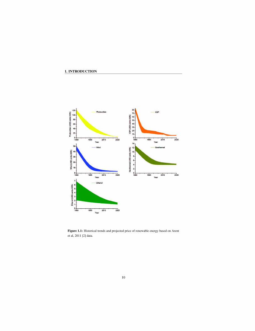
1.1 Historical trends and projected price of renewable energy based on
Arent et al, 2011 [2] data. . . . . . . . . . . . . . . . . . . . . . . 10
1.2 Environmental Kuznets Curve. . . . . . . . . . . . . . . . . . . . 31
2.1 Left: Evolution of population in Ecuador 1980-2010. Right: Growth
rate. . . . . . . . . . . . . . . . . . . . . . . . . . . . . . . . . . 46
2.2 Left: Evolution of GDP and GDP per capita in Ecuador 1980-2010.
Right: Growth rate. . . . . . . . . . . . . . . . . . . . . . . . . . 47
2.3 Productive Sector Matrix in Ecuador 1980-2010. . . . . . . . . . 49
2.4 Top: Evolution of income by productive sector in Ecuador 1980-
2010. Bottom: Growth rate. . . . . . . . . . . . . . . . . . . . . . 50
2.5 Left: Evolution of primary energy consumption and energy intens-
ity in Ecuador 1980-2010. Right: Growth rate. BUSD corresponds
to billion USD. . . . . . . . . . . . . . . . . . . . . . . . . . . . 51
2.6 Evolution of Energy Matrix by productive sectors in Ecuador 1980-
2010. . . . . . . . . . . . . . . . . . . . . . . . . . . . . . . . . 53
2.7 Top: Evolution of energy use by productive sectors in Ecuador
1980-2010. Bottom: Growth rate. . . . . . . . . . . . . . . . . . 54
2.8 Top: Evolution of energy intensity by productive sectors in Ecuador
1980-2010. Bottom: Growth rate. . . . . . . . . . . . . . . . . . 55
2.9 Evolution of Energy Matrix by energy source in Ecuador 1980-2010. 56
2.10 Evolution of Fuel Matrix by source in Ecuador 1980-2010. . . . . 57
xv

LIST OF FIGURES
2.11 Evolution of Fuel consumption by productive sectors in Ecuador
1980-2010. Top: Liquid fuel consumption. Down: Gaseous fuel
consumption. Note that there is not consumption of solid fuel in
the country. . . . . . . . . . . . . . . . . . . . . . . . . . . . . . 58
2.12 Left: Evolution of CO2 emissions and CO2 intensity in Ecuador
1980-2010. Right: Growth rate. . . . . . . . . . . . . . . . . . . 59
2.13 Top: Evolution of CO2 emissions by productive sectors in Ecuador
1980-2010. Bottom: Growth rate. . . . . . . . . . . . . . . . . . 60
2.14 Top: Evolution of CO2 intensity in Ecuador 1980-2010. Bottom:
Growth rate. . . . . . . . . . . . . . . . . . . . . . . . . . . . . . 61
2.15 Top: Evolution of CO2 emissions by fuel in Ecuador 1980-2010.
Bottom: Growth rate. Note that there is not consumption of solid
fuel in the country. . . . . . . . . . . . . . . . . . . . . . . . . . 62
2.16 International average cost range versus preference prices for renew-
able energy in Ecuador based on (Conelec 2009) [3] and (Bruckner
et al 2011) [4]. . . . . . . . . . . . . . . . . . . . . . . . . . . . . 68
3.1 Schematic diagram of the methodology used to build the model. . 74
3.2 Conceptual framework of GDP constitution in Chien and Hu (2008)
[5] . . . . . . . . . . . . . . . . . . . . . . . . . . . . . . . . . . 79
3.3 Conceptual framework of the influences of renewables on GDP in
Chien and Hu (2008) [5] . . . . . . . . . . . . . . . . . . . . . . 80
3.4 SEM model in Chien and Hu (2008) [5] . . . . . . . . . . . . . . 83
3.5 Default CO2 emission factors for combustion - Table 1.4 in IPCC
Guidelines for National Greenhouse Gas Inventories (2006), Volume
2: Energy [6]. . . . . . . . . . . . . . . . . . . . . . . . . . . . . 87
3.6 Default values of carbon content - Table 1.3 in IPCC Guidelines for
National Greenhouse Gas Inventories (2006), Volume 2: Energy [6]. 89
3.7 Default values of carbon content - Table 1.3 (Continued) in IPCC
Guidelines for National Greenhouse Gas Inventories (2006), Volume
2: Energy [6]. . . . . . . . . . . . . . . . . . . . . . . . . . . . . 90
xvi

LIST OF FIGURES
3.8 Causal diagram for the model. Continuous lines stand for the re-
lationship between variables, while dashed ones correspond to con-
trol terms (S:productive sectoral structure, M: energy matrix, U:emission
factors). Bold line represents a feedback mechanism. . . . . . . . 92
3.9 Left: Comparative of model result vs. historical data. Right: Time
series of MAPE term at time t, see Ecuation 3.17. . . . . . . . . . 93
3.10 Left: Estimation of GDP and GDP per capita for the period 2011-
2025 in Ecuador. Right: Growth rate. . . . . . . . . . . . . . . . 98
3.11 Left: Estimation of GDP by sector for the period 2011-2025 in
Ecuador. Right: Growth rate. . . . . . . . . . . . . . . . . . . . . 100
3.12 Estimation of Productive Sectorial Matrix in Ecuador 2011-2025. . 101
3.13 Lefth: Estimation of energy consumption and energy intensity for
the period 2011-2020 in Ecuador. Right: Growth rate. . . . . . . . 102
3.14 Left: Estimation of energy intensity in each productive sector for
the period 2011-2025 in Ecuador. Right: Growth rate. . . . . . . . 103
3.15 Left: Estimation of energy consumption in each productive sector
for the period 2011-2025 in Ecuador. Right: Growth rate. . . . . . 104
3.16 Estimation of energy matrix for the period 2011-2025 in Ecuador. 105
3.17 Left: Estimation of CO2 and CO2 intensity for the period 2011-
2025 in Ecuador. Right: Growth rate. . . . . . . . . . . . . . . . 106
3.18 Left: Estimation of CO2 intensity in each productive sector for the
period 2011-2025 in Ecuador. Right: Growth rate. . . . . . . . . . 107
3.19 Left: Estimation of CO2 in each productive sector for the period
2011-2025 in Ecuador. Right: Growth rate. . . . . . . . . . . . . 108
4.1 Bar view of the CO2 emission additive decomposition factors for
the period 1980-2025 in Ecuador. . . . . . . . . . . . . . . . . . . 129
4.2 View of the CO2 emission multiplicative decomposition factors for
the period 1980-2025 in Ecuador. . . . . . . . . . . . . . . . . . . 131
4.3 Pictorial view of the CO2 emission multiplicative decomposition
factors for the period 1980-2025 in Ecuador. . . . . . . . . . . . . 132
4.4 Dtot/Dact for the period 2011-2025 in Ecuador. . . . . . . . . . . 133
xvii
LIST OF FIGURES
5.1 Different effects of income on environmental degradation as presen-
ted in Islam et al. (1999) [7] . . . . . . . . . . . . . . . . . . . . 137
5.2 Schematic plot of the relationship between the per capita income
and the CO2 emission: 1) linear growth of the pollution with the
GDP, 2) stabilization, and 3) reduction of the emissions with the
increase of the income. Figure adapted from Iglesias et al. (2013)
[8]. . . . . . . . . . . . . . . . . . . . . . . . . . . . . . . . . . . 144
5.3 Top: Estimation of GDP per capita for the period 2011-2025 in
Ecuador. Bottom: Estimation of CO2 emission per capita for the
period 2011-2025 in Ecuador. . . . . . . . . . . . . . . . . . . . 146
5.4 GDP per capita versus CO2 emission per capita for the period 2011-
2025 in Ecuador. Marks TP-ST1-ST2 stand for the year of the
turning points (the scenario passes from stage 1 to state 2) of the
EKC (see Figure 5.5). . . . . . . . . . . . . . . . . . . . . . . . 147
5.5 Evolution of CO2-GDP elasticity for the period 2010-2025 in Ecuador.
150
xviii
List of Tables
3.1 Summary of descriptive statistics for the economic model. . . . . 81
3.2 Estimated coefficients for the GDP formation equations (see Eqs.
3.3-3.7)a. . . . . . . . . . . . . . . . . . . . . . . . . . . . . . . 84
3.3 Mean absolute percentage error (MAPE) for selected variables. . . 94
4.1 Aggregate data for Ecuador for the period 1980-2025. . . . . . . . 128
4.2 Results of the CO2 emission additive decomposition factors for the
period 1980-2025. . . . . . . . . . . . . . . . . . . . . . . . . . . 128
4.3 Results of the CO2 emission multiplicative decomposition factors
for the period 1980-2025. . . . . . . . . . . . . . . . . . . . . . . 130
5.1 Ng-Perron unit root test. . . . . . . . . . . . . . . . . . . . . . . 149
5.2 Stock -Watson-Shin’s DOLS a,b,c,d estimation of linear cointegration.151
xix

ACRONYMS
• ADF Augmented Dickey-Fuller
• AGE Applied General Equilibrium
• AR Auto-Regression
• BAU Business As Usual
• bbl Oil Barrel
• BEC Banco Central del Ecuador, Ecuadorian Central Bank
• BUSD Billion United State Dollar
• CGE Computable General Equilibrium
• CO Carbon Monoxide
• COE Compensation of Employees
• CSP Concentrated Solar Power
• DA Decomposition Analysis
• EEA European Environment Agency
• EFOM Energy Flow Optimization Model
• EKC Environmental Kuznets Curve
• EU European Union
• FDI Foreign Direct Investment
• FTP Feed-in Tariff Policies
• gCO2e Grams of Carbon Dioxide Equivalent
• GDI Gross Domestic Income
• GDP Gross Domestic Product
• GED Global Environmental Degradation
xx

ACRONYMS
• GIGO Garbage Input Garbage Output
• GLS Generalized Least Squares
• GMI Gross Mixed Income
• GNP Gross National Product
• GOS Gross Operating Surplus
• GHG Greenhouse Gas Gases
• HDI Human Development Index
• HP Hodrick and Prescott
• ICTs Information and Communication Technologies
• IDA Index Decomposition Analysis
• IEA International Energy Agency
• IPAT Human Impact, Population, Affluence, Technology
• IPCC Intergovernmental Panel on Climate Change
• ISIC International Standard Industrial Classification of All Economic Activities
• kWh kilowatt hour
• LPG Liquefied Petroleum Gas
• LEAP Long range Energy Alternatives Planning
• LMDI Logarithmic mean Divisia index
• MA Moving Average
• MAPE Mean Absolute Percentage Error
• MB Marginal Benefit
• MC Marginal Cost
xxi
ACRONYMS
• MARKAL Market Allocation
• MEDEE Model for Long-Term Energy Demand Evaluation
• NAFTA North American Free Trade Agreement
• NOx Nitrogen Oxides
• PP Phillip-Perron
• PPP Purchasing power parity
• PSM Productive Sectors Matrix
• PV Photovoltaics
• REN21 Renewable Energy Policy for the 21st Century
• RGSR Renewables Global Status Report
• RPS Renewable Portfolio Standards
• SD System Dynamics
• SDA Structural Decomposition Analysis
• SEM Structural Equation Modeling
• SP&M Subsidies on Production and Imports
• SOx Sulfur Oxides
• SRRES Special Report on Renewable Energy Sources
• SUR Seemingly Unrelated Regression
• TB Trade Balance
• TP&M Taxes on Production and Import
• UK United Kingdom
• US United States
xxii
ACRONYMS
• USD United States Dollar-2005-PPP
• WB World Bank
• WEC World Energy Council
xxiii


The beginning is the most important
part of the work.
Plato
CHAPTER
1Introduction
1.1 The challenges of sustainable development and en-
ergy
Climate change, energy and sustainable development is nowadays a key issue in
the global scientific and political agendas. These issues have important implica-
tions for the development process and national policy in all regions of the planet.
Through Kyoto Protocol, most industrialized nations have committed to reduce
their emissions. In particular, The climate and energy package in European Union
(EU) which is a set of binding legislation aims to ensure that the region meets its
ambitious climate and energy targets for 20201 [9] and most recently, in May 2014,
the United States (U.S.) Global Change Research Program released the Third Na-
tional Climate Assessment (Melillo, 2014) [10], the authoritative and comprehens-
ive report on climate change and its impacts in U.S. where Obama’s administration
showed its concern on climate change and on its effects.
1These targets, known as the ”20-20-20” targets, set three key objectives for 2020:
i) A 20% reduction in EU greenhouse gas (GHG) emissions from 1990 levels;
ii) Raising the share of EU energy consumption produced from renewable resources to 20%;
iii) A 20% improvement in the EU’s energy efficiency [9].
1

1. INTRODUCTION
Political debates and policy decisions with respect to energy and emissions in-
volve a wide spectrum of fields and competences. National planning and policy
processes, including: national development policy, sustainable development, envir-
onment, energy, climate and technology in fields such as spatial development, eco-
nomic development, societal well-being and public education are relevant. Many
of this spheres require an enhancement of its knowledge.
The United Nations Conference on Environment and Development, also known
as the Earth Summits held in Stockholm (Sweden) in 1972, Rio de Janeiro (Brazil)
in 1992 and Johannesburg (South Africa) in September 2002. In 2012, the United
Nations Conference on Sustainable Development was also held in Rio (commonly
called Rio+20 or Rio Earth Summit 2012). These meetings had a very outstanding
outcome and guidance on arrangements for the signatory states in activities related
with the environment.
The Rio Declaration on Environment and Development 1992 (UN, 1992) [11]
establish that: Human beings are at the centre of concerns for sustainable develop-
ment (Principle 1). States have the sovereign right to exploit their own resources
pursuant to their own environmental and developmental policies, and the respons-
ibility to ensure that activities within their jurisdiction or control do not cause
damage to the environment of other States or of areas beyond the limits of national
jurisdiction (Principle 2). In order to achieve sustainable development, environ-
mental protection shall constitute an integral part of the development process and
cannot be considered in isolation from it (Principle 4). To achieve sustainable de-
velopment and a higher quality of life for all people, States should reduce and
eliminate unsustainable patterns of production and consumption and promote ap-
propriate demographic policies (Principle 8). States shall facilitate and encourage
public awareness and participation by making information widely available (Prin-
ciple 10). States shall enact effective environmental legislation (Principle 11). En-
vironmental impact assessment, as a national instrument, shall be undertaken by
States (Principle 17) and that indigenous people, their communities and other local
communities, have a vital role in environmental management and development be-
cause of their knowledge and traditional practices. States should recognize and
duly support their identity, culture and interests and enable their effective particip-
ation in the achievement of sustainable development (Principle 22).
2
1.1 The challenges of sustainable development and energy
On the other hand, one of the most interesting definitions of Sustainable De-
velopment refers to the development that meets the needs of the present without
compromising the ability of future generations to meet their own needs (Principle
3).
A key factor of economic development in countries and the transition from sub-
sistence agricultural economies to modern industrial societies which are oriented
to services, is to have an adequate supply of affordable energy. Energy is essential
to enhance the social and economic welfare and, in most cases, it is essential to
attract industrial and commercial wealth. It is a condition, sine qua non. to support
poverty alleviation, generalize social protection and raise living standards. Note
that no matter how essential energy1 can be for the development, energy is just a
medium, it is not the final goal, while the final goal of sustainable development is
to achieve good health, a high standard of living, sustainable energy and a clean
environment.
As already mentioned, energy consumption is one of the greatest measures of
progress and well-being of a society. The concept of energy crisis appears when
the energy sources of the society are depleted. An economic model as the present,
whose operation depends on continued growth, also requires an equally growing
demand for energy. Since fossil energy sources are finite, it is inevitable that at
some point the demand can not be supplied and all the system will collapse unless
new sources of energy would be discovered or new techniques are developed, as
would be the case of renewable energy.
The energy obtained from virtually inexhaustible natural sources is called re-
newable energy, because this kind of sources contain a vast amount of energy, and
also they are able to be regenerated by natural means in relatively short times.
The potential of renewable energy has a great capacity to help meet global
energy demand. Furthermore, this type of clean energy has a rapid growth due
to the remarkable technical advances that have taken place in recent years and of
society.
1 It is worthy to note that there are no form of energy: coal, solar, nuclear, wind or any other
type, that is inherently good or bad, and each is valid only to the extent that meets the purpose for
which it was created.
3

1. INTRODUCTION
The commitment to promote this type of development and the rational use of
energy, involves setting goals at national and regional levels and define a policy
according with these goals.
1.2 Trends in technology of renewable energy
Climate change, peak oil and energy security are the trends that are setting the pace
of the global energy transition. New types of technologies are required to supply
the growing energy demand and thus stop the historical dependence on fossil fuels.
Faced with this challenge, the technologies related to renewable energy are receiv-
ing strong incentives and stimuli, leading to a global development. Some of these
technologies has become competitive alternatives to traditional energy generation
and start having a display and commercial use.
Indeed, the last three decades of investment in renewable energy sources have
allowed cost reductions close to 40% in technologies related to biomass, 70% in
geothermal and 90% in wind, solar photovoltaic and solar thermal (Arent et at.
2011) [2]. Therefore, it is important to interpret the state of the global trends in
development and dissemination of technologies of renewable energy.
This section is intended to show the level of technological development of the
main renewable energy technologies. Note that these technologies should be in an
advanced stage of its development (deployment and marketing) to have the poten-
tial to be used in developing countries such as Ecuador.
1.2.1 Wind energy
Wind power is one of the more mature renewable energy sources in the world and
the fastest growing in the last three decades (IEA, 2011a [12], WEC, 2010 [13]).
This development has focused on wind turbines on land (onshore) with the three-
bladed rotors model. The overall trend of the average cost 1 of wind power shows
a marked reduction in the last years and in 2025 is projected to be less than 5
1Average costs refer to the total incurred for the operation of a power plant. These include
the costs of investment, operation, maintenance and financing. They are expressed in terms of the
energy produced by the power plant during its life cycle (e.g. US/kWh) (Wiser et al, 2011) [14].
4
1.2 Trends in technology of renewable energy
USD-cents/kWh (see Figure 1.1) (Arent et al., 2011) [2]. Although wind energy is
a technology already being marketed and widespread disseminated, it is expected
that there would be incremental advances and improvements in its design, more
efficient use of materials, reliability and energy capture, reduction of operating and
maintenance costs and longer life of the components.
Technological advances may lead to further cost reductions, facilitating its de-
ployment and adoption in developing countries. Wind power prices are competitive
compared to traditional energy systems based on fossil fuel. (Wiser et al, 2011 [14];
Arent et al. 2011 [2]). It is estimated that the average cost of onshore turbine tech-
nologies will be reduced between 10% and 30% for 2020 and ranges between 15%
and 35% by 2030, regardless of cost reductions and incentive policies to facilitate
the adoption of these systems (e.g. feed in tariff-FIT 1) (Wiser et al., 2011) [14].
The technological development of other kind of wind energy such as wind tur-
bines (offshore) and even floating turbines at sea are already a reality in developed
countries (especially in Europe) (Wiser et al., 2011) [14]. The costs of these tech-
nologies are still higher than onshore turbines, since this kind of technology have
a lower level of overall development. However, future reductions are also expected
in the average costs of these technologies, ranging between 10% and 40% by 2020
and 20% to 45% by 2030 (Wiser et al., 2011) [14].
1.2.2 Solar energy
There is a wide range of solar energy technologies for use in heating, lighting,
electricity, among others. These technologies have varying degrees of maturity and
development. Since the 2000s the fastest growing of renewable energy are solar
photovoltaic modules (Arvizu et al., 2011) [16].
Among solar technologies, the most competitive prices compared to traditional
energy sources are solar thermal systems for heating and water heating. Others
whit are at the stage of deployment and use, at an increasing rate, are photovoltaic
(PV) systems for electricity generation. Most installations of photovoltaic systems
1FIT is a policy mechanism designed to accelerate investment in renewable energy technolo-
gies. It achieves this by offering long-term contracts to renewable energy producers, typically based
on the cost of generation of each technology (Couture, 2011) [15].
5
1. INTRODUCTION
correspond to panels on roofs of houses and, connected to the grid of the city (Ar-
vizu et al., 2011) [16]. Note that a trend of decentralized solar energy systems is
also starting to be developed.
Other technological options are developing solar power generation systems
based on concentrated solar power (CSP) used in some power plants. Designs in-
clude dyes sensitized to capture solar energy and solar cells from organic materials.
Also, they are developing solar technologies for producing fuels such as hydrogen
or hydrocarbons and to store a greater amount of energy in efficient carriers (Arvizu
et al., 2011) [16].
Advances in solar thermal technologies for heating show developments en-
abling longer life of the systems, lower installation costs and higher temperatures.
The trend is that these systems may be essential components of all the roofs of
houses and buildings. In addition, recent designs in storage and conversion of heat
and cold allow use the walls of buildings as active systems of air conditioning and
heating (Arvizu et al., 2011) [16].
In PV panel technologies, future developments aimed at improving the per-
formance (efficiency) and environmental and sustainability profiles in the manu-
facture of the modules. Advances aim to improve not only the panel that captures
energy but the entire system (power inverter, battery, control and network) to con-
vert that energy into electricity according to the standards used in end use appli-
ances in houses.
The technological evolution during last four decades in solar energy has al-
lowed a cost reductions of nearly 80% in PV systems. Indeed, since the PV systems
reach further deployment in the market, their costs are projected to continue to de-
cline rapidly. Based on these trends of technological development and the increase
in the world market, it is projected the average cost of PV systems to be reduced by
more than 50% and may reach an average of 7.3 USD-cents/kWh in 2020 (Arvizu
et al., 2011) [16].
1.2.3 Bioenergy
Bioenergy production is an option to diversify the energy sources in the world
(Kammen, 2004) [17] due to its large energy efficiency, clean and cost-competitive.
6

1.2 Trends in technology of renewable energy
Commercial available technologies are: heating and electricity generation through
combustion of biofuels. Biofuels come from oil crops, such as biodiesel, and sugars
and starches, such as ethanol (Chum et al., 2011) [18].
There are also small-scale systems that use bioenergy to provide heat for cook-
ing, anaerobic digestion systems for treating solid waste and produce methane gas
for burning (heating, cooking) and gasifiers.
These technologies use a wide range of agricultural products. Most existing
bioenergy systems are mainly based on wood and agricultural residues for the pro-
duction of heat and electricity, and agricultural crops for the production of liquid
biofuels. The energy performance of these systems vary due to the conversion
technology and material used (crop residues, pulp). Charcoal is one of the most
frequent uses of bioenergy in developing countries, especially in rural areas, how-
ever, production can be improved with cleaner and more efficient furnaces (Chum
et al., 2011) [18].
Another technology still in development status and still holding high costs is
second-generation biofuel. These are manufactured from non-food biomass which
crops require less both water and land for its production, or from agricultural and
forest residues. It is under investigation and in its early stages of production, bio-
fuels based inedible lignocellulosic biomass, including crop residues and wood
production (such as rice husk, corn husk or sawdust), inedible plant crops in which
whole plant is used (such as switchgrass) and vegetable oils crops that do not com-
pete for land use (such as biodiesel from microalgae) (Carriquiri et al., 2011) [19].
Biomass is the only renewable energy where can be obtained liquid high energy
density fuels to replace fossil fuels in transport by land, air and maritime (Chum et
al., 2011) [18].
Trends in bioenergy costs are varied and depend on the prices of agricultural
raw materials and on applied technology for conversion and energy use. Hence,
the main factors affecting costs are the costs of bioenergy crop production, trans-
portation to processing centers (these two may represent between 20% and 50% of
the total average cost) and technical specificities the used technology (Chum et al.
2011) [18].
The cost projections for bioenergy are subject of uncertainty. However, based
on the trends of improvement and maturity of the technology, can be estimated a
7
1. INTRODUCTION
cost reduction close to 40% for the production of ethanol from sugarcane in coun-
tries like Brazil and 20% for corn ethanol in U.S. by 2020. Second-generation
biofuels based on lignocellulosic materials also have the potential to reduce its cost
production in medium term, which could compete with the prices of gasoline and
diesel from a barrel of oil at USD 60- 70/bbl1 (0.38 to 0.44 USD per liter of ethanol)
by 2030 (Chum et al., 2011) [18].
1.2.4 Wave and tidal energy
This type of technology is still at an embryonic stage and is not commercially
available yet. The industry dedicated to the development of this technology is
focused in the design and evaluation of prototypes for harnessing wave and tidal
energy (REN 21, 2011 [20] and Lewis et al, 2011 [21]). The only exception is the
use of tidal energy through dams, similar to hydroelectric dams design, located in
the sea estuaries (Lewis et al., 2011) [21].
Prototypes so far do not converge to a unique design as in the case of wind
turbines where the consensus has resulted in a three-bladed model. Due to this
fact, there are several options for energy use and a unique design is not likely in
this technology. The investment cost and the average cost of electric generation is
not yet competitive (between 12 and 22 USD/ kWh) compared to other renewable
energy sources, even worse when compared with traditional sources (Lewis et al.,
2011) [21].
1.2.5 Geothermal energy
Geothermal is one of the most promising alternatives for energy supply in the long
term. A technological option is the use of high temperature fluids to generate elec-
tricity through turbines. To this end, there are two alternatives: use the natural
hot spring pools or enhanced geothermal systems with the use of artificial fluids
(Goldstein et al, 2011) [22].
1An oil barrel (abbreviated as bbl) is a unit of volume whose definition has not been universally
standardized. In the U.S. and Canada, an oil barrel is defined as 42 U.S. gallons, which is about 159
liters or 35 imperial gallons, and it can also be defined in those units, depending on the context.
8

1.3 Integration of renewable energies in energy systems
Thermal water reservoir is a mature and reliable technology (it has over 100
years of operation). Enhanced geothermal systems are still in demonstration phase.
Geothermal energy has a great potential to generate electricity due to the high levels
of efficiency that can be achieved (load factor1). This feature is an advantage over
other renewables such as solar, wind and hydroelectric, because these technologies,
by their variable and intermittent nature, have a fickle electricity production based
on the availability of the source that use. Indeed, the global average load factor
of geothermal systems for power generation is 74.5%. The new geothermal plants
reach higher ground factors 90% (Goldstein et al., 2011) [22].
The power plants based on geothermal reservoirs of hot springs have high ini-
tial investment costs, because it is necessary to explore and drill similarly to those
of the oil industry wells. However, operating costs are low and do not use fuels.
Therefore, the average cost of electricity from these systems is competitive. De-
pending on the level of utilization of the resource, the range is between 0.03 and
0.17 USD/kWh. The cost of enhanced geothermal systems is still greater than this
traditional source (Goldstein et al., 2011) [22].
Technological advances point to improve the reliability and energy recovery
as well as increase the life cycle of plants. Therefore, research and development in
the exploration of hidden geothermal resources is required. This type of geothermal
resource is characterized by not showing water reservoirs, so they are exploited by
improved systems. As a result of technological improvements, it is expected that
the average cost of generation from geothermal water reservoirs decrease by 7% in
2020 (Goldstein et al., 2011) [22].
1.3 Integration of renewable energies in energy sys-
tems
The analysis of the potential of renewable energy for changing the energy matrix
is done on the basis of treating them as energy systems rather than from the per-
spective of technical and economic parameters of each technology (Kriegler, 2011)
1In electrical engineering the load factor is defined as the average load divided by the peak load
in a specified time period.
9
1. INTRODUCTION
Figure 1.1: Historical trends and projected price of renewable energy based on Arent
et al, 2011 [2] data.
10

1.3 Integration of renewable energies in energy systems
[23].
In order to minimize the risks inside an energy system and to have greater reli-
ability in the provision of energy is needed: diversification of energy sources, flex-
ibility and complementarity between adopted technologies, extent of energy infra-
structure (interconnection, transmission and distribution), the use of energy storage
technologies and mainly of institutional and market mechanisms to improve secur-
ity and energy supply (Sims et al., 2011) [24]. It is needed well-diversified energy
sources to face the challenge of replacing fossil fuels as a primary energy source
worldwide, in Latin America and in Ecuador.
According to IPCC (2011) [25], in the best case, about 77% of the world energy
matrix can be supplied from the use of renewable resources. Some countries are
exploring the possibility of having an energy matrix based 100% on renewable
energy sources. Such is the case in Denmark, where by 2030 is aiming to achieve
50% and 100% by 2050. The energy matrix of each country should be based on
the resources with the greatest potential in each nation (Lund and Mathiesen, 2009)
[26].
Planning for an energy system based 100% on renewable energy sources is
physically possible in allocation terms of energy resources. Some authors describe
three scenarios regarding the reorganization of the energy systems around the re-
placement of fossil fuels worldwide. The first is the extensive use of bioenergy
to supply the non-electric energy demand (e.g., transportation fuels), in particular
the use of biofuels. In this scenario, the biggest challenge is how to organize a
sustainable coexistence between agriculture for food, conservation of ecosystems
and bioenergy production. The second generation biofuels can make a significant
contribution in reducing pressure, using waste water and marginal land, but their
development still requires competitive costs (Kriegler, 2011) [23].
The second scenario suggests the production of fuels and energy storage with
renewable technologies (other than biomass) . The limitations of renewable energy
sources, e.g., intermittency, geographic dispersion and electrical use are removed
when used for the production of fuels such as hydrogen. The challenges for this
scenario are the massive changes in energy infrastructure in order to use hydrogen
at large-scale. However, there are criticisms about cost and efficiency of hydrogen
11

1. INTRODUCTION
as fuel and energy storage, but certainly this type of energy can be transported to
end-uses (e.g., fuel cells in cars) (Kriegler, 2011) [23].
The third scenario considers electrify transport and heating. This scenario re-
quires technologies such as hybrid electric vehicles (plug in), among others, and
may be feasible since there is already infrastructure to provide electric energy to
end users. Extra advantage is the high efficiency of electric engines. However,
it is required to improve battery technology for electric vehicles and the electric
transmission grid to incorporate decentralized generation (Kriegler, 2011) [23].
Another challenge is to incorporate decentralized generation systems to the en-
ergy matrix. Traditionally, electrical systems were designed to transport energy
from large scale power plants (hydroelectric, thermoelectric and nuclear) with high
voltages to local distribution networks, with lower voltages. However, due to the
disperse distribution of renewable energy sources, energy transition to a greener
matrices requires that the grid transmission manage several medium and small gen-
erators connected to distribution systems (Bayod-Rujula, 2009) [27].
With the increasing demand of energy and the necessity of decarbonised en-
ergy systems, the world is beginning to understand that diversified and decent-
ralized systems make a energy matrix more robust. This robustness has several
advantages: lower concentration in few sources, lower risk of natural disasters and
climate change effects and greater diversification of energy sources (Ebinger and
Vergara, 2011 [28]; Bouffard and Kirschen, 2008 [29]; Nair and Zhang, 2009 [30]).
Decentralized energy systems involves challenges for transmission infrastruc-
ture. The management of electricity distribution networks by information, commu-
nication and control infrastructure is required, in order to manage the increasing
complexity of having several generators connected to the system. In this sense,
there are new concepts and perspectives as micro grids, virtual power plants (Bayod-
Rujula, 2009) [27] and smart grid (Lindley, 2010) [31].
Smart grid is a concept that involves electrical transmission systems that incor-
porate the new information and communication technologies (ICTs) with transmis-
sion lines and distribution channels (Nair and Zhang, 2009) [30]. The purpose of
smart grids is to optimize the operation of the electricity market and create a reli-
able and affordable transmission. This system would allows multiple options for
managing electricity demand in order to reduce the peaks, to have greater efficiency
12
1.4 Methodological issues and exploration of future changes
and to interconnect between communities and households to exchange information
and energy flows (Lindley, 2010) [31].
1.4 Methodological issues and exploration of future
changes
The understanding of future changes in energy and emissions for both policy and
reporting in the areas under study start from official data sources such as the World
Bank, the International Energy Agency, Central Banks and Institutes of Statistics
and Census of a given country or region. To carry out projections of energy use
and emissions can be problematic, due to inertia in infrastructure, technology and
even culture of each country or region. Note that short term decisions can have
long term consequences. They can embed a long term development path that limits
or prevents emission reductions and hence an environmental protection. According
to Van’t Klooster and Van Asselt (2006) [32], studies on the future of a system is
complex, as many relations that may seem to have been continuously developed in
retrospect, often follow a non-linear model in future. Those authors propose that it
may be legitimate to hold different and often conflicting perspectives on how the
future can reveal. Armstrong (2001) [33] discusses two key sources of uncertainty
in forecasting in general. These are overconfidence in forecast due to uncertainty in
the causal variables in an econometric model and assumptions about relationships
that may not hold over the forecast horizon. Agnolucci et al. (2009) [34] suggest
that the past is not necessarily a good guide to the future in the context of energy
and emissions. The predictability of energy and emissions and the accuracy of the
predictions have been questioned even in the short term.
It is often not possible to make an assessment and ex-post forecast on energy
or emissions with high accuracy. Linderoth (2002) [35] among others, described
large forecast errors in determining future energy consumption in countries mem-
ber of IEA. These sometimes conceal the sum of considerable positive and negative
forecast errors in the sectors, particularly in industry and transport. This author in-
dicates that the underestimate of transport can have particular consequences for
emission reduction policy. Winebrake and Sakva (2005) [36] found a low mean
13
1. INTRODUCTION
percentage error for total energy consumption concealing an average 5.9% over-
estimate for the industry sector and 4.5% underestimate for the transport sector in
U.S.. O’Neill and Desai (2005) [37] noted that the errors occur not only in abso-
lute values and sectoral consumption, but in GDP growth rates, energy intensity
improvement and in fuel mix. This reduces the potential accuracy of forecast of
GHG emissions and, as they are an input into policy processes, has potential fur-
ther consequences. Errors can occur even on short time-scales. Linderoth (2002)
[35] concluded that large forecast error can occur even when the forecast year is
close to the review year.
Pilavachi et al. (2008) [38] state that the Energy 2000 study of the European
Community in 1985 underestimated consumptions of oil and gas and overestim-
ated solid fuels and renewable energy in 2000 of most of the EU countries. The
author found a substantial forecast error over the EU and outlined three areas of
uncertainty: i) unanticipated strong political decisions, ii) unanticipated energy
requirements and iii) data definition and availability. In this context, the potential
significance of such overestimations/underestimations is not just in meeting targets
in environmental protection but also in cost effectiveness and cost benefit analysis
of measures to meet targets.
On the short and medium term there is a clear benefit in using sectorally dis-
aggregated scenarios. These can show variation in absolute totals of energy con-
sumption and emissions. They can also illustrate potential divergent trends in, for
example, sectoral contribution, economic growth rates and energy intensity change.
de Jouvenel (2000) [39] stated that simulation models based on observations of the
past are favoured by economists, econometrists, statisticians and forecasters. In
addition, the accuracy or scientific quality of forecasts is not guaranteed where res-
ults may be arbitrary and subjective because can be subject to the GIGO effect
(Garbage In Garbage Out). This method has long been opposed to the scenario
method, which is more developed and used by futurists for one simple reason: bet-
ter a rough but fair estimations than a refined yet incorrect forecast (de Jouvenel,
2000) [39]. In addition, technological and economic realities are implicitly embed-
ded in energy modelling apparatus while results are often promoted as objective
(Nielsen and Karlsson, 2007) [40]. Middtun and Baumgartner (1986) [41] termed
14
1.5 Data sources and data pre-processing
this combination of modelling and politics as the scientific negotiation of energy fu-
tures. It increases the need for not only reproducible results and published models,
but transparent assumptions and dynamics in studies related to energy and emis-
sions modelling.
Note that, even in a short period, uncertainty in emissions projections can arise.
This uncertainty is a challenge to probabilistic and predictive methodologies and
suggests that scenarios are useful to delimit uncertainty. While forecasts are use-
ful, it can also give an illusion of certainty. The continual revision of the CO2
and energy projections for different countries and regions by the most of authors
illustrates some of the methodological difficulties encountered by forecasting.
1.5 Data sources and data pre-processing
Data sources and statistics collected by an officially recognized national body are
usually the most appropriate and accessible data. In some countries, however, those
charged with the task of compiling inventory information may not have ready ac-
cess to the entire range of data available within their country and may wish to use
data specially provided by their country to the international organizations. In re-
gard to this dissertation two main types of data sources will be distinguished, on
one hand, population and economic activity and on the other, energy and fuels.
1.5.1 Population and economic activity data
Currently, there are two main international sources about population and economic
activity statistics: the World Bank (WB), and the International Monetary Found
(IMF). Both international organizations collect population and economic statistics
from the national administrations of their member countries through systems of
questionnaires.
In the case of WB, this database presents population and other demographic
estimates and projections from 1960 to 2050. They are disaggregated by age-group
and gender and cover approximately 200 economies.
Economic data here covers measures of economic growth, such as gross do-
mestic product (GDP) and gross national income (GNI). It also includes indicat-
15
1. INTRODUCTION
ors representing factors known to be relevant to economic growth, such as capital
stock, employment, investment, savings, consumption, government spending, im-
ports, and exports.
1.5.2 Energy and fuel data
The main international sources related to energy and fuel statistics are: the In-
ternational Energy Agency (IEA), the United Nations (UN) and in particular in
Latin-America the Latin American Energy Organization (OLADE). All this or-
ganizations collect energy data from the national administrations of their member
countries through systems of questionnaires, thus, data gathered are official.
Many countries have long time series about energy statistics that can be used
to derive time series about GHG emissions. However, in many cases statistical
practices (including definitions of fuels, of fuel use by sectors) will have changed
over time and recalculations of the energy data in the latest set of definitions is not
always feasible. In compiling time series about emissions from fuel combustion,
these changes might give rise to time series inconsistencies, which should be dealt
using the methods provided in Time Series Consistency Chapter 5 of Volume 1 of
the 2006 IPCC Guidelines [42].
1.5.3 Data pre-processing
Data pre-processing is an important step in the data analysis and model building.
The phrase GIGO is particularly applicable in these kind projects. Data-gathering
methods are often loosely controlled, resulting in out-of-range values (e.g., neg-
ative values in population data), impossible data combinations (e.g., Sex: Male,
Pregnant: Yes), missing values, etc. Analyzing data that has not been carefully
screened for such problems can produce misleading results. Thus, the representa-
tion and quality of data is first and foremost before running an analysis (Pyle, D.,
1999) [43].
When there is much irrelevant and redundant information present or noisy and
unreliable data, the knowledge discovery during the training phase is more difficult.
Data preparation and filtering steps can take considerable amount of processing
16
1.5 Data sources and data pre-processing
time. Data pre- processing includes cleaning, normalization, transformation, filter-
ing, feature extraction and selection, etc. The product of data pre- processing is the
input to analysis and model building phases. Kotsiantis et al. (2006) [44] present a
well-known algorithm for each step of data pre-processing.
In modelling and forecasting works, to remove the effect of seasonal, cyclical
and irregular components from observed data and work only with the trend part
is important. Therefore, decomposition methods in time series to determine the
trends, are required. The Hodrick- Pescott (HP) filter is a method to extract the
trend component of a time series, proposed in 1980 by Robert J. Hodrick and Ed-
ward C. Prescott (Hodrick and Prescott (1980)) [45]. It decomposes the observed
series into two components: i) the trend component and ii) the cyclical component.
The sensitivity setting of the trend to short-term fluctuations is obtained by modi-
fying a multiplier called λ. It is currently one of the most widely used techniques
in research on business cycles to calculate the trend of the time series, as it gives
more consistent results with the observed data than other methods.
According to Hodrick and Prescott (1980) [45], HP filter has its origin in the
method of Whittaker-Henderson Type A, which was first used by actuaries to smooth
life tables, but also has been useful in studies of astronomy and ballistics. Kydland
and Prescott (1990) justify the use of this filter for its linearity, being well defined
without subjective elements, independent of the series to which it applies and easy
to replicate to find the trend that one could draw freehand (Kydland, E, and Prescott
E, 1990) [46].
The reasoning for the methodology uses ideas related to the decomposition of
time series. Let yt, for t = 1, 2, ..., T , denote the time series variable. The series yt,
is made up of a trend component, denoted by τ , and a cyclical component, denoted
by c, such that yt = τt + ct. Given an adequately chosen, positive value of λ, there
is a trend component that will solve the following equation:
min
(
T∑
t=1
(yt − τt)2 + λ
T−1∑
t=2
[(τt+1 − τt)− (τt − τt−1)]2
)
(1.1)
The first term of Equation 1.1 is the sum of the squared deviations dt = yt − τt
which penalizes the cyclical component. The second term, which is multiple by λ
corresponds to the sum of the squares of the trend component’s second differences.
17

1. INTRODUCTION
This second term penalizes variations in the growth rate of the trend component.
The larger the value of λ, the higher is the penalty. Hodrick and Prescott suggest
1600 as a value of λ for quarterly data under the assumption of disturbances having
effects during at least 8 years or more permanent. For monthly series is usually
used λ = 14400 and for annual series a value of λ = 100 is recommended.
1.6 Decomposition of the driving forces of change
It is well known that humans have dramatically altered the global environment, but
there is a limited understanding of the driving forces of these impacts. The absence
of a refined set of analysis tools is cited as a fundamental limitation (York et al.,
2003) [47]. Analysis methodologies and tools have been developed in the field of
analysis of decomposition, including sustainability framework known as the IPAT1
(Commoner, 1972 [48] and Ehrlich and Holdren, 1972 [49]). The decomposition of
changes in an aggregate environmental impact and of its driving forces has become
popular to unravel the relationship of society and economy with the environment.
The specific application in energy consumption and CO2 emissions is the so
called Kaya identity (Kaya, 1990) [50]. The Kaya identity is a linking expres-
sion of factors that determine the level of human impact on environment, in the
form of CO2 emissions. It states that total emission level can be expressed as the
product of four inputs: population, GDP per capita, energy use per unit of GDP,
carbon emissions per unit of energy consumed. The Kaya identity2 plays a core
role in the development of future emissions scenarios in the IPCC Special Report
on Emissions Scenarios [51]. The scenarios set out a range of assumed conditions
for future development of each of the four inputs. Population growth projections
are available independently from demographic research; GDP per capita trends are
available from economic statistics and econometrics; similarly for energy intensity
1Human Impact (I) on the environment equals the product of P= Population, A= Affluence,
T= Technology. This describes how our growing population, affluence, and technology contribute
toward our environmental impact.2Note that, a limitation of this equation is that it does not account for i) the direct release of
carbon dioxide by deforestation through burning ii) the loss of the carbon sink due to that deforest-
ation.
18
1.6 Decomposition of the driving forces of change
and emission levels. The projected carbon emissions can drive carbon cycle and
climate models to predict future CO2 concentration and climate change.
Some similar conceptual bases can be found in the field of index decomposi-
tion analysis (IDA). In particular, with the advent of the global oil crisis in 1973 and
1974, special attention was given to the use of energy in industry among policy-
makers because energy in industrial constituted most of the primary energy demand
in most countries. Therefore, researchers focused on the mechanisms of change in
industrial energy use. This new area of research emerged to quantify the impact
of a structural change in industrial production on the total energy demand. These
initial studies showed a significant impact of structural changes on the trends of
energy demand. The need to identify and quantify its impact became an imperative
for policy-making. This line of research was expanded considerably in the meth-
odology and in its application, it is now a widely accepted tool for the formulation
of national policies on energy and environment analysis (Ang, 2004) [52]. It is
particularly useful to provide the analysis of contributing factors, such as structural
changes and changes in energy intensity. Steenhof et al., (2006) [53] manifested
that decomposition of a predefined set of factors helps to understand the progres-
sion of the driving forces, the consequences of the processes occurring and the
political dimensions associated with these processes. Steenhof et al., (2006) [53]
also proposed that this would allow a rationalisation for possible progression into
the future.
The scope of the IDA was expanded beyond the analysis of industrial energy
demand, now being used in the analysis, at country level, of fields such as energy
or environment1.
The need for political views 2 of the IDA has mainly focused on historical ana-
lysis of the driving forces. While decomposition techniques such as IPAT can be
used to predict future changes in the driving forces of a given system (Waggoner
and Ausubel, 2002) [54], IDA is on the cusp of a new scenario analysis techniques
1Energy efficiency measures are required by several international and national policies as the
EU directive 2006/32/EC and while these can be executed using tools like IDA and LMDI ( Logar-
ithmic Mean Divisia Index) techniques (Ang, 2004) [52].2The development of policy, reporting and monitoring of progress depends on the right as the
index decomposition analysis analytical tools.
19
1. INTRODUCTION
and forecasting. For defining areas of future research in IDA, Ang and Zhang
(2000) [55] suggests its use in projecting energy demand and emissions in short
and medium term. Sun (2001) [56] used a complete decomposition method to
forecast GHG emissions in the EU-15 up to 2010. Sorrell et al. (2009) [57] re-
commended more research in the use of the decomposition framework for scenario
development. Although both, IDA in energy and emissions, as well as scenario
analysis in the context of energy emissions are often based on the framework of
Kaya, the combination of these approaches has often not applied. In this line some
studies have combined these approaches; Kwon (2005) [58], Steenhof et al. (2006)
[53], Steenhof (2007) [59] and Agnolucci et al. (2009) [34].
Agnolucci et al. (2009) [34] used a retrospective approach to scenarios and
projection ratios decomposition. This approach was used to generate a predefined
result in 2050 to discuss how relationships can be altered to achieve future goals
through public policy. Kwon (2005) [58] used scenario analysis to quantify future
CO2 emissions from car travel in the United Kingdom (UK) until 2030 using the
IPAT framework. This author built a Business as usual (BAU) scenario and al-
ternatives scenarios to make assumptions about the forecast of each of the factors
of the identity used. Steenhof (2007) [59] uses the IDA approach of Laspeyre to
build baselines for the electricity sector in China by 2020. This author uses a BAU,
conservative and optimistic scenarios with the analysis of time series decomposi-
tion (every two years instead of at the beginning and end of year). Steenhof et al.
(2006) [53] also combines the decomposition analysis and the use of scenarios to
project the burden of GHG in the short term (up to 2012) in Canada. Decompos-
ition analysis was performed on the historical pattern to understand impact of the
driving forces, while the scenario analysis provided the means to manipulate these
forces in the future. Again BAU scenarios, optimistic and pessimistic have been
employed.
In the research present in this dissertation about income growth, energy use and
CO2 emissions for Ecuador in medium term (up to 2025), the specific combination
of techniques such as IDA (specifically LMDI approach), the use of exploratory
scenarios and the Kaya identity (Kaya, 1993) [50] is trying to help to fill the gap in
the regional literature in this topic. This study joins the study of the driving forces
of change across both analysis decomposition and scenario analysis.
20
1.7 Background of scenario analysis
1.7 Background of scenario analysis
Scenario analysis has a wide history in a large number of sectors and disciplines
(Van Notten et al, 2003) [60]. It is an approach to deal with uncertainty that may
exist in organizations and governments (Nielsen and Karlsson, 2007) [40]. This
type of analysis has been increasingly applied in the field of energy and environ-
ment, due to difficulties in providing accurate forecasts (Silberglitt et al., 2003)
[61], and to the need for tools to imagining, discuss, and create future scenarios
equally plausible. Specifically in the analysis of environmental settings including
energy and emissions, there are two currents that could be described respectively
as i) inquiry-driven and ii) strategy-driven (Alcamo et al., 2009) [62]. Inquiry-
driven scenario analysis is conducted to meet the needs of the scientific community
through expanding the knowledge and as an input to policy analysis. Strategy-
driven scenario analysis is mainly due to the business community for corporate
planning. The scientific credibility about scenarios theory has been increased due
to the wide spectrum of opportunities for study and analysis that this technique
offered in different fields.
The scenario analysis allows having a structured view of the future of develop-
ment in areas such as driving forces, trends, themes, events and the logic of cause
and effect. The objective of the scenario-based analysis is not prediction, but the
construction and articulation of several different futures and the paths leading to
them (Borjeson et al, 2006) [63]. In particular, climate change depends in part
on the evolution of humans factors such as anthropogenic GHG emissions, popu-
lation, economy, etc. Given the uncertainty of future development, the scenarios
have been used in the Special Report on Emissions Scenarios (SRES) of the Inter-
governmental Panel on Climate Change (IPCC, 2000) [51] as the most suitable tool
for exploring the future evolution of global emissions of GHG by the year 2100.
To study the evolution of complex systems where elements with behaviour not
fully understood exists, the use of scenarios could be compulsory. The scenarios
are not predictions or forecasts, but they are used to explore the equally plausible
images of future developments (Nakicenovic et al, 2000) [64]. Besides, scenarios
have been used as tools to link qualitative and quantitative arguments in modelling.
21

1. INTRODUCTION
The scenarios are also used by intergovernmental bodies such as the IEA and the
European Environment Agency (EEA).
Certain works based on the use of scenarios have tended to focus on the long
term in a world of great uncertainty (Nielsen and Karlsson, 2007) [40]. However, as
indicated above, even in the short and medium-term, the application of the scenario
methodology has scientific credibility and potential usefulness in policy develop-
ment. In this dissertation a set of plausible scenarios for the evolution of CO2
emissions and energy consumption in Ecuador in a medium term (2025) are carry
out. These scenarios explore the evolution of the driving forces, both qualitatively
and quantitatively. The delimitation of uncertainty in response to questions related
to forecast accuracy provides insights into the driving forces of change and explores
the potential contribution of different sectors to the total change of emissions.
1.8 Background of analysis models
The economics and environmental models can be divided in two general groups
according to their structure: i) top-down and ii) bottom-up models (Great Britain.
Department of Energy. Economics and Statistics Division, 1978) [65].
The top-down analysis method is based on a macroeconomic approach and con-
siders the price of the energy and the elasticity as the main economic indicators to
model the relationship between energy consumption and energy production. The
top-down method is mainly applicable to the analysis of macroeconomics and to
research on development of energy policies. However, this approach cannot con-
trol the impact on the economy of advances in technology. Some examples of this
approach are the computable general equilibrium (CGE) model1 based on General
Equilibrium Theory and the Input-Output model.
The bottom-up analysis is a technique to build a model in more detailed way.
Mainly it aims the construction of models of energy consumption and production
for supply-demand forecast and environment impact analysis (Toshihiko, 2004)
[67]. The bottom-up model has two branches in terms of research, which were
1CGE models are a class of economic models that use actual economic data to estimate how an
economy might react to changes in policy, technology or other external factors. CGE models are
also referred to as AGE (applied general equilibrium) models [66].
22
1.8 Background of analysis models
described by Wei (2005) [68]. The first is based on energy supply and conver-
sion, it is frequently used for the analysis of the introduction of efficient techniques
into energy systems and for the analysis on its effects. Typical examples of this
approach are MARKAL model, developed by the IEA and EFOM (Energy Flow
Optimization Model 1) model developed by EU [70]. The second branch analyzes
and calculates in detail the change in energy demand and consumption caused by
the human activities. Representative models are MEDEE (Model for Long-Term
Energy Demand Evaluation) model, developed by France and LEAP (Long range
Energy Alternatives Planning) model, developed by Stockholm Environment Insti-
tute.
Now, we will mention briefly the most relevant models related to energy and
emissions, then we will focus on the approach used in this research, System Dy-
namics (see Section 1.9 in this Chapter).
1.8.1 Input-Output model
Wassily Leontief is credited with developing the Input-Output (I/O model) analysis
[71] and he was awarded the Nobel Prize in Economics in 1973 for his development
of this model [72], which is still considered as one of the most effective theories to
solve the problem of balanced economic growth, as was shown by William (1980)
[73]. This approach could help working out the chessboard type of input-output
statement and setting up the corresponding linear algebraic equation set to form an
economic mathematical model, which could imitate the structure of the actual na-
tional economic system and the social production process, to analyze and confirm,
comprehensively, the complex relationship among all the sectors in the national
economic system and the key production proportional relationship.
1.8.2 LEAP model
LEAP is an integrated modeling tool that can be used to track energy consumption,
production and resource extraction in all sectors of an economy. This model has
1The Energy Flow Optimization Model (EFOM) is the supply part of the energy model complex
of the Commission of the European Communities which has been used for a number of studies
during the last decade [69].
23
1. INTRODUCTION
been developed by the Stockholm Environment Institute and the Tellus Institute
[74]. The model follows the sequence of resource, transition and demand, to assess
the energy demand and supply balance at certain region. This model is used to
design the energy consumption mode in various development scenarios on the base
of the current energy demand of each productive sector. This model also is useful
to perform the forecast of social and economic development in the medium and
long term with different policy packages and techniques selection modes. The
combination of various development modes and their comparison could provide a
reference for decision-making about economic and energy development planning
in a given country or region.
LEAP model is considerate as a terminal energy consumption model. It is
mainly focuses on the achievement of the balance in demand and resource trans-
ition (Joost, 2004) [75]. Moreover, LEAP uses the existing energy technology and
environmental databases to analyze the balance program in terms of cost and pol-
lutant yield. Therefore, LEAP model is suitable to be applied to scenario analysis.
It is possible to set up various policies to draft cases of study and then analyze the
advantages and shortcomings of them.
1.8.3 MARKAL model
In 1976, the IEA developed MARKAL (Market Allocation) model and promoted
many nation initiatives for its use. MARKAL model is an energy system ana-
lysis tool based on multi-objective linear planning method. The model is a partial
equilibrium model mainly composed of an energy database and a linear planning
software. It pays great attention to the energy technologies, it uses 21 kinds of con-
straint equations to assure supply-demand balance and economic growth, and it sets
up an objective function to get an energy program which aim is to get the lowest
cost or the minimum pollutant emission. The model is able to be used for optimiz-
ation and solving, as was shown by Naughten (2003) [76] and Evasio (2004) [77].
1.8.4 SD model
The System Dynamics (SD) is a computer-aided approach to policy analysis and
design developed by J. Forrester at Massachusetts Institute of Technology (MIT) in
24

1.9 The system dynamics approach
1956, applicable to modelling and simulating complex systems. SD allows to study
the cause-and-effect relationship among the factors inside the system and depends
on a computer simulation to conduct a quantitative analysis. SD is characterized
for dependence on the inherent mechanism of a large complex system to complete
the simulation. Thus, once the model is calibrated, it could be used to rightly
forecast the system state. SD is also an approach to understanding the behaviour of
complex systems over time. It deals with internal feedback cycles and time delays
that affect the behaviour of the overall system. What makes different SD from
other approaches, to study complex systems, is the use of feedback-loops, stocks
and flows. These elements, which are described as deceptively simple systems
display a bewildering nonlinearity.
This work tries to model, in macro and sectoral basis, the production system
of a given country and the use of primary energy and fossil fuel. In addition, this
research attempts to use a formation approach of the GDP that includes the effect
of renewable energies, which introduces a feedback mechanism. SD is an ideal
tool to carry out such a task. Therefore, this approach will allow us to draw robust
conclusions about the behavior of the individual components as well as of the whole
system.
1.9 The system dynamics approach
SD is an approach to system theory as a method for understanding the dynamic
behaviour of complex systems. The basis of the method is the recognition that the
structure of any system: the many circular, interlocking, sometimes time-delayed
relationships among its components, is often just as important, in determining its
behaviour, as the individual components themselves. Examples are chaos theory
and social dynamics. It is also claimed that because there are often properties-of-
the-whole which cannot be found among the properties of its elements, in some
cases the behaviour of the whole cannot be explained in terms of the behaviour of
the parts.
SD is currently being used throughout the public and private sector for policy
analysis and design (Radzicki and Taylor, 2008) [78]. The best known SD model
is probably The Limits to Growth (Meadows, Donella H., 1972) [79]. This model
25
1. INTRODUCTION
predicts that exponential growth that would lead to economic collapse during the
21st century under a wide variety of growth scenarios. The use of SD methodology
for the understanding of complex environmental systems has increased signific-
antly in the last decades. SD has been used to study climate change policies and
the evolution of the economy (Naill, 1992 [80]; Nordhaus, 1996 [81]; Fiddman,
2002 [82]; Feng, 2012 [83]). Bassi and Baer (2009) [84] carried out an SD study
trying to answer whether an annual investment of 1% of GDP to mitigate the neg-
ative economic impacts of climate change, would allow for the reduction of GHG
emissions in Ecuador.
SD approach involves, in general, the following aspects:
• Defining problems dynamically, in terms of graphs over time.
• Striving for an endogenous, behavioural view of the significant dynamic of a
system, a focus inward the characteristics of a system that themselves gener-
ates or exacerbates the perceived problem.
• Thinking in all concepts of the real system as continuous quantities intercon-
nected in loops of information feedback and circular causality.
• Identifying independent stocks or accumulations (levels) in the system and
their inflows and outflows (rates).
• Formulating a behavioural model capable of reproducing, by itself, the dy-
namic problem of concern. The model is usually a computer simulation
model expressed in nonlinear equations, but it is occasionally left unquan-
tified as a diagram capturing the stock-and-flow/causal feedback structure of
the system.
• Deriving understandings and applicable policy insights from the resulting
model.
• Implementing changes resulting from model-based understandings and in-
sights.
The theory about SD is extensive, but below we will follow the introduction
given by System Dynamics Society [85]. Further information can be found in
Garcia (2011) [86].
26
1.9 The system dynamics approach
1.9.1 Modelling and simulation
Mathematically, the basic structure of a formal SD computer simulation model is a
system of coupled, nonlinear, first-order differential (or integral) equations,
d
dtx = f(x, p) (1.2)
where x is a vector of levels (stocks or state variables), p is a set of parameters, and
f is a nonlinear vector-valued function.
Simulation of such systems is easily accomplished by partitioning simulated
time into discrete intervals of length dt. Each state variable is computed from its
previous value and its net rate of change x′(t) : x(t) = x(t−dt)+dt∗x′(t−dt). The
computation interval dt is selected small enough to have no discernible effect on the
patterns of dynamic behaviour exhibited by the model. In more recent simulation
environments, more sophisticated integration schemes are available.
In present dissertation, the main use of SD, apart that for calculation the evol-
ution of the system, is for understanding the dynamics of complex systems for the
purpose of policy analysis and design. The conceptual tools and concepts given by
SD, including feedback thinking, stocks and flows, the concept of feedback loop
dominance, and an endogenous point of view, are as important as its simulation
methods.
1.9.2 Feedback thinking
The feedback concept is at the heart of the SD approach. Diagrams with feed-
back and causality loops are tools for conceptualizing the structure of a complex
system and for communicating model-based insights. Intuitively, a feedback loop
exists when information resulting from some action travels through the system and
eventually returns in some form to its point of origin, potentially influencing fu-
ture action. If the tendency in the loop is to reinforce the initial action, the loop
is called a positive or reinforcing feedback loop1; if the tendency is to oppose the
1Reinforcing loops are sources of growth or accelerating collapse; they are disequilibrating and
destabilizing.
27
1. INTRODUCTION
initial action, the loop is called a negative or balancing feedback loop1. The sign of
the loop is called the polarity. Combined, reinforcing and balancing circular causal
feedback processes can generate all manner of dynamic patterns.
1.9.3 Loop dominance and nonlinearity
The loop concept underlying feedback and circular causality by itself is not enough,
however. The explanatory power and insightfulness of feedback understandings
also rest on the notions of active structure and loop dominance. Complex systems
change over time. A crucial requirement for a powerful view of a dynamic system
is the ability of a mental or formal model to change the strength of influences as
conditions change, that is, the ability to shift active or dominant structure. This
ability to shift loop dominance comes about endogenously from nonlinearities in
the system. Only nonlinear models can endogenously alter their active or dominant
structure and shift loop dominance. From a feedback perspective, the ability of
nonlinearities to generate shifts in loop dominance and capture the shifting nature
of reality is the fundamental reason for advocating nonlinear models of social sys-
tem behaviour.
1.9.3.1 The endogenous point of view
The concept of endogenous change is fundamental to the system dynamics ap-
proach. It dictates aspects of model formulation: exogenous disturbances are seen
at most as triggers of system behaviour (like displacing a pendulum); the causes
are contained within the structure of the system itself (like the interaction of a pen-
dulum’s position and momentum that produces oscillations). Corrective responses
are also not modeled as functions of time, but are dependent on conditions within
the system. Time by itself is not seen as a cause.
But more importantly, theory building and policy analysis are significantly af-
fected by this endogenous perspective. Taking an endogenous view exposes the
natural compensating tendencies in social systems that conspire to defeat many
1Balancing loops can be variously characterized as goal-seeking, equilibrating, or stabilizing
processes. They can sometimes generate oscillations, as when a pendulum seeking its equilibrium
goal gathers momentum and overshoots it.
28
1.9 The system dynamics approach
policy initiatives. Feedback and circular causality are delayed, devious, and de-
ceptive. For understanding, system dynamics practitioners strive for an endogen-
ous point of view. The effort is to uncover the sources of system behaviour that
exist within the structure of the system itself.
1.9.3.2 System structure
These ideas are captured in Forrester’s (1969) [87] organizing framework for sys-
tem structure:
• Closed boundary
– Feedback loops
∗ Levels
∗ Rates
· Goal
· Observed condition
· Discrepancy
· Desired action
The closed boundary signals the endogenous point of view. The word closed
here does not refer to open and closed system in the general system sense, but rather
refers to the effort to view a system as causally closed. The modeller’s goal is to
assemble a formal structure that can, by itself, without exogenous explanations,
reproduce the essential characteristics of a dynamic problem.
The causally closed system boundary at the head of this organizing framework
identifies the endogenous point of view as the feedback view pressed to an extreme.
Feedback thinking can be seen as a consequence of the effort to capture dynamics
within a closed causal boundary. Without causal loops, all variables must trace the
sources of their variation ultimately outside a system. Assuming, instead, that the
causes of all significant behaviour in the system are contained within some closed
causal boundary forces causal influences to feed back upon themselves, forming
causal loops. Feedback loops enable the endogenous point of view and give it
structure.
29
1. INTRODUCTION
1.9.3.3 Levels and rates
Stocks (levels) and the flows (rates) that affect them are essential components of
system structure. A map of causal influences and feedback loops is not enough to
determine the dynamic behaviour of a system. A constant inflow yields a linearly
rising stock; a linearly rising inflow yields a stock rising along a parabolic path,
and so on. Stocks (accumulations, state variables) are the memory of a dynamic
system and are the sources of its disequilibrium and dynamic behaviour.
Forrester (1961) [87] placed the operating policies of a system among its rates
(flows), many of which assume the classic structure of a balancing feedback loop
striving to take action to reduce the discrepancy between the observed condition of
the system and a goal. The simplest rate structure results in an equation of the form
NETFLOW = (GOAL–STOCK)/(ADJTIM), where ADJTIM is the time
over which the level adjusts to reach the goal.
1.9.3.4 Behaviour is a consequence of system structure
The importance of levels and rates appear most clearly when one takes a continu-
ous view of structure and dynamics. Although a discrete view, focusing on separate
events and decisions, is entirely compatible with an endogenous feedback perspect-
ive, the system dynamics approach emphasizes a continuous view. The continuous
view strives to look beyond events to see the dynamic patterns underlying them.
Moreover, the continuous view focuses not on discrete decisions but on the
policy structure underlying decisions. Events and decisions are seen as surface
phenomena that ride on an underlying tide of system structure and behaviour. It is
that underlying tide of policy structure and continuous behaviour that is the focus
of system dynamicity.
There is thus a distancing inherent in the system dynamics approach, not so
close as to be confused by discrete decisions and myriad of operational details, but
not so far away as to miss the critical elements of policy structure and behaviour.
Events are deliberately blurred into dynamic behaviour. Decisions are deliberately
blurred into perceived policy structures. Insights into the connections between sys-
tem structure and dynamic behaviour, which are the goal of the system dynamics
approach, come from this particular distance of perspective.
30

1.10 Hypothesis of environmental Kuznets curve
1.10 Hypothesis of environmental Kuznets curve
The Environmental Kuznets Curve (EKC) hypothesis postulates an inverted-U-
shaped relationship between different pollutants and per capita income, i.e., CO2
emission of an economy could increased up to a certain level as the income of
the economy goes up, after that, this relationship could show a significant change.
The EKC actually reveals how a technically specified measurement of environ-
mental quality changes as the income of a country changes. A rich literature on
EKC has grown in recent years. The common point of all the studies is the as-
sertion that the environmental quality deteriorates at the early stages of economic
development/growth and subsequently improves at the later stages. In other words,
environmental pressure increases faster than income at early stages of development
and slows down relative to income growth at higher income levels (see Figure 1.2).
Figure 1.2: Environmental Kuznets Curve.
The name EKC of the inverted-U relationship comes from of the work of
Kuznets (1955) [88] who postulated a inverted-U relationship between income in-
31
1. INTRODUCTION
equality and economic development. The logic of EKC hypothesis follows the
general intuition. In the first stage of industrialization process, pollution grows
rapidly because high priority is given to increase material output, and the economy
is more interested in create jobs and income than to maintain clean air and water
(Dasgupta et al., 2002) [89]. The rapid growth due to a industrialization process
inevitably results in greater use of natural resources and emission of pollutants,
which in turn put more pressure on environment. The country are too poor to pay
for abatement, and/or disregard environmental consequences of growth. In a later
stage of industrialization, as income rises, the government and people value the en-
vironment more, regulatory institutions become more effective, green energy and
energy efficiency are more frequent and pollution level declines. Thus, EKC hy-
pothesis posits a well-defined relationship between level of economic activity and
environmental pressure (defined as the level of concentration of pollution or flow
of emissions, depletion of resources, etc.). The EKC reveals how a technically spe-
cified measurement of environmental quality changes as the income of a country.
In brief, Environmental Kuznets Curves are statistical tool that summarize im-
portant aspects of collective human behavior in two dimensional space where pol-
lution indicators are plotted against income per capita.
1.10.1 Policy implication for EKC
Nowadays EKC has become standard fare in technical conversations about envir-
onmental policy. Understanding the impact of economic growth on environmental
quality is becoming increasing important as environmental concerns are making
their way into main public policy agenda (Anderson and Cavandish, 2001) [90].The
policy implication of EKCs is that promoting economic growth is a sufficient cri-
teria to safeguard the environment. In the long run, the surest way to improve the
environment is to become rich (Beckerman, 1992) [91]. But environmental policies
may or may not be implemented when economy develops (Shafik and Bandyopad-
hyay, 1992) [92]. There are several points that obstruct a clear policy conclusion
derived from the EKCs. The work of Dinda (2004) [93] collects some questions
about related policies with EKC, such as:
32

1.10 Hypothesis of environmental Kuznets curve
• Is EKC valid for all types of environmental pressure? Empirical evidences
suggest that environmental problems may be solved at higher levels of in-
come only for some environmental quality indicators. This is true when there
is a direct link between environmental quality and human health impacts
(Gangadharan and Valenzuela, 2001) [94]. The EKC applies only to envir-
onmental problems that are easy to solve and which are well documented and
well known.
• Is EKC permanent? The EKC hypothesis assumes that the initial increases
in environmental pressure are temporary, but that the subsequent decreases in
environmental pressure are permanent. Only a few number of authors have
questioned whether these observed decreases could also be a temporary phe-
nomenon due to technological limitation (Dinda et al., 2000) [95]. Grossman
and Krueger (1995) [96], de Bruyn and Opschoor (1997) [97] and Sengupta
1997 [98] among other found N-shaped curve evidence. An upswing of EKC
can be explained by the difficulty of keeping up efficiency improvements
(innovation) with continuing growth of production.
• Is EKC valid both for individual countries and for the World? In general,
EKC estimates use cross-section panel of countries. Such estimates do not
guarantee that over time, individual countries will move along the estimated
relationship (de Bruyn et al., 1998) [99]. The results of panel countries and
that of individual or sub-sample countries vary widely (Dijkgraaf and Vol-
lebergh, 1998 [100]; Stern and Common, 2001 [101]). Developed countries
are often associated with lower emission reductions but in developing coun-
tries, the environmental pressure increases over time. Developing countries
have not yet reached income levels high enough to be able to derive their
turning points (TP). The worldwide emission prospects are not optimistic as
it might be expected on the basis of EKC results. According to EKC hy-
pothesis, the improvements in environmental quality are not attainable for
the majority of the world population that has the standards of living substan-
tially below the estimated turning points (Stern et al., 1996) [102]. Therefore,
worldwide emissions are expected to continue to increase due to economic
growth (Selden and Song, 1995) [103].
33

1. INTRODUCTION
• Does EKC follow a sustainable development path? EKCs represent the pat-
terns of flows of pollutants, whereas environmental impacts are often char-
acterized as a stock problem (Arrow et al., 1995) [104]. The EKC, therefore,
does not necessarily reflect a sustainable time path of pollution (Dinda, 2003a
[105]; Ekins, 1998 [106]; Gruver, 1976 [107]; Zang, 1998 [108]). Max-
imum level of pollution depends on costs and benefits of pollution abate-
ment, which differ among countries. Differences in absorptive capacities,
social preferences and discount rates give rise to different cost–benefit struc-
tures, which implies different optimal levels of pollution among countries.
This limits the policy relevance of an estimated collective turning point for a
whole sample of countries. There is no guaranty that the rising part and top
of EKC bypass ecological thresholds and sustainability constraints beyond
which environmental deterioration will become irreversible (Arrow et al.,
1995 [104]; Panayotou, 1997 [109]). Note that a positive answers to these
questions would grant the EKC policy relevance. Negative answers would
indicate that the validity and policy relevance of EKCs is partial with respect
to countries, indicators, time and cost-effectiveness.
Restructuring the environment may become unnecessarily expensive, and it
may be less costly to prevent or abort today than in future (Dinda, 2004) [93]. Most
of authors agree that environmental policies are key determinants of the future path
of income–environment relationship. The environmental policy is a function of the
preferences of society. Actual levels of environmental quality depend on weights
placed on various heterogeneous societal preferences by policy makers, which can
be generally characterized as the policy regime. One major determinant of envir-
onmental policy is the socio-political regime of a particular country.
1.10.2 A critique of EKC
It is clear that EKC can take shape from a multiplicity of possible outcomes of
economic development. The EKC model has elicited conflicting reactions from
researchers and policymakers. The stakes in the EKC debate are high for both
developing and developed countries. Therefore, a special attention is required for
multiple factors that form the economic–environmental system, rather than a single
34
1.10 Hypothesis of environmental Kuznets curve
dominant one (Ezzati et al., 2001) [110]. It is a very hard task to determine the
factors that may dominate and govern the EKC shape due to that these factors are
interdependent. The uses of reduced form models deny any insight into the underly-
ing causes of EKCs. Since both income and environmental quality are endogenous
variables, i.e., they impact each other, therefore, the estimation of a single equation
relationship where simultaneity exists will produce biased and inconsistent estim-
ates (Hung and Shaw, 2002) [111]. The lack of information on the process causing
the down-turn in the curve of pollution beyond a particular income level, makes a
very difficult task the design of a specific policy from EKC study. The EKC ana-
lysis thus has significant deficiencies. There are increasing grounds to be cautious
about EKC hypothesis [93].
1.10.2.1 A conceptual critique
It is clear from the existing literature that most of the world’s population lies on
the upward sloping portion of EKCs. Therefore the environmental quality may
also deteriorate as population pressure increases more and more. This implies that,
even if the EKC exists, income growth across the global population will increase
environmental damage (Ekins, 1998) [106]. Such damage is considered to be the
main obstacle or hindrance to attaining sustainable development (O’Neill et al.,
1996) [112]. Thus, economic growth may not automatically lead to a higher en-
vironmental quality and only strong pressure for environmental policy may help in
this regard (Grossman and Krueger, 1995) [96]. Better policies and institutional
setup can help to flatten the EKC (Panayotou, 1997) [109].
Environmental policy is designed on the basis of empirical findings, which ac-
tually depends on the choice of appropriate variables (measured in terms of relative
or absolute level). Empirical studies have mostly used absolute measure of pollu-
tion like amount of emission or pollution rather than a relative measure (like pollu-
tion or emission per unit of output or per square kilometer, etc.). Use of a relative
measure of pollution or emission, i.e., pollution intensity, may reveal a U-shape or
a monotonic relation with income rather than an inverted-U-shape (which may be
true for absolute level). For example, incorporating spatial intensity of economic
activity may turn the relationship between per capita income and atmospheric con-
centration of SO2 upside down (Kaufmann et al., 1998) [113]. It should be noted
35
1. INTRODUCTION
in this context that the effect of income on pollution intensity tends to be negative
in open economies, but positive in the closed ones (Dinda, 2002 [114]).
The objective of an empirical study is not only to find the existing relationship
but also to help predict the future. Forecasting (or predictions) of environmental
quality actually depends on the estimated income-environment relationship (which
is based on observed data). Prediction will be meaningful and correct if the existing
relations hold in future. Predictive success is really a very limited conception over
a longer period of time. For example, the immediate past has allowed much growth
and technological progress that does not mean the same holds for an indefinite
period of time into the future. The existence of EKC does not ensure to exist
in future because of pressures of global competitions for environmental standards
and regulations. The EKC analysis does not yet establish the channels through
which economic globalization affects the pollution levels or existing environmental
quality (Tisdell, 2001) [115].
1.10.2.2 A methodological critique
As previously mentioned, several authors have applied various methodologies in
their empirical studies. Most of the studies have used cross-section data to exam-
ine the EKC hypothesis for group of countries and enough attention has not been
given to country-specific EKC. The basic assumption behind pooling the data of
different countries in one panel is that economic development trajectory would be
the same for all. This assumption should be criticized because wide cross-country
variations are observed in social, economical, political and biophysical factors that
may affect environmental quality (for example, the quantity and quality of natural
resources varies from country to country). Under such heterogeneity of condi-
tions, the use of random effect model may be appropriate for examining shape of
economic growth–environment relationship based on cross-country, cross-sectional
data (Koop and Tole, 1999) [116].
It should be noted that empirical support for the existence of a global EKC
for CO2 emissions has not been found, although some meaningful relationships
between income and CO2 emissions in individual countries have been observed
36

1.10 Hypothesis of environmental Kuznets curve
(Dijkgraaf and Vollebergh, 1998) [100]. The coefficient estimates for carbon emis-
sions1 for a panel of OECD countries differ from those obtained for individual
country-specific time series that constitute the panel. Little attention has been paid
to time series properties of the data, whether variables used in EKC are station-
ary or/and integrated (Perman and Stern, 1999 [120]; Coondoo and Dinda, 2002
[121]).
A number of relevant factors have so far been omitted in the EKC studies, such
as transboundary and intergenerational externalities (Ansuategi et al., 1998 [122] ;
Copeland, 1995 [123]). Trade is supposed to be an important explanatory factor for
EKC relationship. As argued above, high-income countries have greater emission
reduction possibilities because they may shift polluting industries to other countries
through trade. The export and import of manufactured goods are likely to be much
stronger determinants of the level of energy consumption than income (Suri and
Chapman, 1998) [124]. The amount of energy consumption depends on its prices.
Thus, the energy price may be a relevant variable for explaining EKC (Agras and
Chapman, 1999) [125].
The non-availability of actual data on environmental quality is the major limita-
tion of all EKC studies. Truly speaking, environmental quality is something that is
not easy to be measured accurately. Therefore, an index of environmental quality,
which could be better measurement, should be developed and used to examine the
EKC hypothesis (Fare et al., 2001) [126].
The empirical robustness of EKC relation still remains an open issue (Grossman
and Krueger, 1996) [127]. The reduced form rather than structural form equations
have been used in most of the EKC studies. Actually, environmental outcomes are
related to endowments of individual countries but (economic measures in) reduced
forms are silent about causal mechanisms. More structural forms may warrant
exploration, for some interdependence, in our environmental indicators (Dinda and
Coondoo, 2001) [128].
In sum, the criticisms collected show some of the weaknesses of both the EKC
hypothesis itself and the empirical studies that have been conducted to contrast it.
1In this case, non-parametric, Bayesian or/and agent based approach can fit the data better than
regression models (Taskin and Zaim, 2000 [117]; Halkos and Tsionas, 2001 [118]; Bartoszezuk et
al., 2001 [119]).
37
1. INTRODUCTION
Therefore, it is important to advance in the research of the relationship between
income and environment. Precisely for the need to provide more detailed informa-
tion than that provided by global EKC studies, EKC studies are recommended by
specific country such as we will carry out in Chapter 5.
1.10.3 Lessons from the EKC studies
Dinda (2004) [93] states that the outcome of EKC inspired a large amount of re-
search. A number of important lessons for the EKC debate are already emerging
from the literature.
Local versus global pollution: The EKC relationships are more likely to hold
for certain types of environmental damage, e.g., pollutants with more short-term
and local impacts, rather than those with more global, indirect and long-term im-
pacts (Arrow et al., 1995 [104]; Cole et al., 1997 [129]; John et al., 1995 [130]).
The role of national and local policy: Most of the EKC studies have con-
cluded that income–environmental degradation relationship is likely to be affected
significantly by national and local policies. Several studies in this issue have at-
tempted to estimate the influence of policy explicitly. The strong policies and insti-
tutions in the form of more secure property rights, better enforcement and effective
environmental regulations can help to flatten the EKC (Panayotou, 1997) [109].
Country specific effects: A more productive approach to the analysis of the
relationship between economic growth and environmental impact would be the ex-
amination of historical experience of individual countries, using econometric and
also qualitative historical analysis (Stern et al., 1996) [102].
Structural change: Some authors have attempted to explore empirically which
structural factors are responsible for EKC. The scale and the composition of eco-
nomic activity, and techniques of production (Grossman and Krueger, 1991 [131];
Vukina et al., 1999 [132]; Xiaoli and Chatterjee, 1997 [133]) may lend explanatory
power to the observed relationships between income levels and measures of envir-
onmental impacts. Although structural change is a very intuitive notion, empirical
evidence is found for the impact of difference in the structure of production on
polluter manufacturing emissions (Lucas et al., 1992) [134].
38
1.10 Hypothesis of environmental Kuznets curve
Technological progress: In general, technological progress leads to greater ef-
ficiency in the use of energy and materials. Therefore, a given amount of goods
can be produced with successively reduced burdens on natural resources and en-
vironment. One aspect of this progress may be better and more efficient reuse and
recycling of materials, which (coupled with greater efficiency in use) can yield
large resource savings [93].
Research and development: As income grows, people can adopt better and
more efficient technology that provide cleaner environment. This preferential be-
haviour of people should be reflected through their income elasticity. The income
elasticity of public research and development funding for environmental protection
is positive (Komen et al., 1997) [135]. The effect of economic growth on pollu-
tion/emissions differs substantially among high-income countries. Relative income
and political framework in which policy decisions are taken, determine the emer-
gence of downward sloping segment of EKC. This also depends on the adoption of
new technologies.
Innovation and adoption: New technologies, unambiguously, improve pro-
ductivity but create potential dangers to the society such as new hazardous wastes,
risk and other human problems. These effects are unknown in the early phase of
diffusion of technology, but in later stages, regulation becomes warranted to ad-
dress it. Once the technology is regulated, this may stimulate the gradual phase
out of existing technology. Then, a cyclical pattern arises in technologies, which
first diffuse, after become regulated and finally are phased out by next generation
of technologies (Smulder and Bretschger, 2000) [136].
Technological and organizational change: Improved technology not only sig-
nificantly increases productivity in the manufacture of old products but also the de-
velopment of new ones. There is a growing trend among industries to reconsider
their production processes and thereby take environmental consequences of pro-
duction into account. This concerns not only traditional technological aspects but
also the organization of production as well as the design of products. Technological
changes associated with the production process may also result in changes in the
input mix of materials and fuels (Lindmark, 2002) [137]. Material substitution may
be an important element of advance economics (Labys andWadell, 1989) [138] that
39
1. INTRODUCTION
may result in lower environmental impacts. The economy-wide reforms often con-
tribute simultaneously to the economic, social and environmental gains (Anderson
and Cavandish, 2001 [90]; Pasche, 2002 [139]).
The EKC approach seeks to relate the stages of economic development of a
country to that of environmental degradation. Developing countries could learn
from the experiences of already industrialized countries, and restructure growth
and development to tunnel through (Munasinghe, 1999) [140] any potential EKC-
thereby avoiding going through the same stages of growth that involve relatively
high (and even irreversible) levels of environmental harm.
However, it is not clear which effective environmental policies should be covered
to reduce pollution. But, almost all studies investigating EKCs have alluded to the
important policy implications (Dinda, 2004)[93].
1.11 The goals of the dissertation
The general objective of this research is to create a useful methodology to estimate
CO2 emissions for a given country, in particular for Ecuador, and to understand the
driving forces that guide this process, such as economic growth, energy use, energy
mix structure, and fuel use in the productive sectors. The proposed methodology
tries to be easily transferable to other countries, regions, and time periods and to
be used as a pedagogical tool for explaining to policymakers the possible ways to
design a policy for reducing CO2 emissions in a medium term horizon.
A multi-scenarios approach is used to analyze the evolution of energy con-
sumption and energy-related emissions and its implications in the socio-economic
and environmental development of the study area. This study could help the de-
velopment and implementation of proactive policies to the challenge of sustainable
development.
The application of scenario analysis-modelling in the short-to-medium term is
intended to develop insights into plausible future changes with green goals in the
driving forces of the national policies. While the decomposition analysis gives
insights into historical change. The combination of scenario analysis-modelling,
decomposition analysis and EKC hypothesis in this study gives rise to the following
specific research objectives:
40

1.11 The goals of the dissertation
1. To identify and analyse the historical pattern of income, energy use and the
related CO2 emissions in Ecuador (1980-2010) by applying decomposition
analysis in sectoral level.
2. To study in detail the way the changes in the energy matrix and in the Gross
Domestic Product (GDP) will affect CO2 emissions of the country. In par-
ticular, we will pay special attention to the effect of a reduction of the share
of fossil energy, as well as of an improvement in the efficiency of the fossil
energy use.
3. To develop a set of integrated qualitative and quantitative baseline scenarios
at both macro and sectoral level to explore plausible alternative develop-
ment of income, energy use and CO2 emissions in a medium term (2025)
in Ecuador.
4. To test the existence of the EKC hypothesis in Ecuador in the different pro-
posed scenarios. Our proposal goes a step further than previous contribu-
tions, and intends to see under which conditions the country could approach
the fulfilment of this hypothesis in the medium term.
5. To fill the gap in the literature of studies on the relationship between emis-
sions, energy consumption and income growth in Latin American countries
in general, and in Ecuador in particular.
This study combines decomposition analysis with scenario modelling to create
a baseline prevision as guidance for possible new policies. This allowed the de-
velopment of a model with a set of integrated exploratory scenarios about income
growth, energy use and CO2 emissions for Ecuador in a medium term (2025). The
scenarios show plausible more environmental-friendly trends that the country could
take like pathways to get closer to a sustainable development. The study offers po-
tential longer-term insights through the exploration of changes in the driving forces
to evaluate the fulfillment of the EKC hypothesis.
41
1. INTRODUCTION
1.12 Overview of thesis chapters
The thesis is organized into six chapters and seven appendices. Chapter 1 shows
the introduction of the most important aspects of the methodology and aims of the
research, the following, Chapter 2 shows the main figures of economy, productive
sectors, energy use, etc., in Ecuador since 1980 until 2010; also it discusses about
critical factors for the adoption of renewable technologies in the country.
Chapter 3 presents a System Dynamic (SD) model approach of CO2 emissions
in Ecuador in the upcoming years, up to 2025 [141, 142]. In this chapter, the way
the changes in the energy matrix and in the Gross Domestic Product (GDP) will
affect the CO2 emissions in the country is studied. In particular, it will pay special
attention to the effect in emissions of a reduction of the share of fossil energy, as
well as of an improvement in the efficiency of the fossil energy use. The results
obtained with the model are the starting point for the decomposition analysis in
Chapter 4 and for the study of Environmental Kuznets Curve (EKC) in Chapter 5.
Chapter 4 presents a decomposition analysis of income and energy-consumption
related CO2 emissions. Also a review of the main decomposition techniques is
shown. Since one of the goals of this research is to analyze the effects of scale,
structure and intensity on CO2 emissions in Ecuador, LMDI approach for this case
study has been selected. Note that, the kind and level of disaggregation of the data
available for the country are supporting the LMDI approach used. We use three
periods of 16 years to perform the analysis, two within the set of historical data
(1980-1995 and 1995-2010) and the last one corresponds to the estimate period
(2010-2025). This analysis will allow us to determine the relative importance of
each term related with CO2 emission.
In Chapter 5 we try to respond if is it possible for a country in the process of
development to comply with the EKC hypothesis in the medium term? This chapter
uses the model that has been developed previuosly to analyze whether the EKC
hypothesis holds within the period 1980-2025 under four different scenarios [142,
143]. We used co-integration techniques [144] to test the existence of the EKC
hypothesis in Ecuador in the medium term using the Jaunky’s specification [145].
Our proposal goes a step further than previous contributions, and intends to see
under which conditions a country could approach the fulfilment of this hypothesis
42

1.12 Overview of thesis chapters
in the medium term. Results do not support the fulfilment of the EKC, nevertheless,
our estimations show that Ecuador could be on the way to achieving environmental
stabilization in the near future if economic growth is combined with an increase in
the use of renewable energies, an improvement of the productive sectoral structure,
and the use of a more efficient fossil fuel technology.
Finally, in Chapter 6 summary and conclusions are drawn from research find-
ings. Scopes for further research and limitations are also discussed.
43

The indifferent men to the mis-
fortunes of the nation, whether
privately laborious, are auxiliary
unaware of corruption and misery
of the people.
Eloy AlfaroCHAPTER
2Ecuador in figures
(1980-2010)
2.1 Overview
Ecuador (officially the Republic of Ecuador) has an area of 272046 km2 and a
population of more than 15.49 million (2012) (WB, 2012) [146]. The population
growth rate has shown a downward trend since 1980. During the period 1981-
1995, the growth rate was 2.42% and the population multiplied by 1.39, while in
the period 1996-2010, the growth rate was 1.25% and the population grew by 1.25
(see Figure 2.1). Ecuadorian territory, which includes the Galapagos Islands, 1000
km off the west coast, has the planet’s densest biodiversity. This species diversity
makes Ecuador one of the 17 mega-diverse countries in the world (CI, 2012) [147].
The new Ecuadorian constitution of 2008 is the first one in the world to recognize
legally enforceable rights of Nature, or ecosystem rights (TCELDF, 2011)[148].
Ecuador is a medium-income country with a Human Development Index score
of 0.724 in 2012 (UN Development Program, 2012) [149] and about 35.1% of its
population lives below the poverty threshold (IM, 2014) [150]. Its economy is
the eighth largest in Latin America and experienced an average annual growth of
6.48% in the period 2011-2012 (WB, 2014) [151].
45

2. ECUADOR IN FIGURES (1980-2010)
Figure 2.1: Left: Evolution of population in Ecuador 1980-2010. Right: Growth rate.
The Ecuadorian income was multiplied by 2.35 times between 1980 and 2010,
and the GDP reached a value of around 131 billion US- 2005-PPP1 dollars (USD)
in 2012 (WB, 2014) [151]. Note that the country’s public finances are healthy,
but they have recognized that the Achilles heel of the Ecuadorian economy is the
external sector, due to the deficit, without including oil exports, in the trade balance
[152]. Since the late 1960s oil extraction increased. Proven reserves of the country
in 2013 are estimated at around 8 billion barrels (IEA, 2013 [153]; Ecuadorian
Central Bank, 2012 [152].
The extreme poverty2 rate has declined significantly between 2000 and 2010. In
2000, the estimate was approximately 20.7% of the population, while by 2010 this
number has dropped down to 4.6% of the total population. This is largely explained
by emigration and the economic stability achieved after the dollarization of the
economy. Poverty rates were higher for indigenous peoples, afro-descendants and
rural areas, reaching 44% of the native population (WB, 2012) [146].
1Purchasing power parity. An international dollar has the same purchasing power over GDP as
a U.S. dollar has in the United States.2Population below 1.25 USD a day is the percentage of the population living on less than 1.25
USD a day at 2005 international prices.
46

2.2 Economic figures
2.2 Economic figures
Ecuador is substantially dependent on its petroleum resources, which have accoun-
ted for more than half of the country’s export earnings and approximately two-fifths
of public sector revenues in recent years. The average growth rate of GDP in the
period 1980-1997 was 2.4% (see Figure 2.2), with an income per capita around of
5500 USD (WB, 2012) [146]. In 1998-1999, the economy of Ecuador suffered a
banking crisis, with GDP contracting by 6.3% and poverty increasing significantly.
Per capita income went back to values of a decade earlier (around 5300 USD) (WB,
2012) [146]. In March 2000, the Congress approved a series of structural reforms
that including for the adoption of the U.S. dollar as legal tender. Dollarization sta-
bilized the economy, and positive growth returned in the country, helped by high
oil prices, remittances, and by increased non-traditional exports (TCELDF, 2011)
[148].
Figure 2.2: Left: Evolution of GDP and GDP per capita in Ecuador 1980-2010. Right:
Growth rate.
47

2. ECUADOR IN FIGURES (1980-2010)
Between 2002 and 2006 the economy grew an average of 5.54% per year, the
highest five-year average in last 25 years and is the first time that the per capita in-
come exceeds 6000 USD (see Figure 2.2). After moderate growth in 2007 (2.04%),
the economy reached a growth rate of 7.24% in 2008 and per capita income breaks
the barrier of 7000 USD (WB, 2012) [146], buoyed by high global petroleum prices
and increased public sector investment. Present President Rafael Correa (who took
office in January 2007) defaulted sovereign debt of Ecuador in December 2008,
which with a total face value of approximately 3.2 billion USD, represented about
30% of public external debt of the country. In May 2009, Ecuador bought back
91% of its ”defaulted” bonds via an international reverse auction (IM, 2014) [150].
Some economic policies under Correa administration to cancel a number of in-
ternational treaties, which in the opinion of the government are not beneficial to
the country1, have generated economic uncertainty and discouraged private invest-
ment. The Ecuadorian economy slowed to under 1% growth in 2009 due to the
global financial crisis and to the sharp decline in world oil prices and remittance
flows. Growth picked up to 3.58% in 2010 with an income per capita of 7200 USD
(WB, 2012) [146] and nearly 8% in 2011, before falling to 5% in 2012 [151]. China
has become Ecuador’s largest foreign lender since Ecuadorian government defaul-
ted in 2008, allowing the government to maintain a high rate of social spending;
Ecuador contracted with the Chinese government for more than 9 USD billion in
oil for cash and project loans in December 2012 (IM, 2014) [150].
Given the availability of data and following the division of the productive sec-
tors of Ecuadorian government (Mosquera, 2008) [154], the productive sectors
matrix (PSM) used in this study consists of 5 sections: i) Agriculture, fishing and
mining, ii) industry, iii) construction, iv) trade and public services and v) trans-
port. Note that this is not the standard division of the productive sectors, but it is
the most appropriate according to the structure of the available data-set and to the
goal of this work2. In Figure 2.3 can be observed that the largest sector is Trade
1For example, an announcement in late 2009 of its intention to terminate 13 bilateral investment
treaties, including one with U.S.2The usual standard division of productive sectors follows the ISIC specification (International
Standard Industrial Classification of All Economic Activities, Rev.4). In particular, the aggregate
classification of different economic activities of the same level is: Primary Sector (agriculture,
hunting, fishing, ...), Secondary Sector (manufacturing, mining and quarrying, electricity, gas and
48
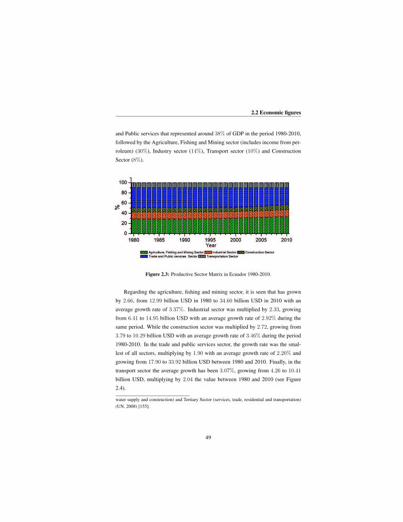
2.2 Economic figures
and Public services that represented around 38% of GDP in the period 1980-2010,
followed by the Agriculture, Fishing and Mining sector (includes income from pet-
roleum) (30%), Industry sector (14%), Transport sector (10%) and Construction
Sector (8%).
Figure 2.3: Productive Sector Matrix in Ecuador 1980-2010.
Regarding the agriculture, fishing and mining sector, it is seen that has grown
by 2.66, from 12.99 billion USD in 1980 to 34.60 billion USD in 2010 with an
average growth rate of 3.37%. Industrial sector was multiplied by 2.33, growing
from 6.41 to 14.95 billion USD with an average growth rate of 2.92% during the
same period. While the construction sector was multiplied by 2.72, growing from
3.79 to 10.29 billion USD with an average growth rate of 3.46% during the period
1980-2010. In the trade and public services sector, the growth rate was the smal-
lest of all sectors, multiplying by 1.90 with an average growth rate of 2.20% and
growing from 17.90 to 33.92 billion USD between 1980 and 2010. Finally, in the
transport sector the average growth has been 3.07%, growing from 4.26 to 10.41
billion USD, multiplying by 2.04 the value between 1980 and 2010 (see Figure
2.4).
water supply and construction) and Tertiary Sector (services, trade, residential and transportation)
(UN, 2008) [155].
49

2. ECUADOR IN FIGURES (1980-2010)
Figure 2.4: Top: Evolution of income by productive sector in Ecuador 1980-2010.
Bottom: Growth rate.
2.3 Energy figures
The analyzed historical data (1980-2010) indicates that Ecuador has become a net
exporter of energy but not self-sufficient. The structure of the processing plants, re-
fineries specifically, is inadequate in relation to the composition of the local market,
preventing meet energy needs. The request is subject to population growth, eco-
nomic development and technological advancement. Ecuador, like other countries
in the region, does not have complete information and data of its energy potential.
The country energy transition has followed, in general terms, the global trends.
The substitution of primary energy supply registered a loss of penetration of the
wood on fossil fuels and moderate growth of hydropower. The choice of oil as the
main source of energy supply makes the country very vulnerable energetically. The
relative abundance of this resource has reduced the prospects for increasing the use
of other technologies and diversification of the energy matrix. Despite the high
50
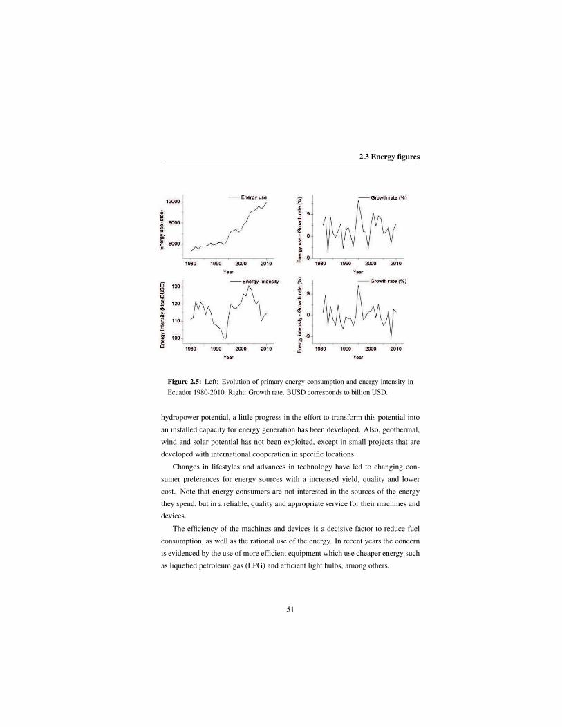
2.3 Energy figures
Figure 2.5: Left: Evolution of primary energy consumption and energy intensity in
Ecuador 1980-2010. Right: Growth rate. BUSD corresponds to billion USD.
hydropower potential, a little progress in the effort to transform this potential into
an installed capacity for energy generation has been developed. Also, geothermal,
wind and solar potential has not been exploited, except in small projects that are
developed with international cooperation in specific locations.
Changes in lifestyles and advances in technology have led to changing con-
sumer preferences for energy sources with a increased yield, quality and lower
cost. Note that energy consumers are not interested in the sources of the energy
they spend, but in a reliable, quality and appropriate service for their machines and
devices.
The efficiency of the machines and devices is a decisive factor to reduce fuel
consumption, as well as the rational use of the energy. In recent years the concern
is evidenced by the use of more efficient equipment which use cheaper energy such
as liquefied petroleum gas (LPG) and efficient light bulbs, among others.
51

2. ECUADOR IN FIGURES (1980-2010)
The consumption of primary energy by the country have increased by 2.37
between 1980 and 2010, going from 5032 to 11931 kt of oil equivalent (ktoe) (see
Figure 2.5). Global energy intensity has a fluctuating evolution and the average
value is 116 ktoe/BUSD in the period 1980-2010 (see Figure 2.5).
2.3.1 Energy matrix and energy intensity by sectors
Agriculture, fishing and mining sector uses mainly gasoline and diesel [154] and
historically is the least energy-intensive sector. It represents less than 5% within
the energy matrix by sector (see Figure 2.6), showed decreasing trend in the 1980s,
with a subsequent stabilization in the following years. The average growth rate is
1.14% but the historical data shows a decline in the use of energy going from 151
ktoe in 1980 to 123 ktoe in 2010 (see Figure 2.7). The energy intensity in the sector
is the lowest of all sectors, with a clear downward trend that leds its value from 11.6
to 3.57 ktoe/BUSD between 1980 and 2010 (see Figure 2.8).
In the industrial sector, energy consumption appears less concentrated (regard-
ing the source), due to the characteristics of each production process in various
industries. In the first decade of the 21st century, the use of fuel oil predominates
(35%), followed by the use of diesel oil (21%), cane products (20%) and finally
electricity (15%), while the wood lost penetration (Mosquera, 2008) [154]. Fossil
fuels and electricity are used to provide power to industrial cycles for generating
prime mover and heat. However, these activities have low productivity per unit of
energy, derived from the technologies used, which affects the competitiveness of
Ecuadorian products in the international market.
Energy consumption in the industrial sector accounts for about 21% of the en-
ergy matrix by sector (see Figure 2.6). The amount of energy used by the sector
increased from 856 to 2565 ktoe between 1980 and 2010 (see Figure 2.7). Energy
intensity of the sector indicates a fluctuating evolution around an upward trend
with a peak of 250 ktoe/BUSD in 2004 that was originated because the fuel mix
and the lower efficiency of the technologies used. Since 2005 the sector has shown
a shift in energy intensity, leading this intensity to a much lower value in 2010, 172
ktoe/BUSD (see Figure 2.8).
52
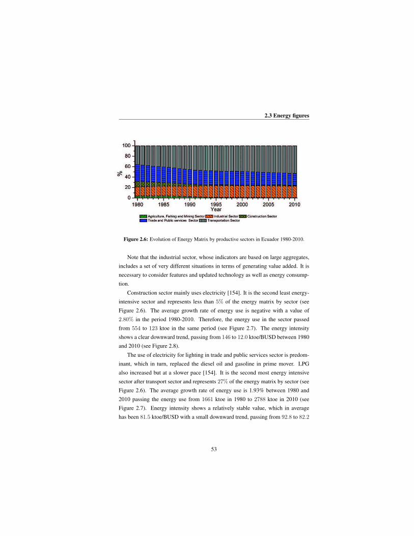
2.3 Energy figures
Figure 2.6: Evolution of Energy Matrix by productive sectors in Ecuador 1980-2010.
Note that the industrial sector, whose indicators are based on large aggregates,
includes a set of very different situations in terms of generating value added. It is
necessary to consider features and updated technology as well as energy consump-
tion.
Construction sector mainly uses electricity [154]. It is the second least energy-
intensive sector and represents less than 5% of the energy matrix by sector (see
Figure 2.6). The average growth rate of energy use is negative with a value of
2.80% in the period 1980-2010. Therefore, the energy use in the sector passed
from 554 to 123 ktoe in the same period (see Figure 2.7). The energy intensity
shows a clear downward trend, passing from 146 to 12.0 ktoe/BUSD between 1980
and 2010 (see Figure 2.8).
The use of electricity for lighting in trade and public services sector is predom-
inant, which in turn, replaced the diesel oil and gasoline in prime mover. LPG
also increased but at a slower pace [154]. It is the second most energy intensive
sector after transport sector and represents 27% of the energy matrix by sector (see
Figure 2.6). The average growth rate of energy use is 1.93% between 1980 and
2010 passing the energy use from 1661 ktoe in 1980 to 2788 ktoe in 2010 (see
Figure 2.7). Energy intensity shows a relatively stable value, which in average
has been 81.5 ktoe/BUSD with a small downward trend, passing from 92.8 to 82.2
53

2. ECUADOR IN FIGURES (1980-2010)
Figure 2.7: Top: Evolution of energy use by productive sectors in Ecuador 1980-2010.
Bottom: Growth rate.
ktoe/BUSD between 1980 and 2010 (see Figure 2.8).
The residential energy consumption that is included in this sector, shows a sig-
nificant drop in firewood consumption and an increase in penetration of the LPG
and electricity. LPG is dominant in houses for various uses such as water heating
and cooking, especially in isolated areas without electricity. The downward trend
in the average energy intensity of the residential sector is a reflection of a historical
process of improvement in household equipment that has allowed the replacement
of inefficient energy sources by others more efficient [154].
The transport is the most energy-intensive sector, accounting for nearly 50% of
the country’s energy use (see Figure 2.6). With a clear upward trend and it has in-
creased its consumption by 3.50 going from 1812 ktoe in 1980 to 6332 ktoe in 2010
(see Figure 2.7). It is also the largest consumer of liquid fuels. There is a significant
fall in the use of gasoline in favor of oil diesel, as a result of the increase use of
54

2.3 Energy figures
Figure 2.8: Top: Evolution of energy intensity by productive sectors in Ecuador 1980-
2010. Bottom: Growth rate.
internal combustion engines in freight transport (trucks) and passenger (buses) for
middle and long distance (Mosquera, 2008) [154]. The growth of the national fleet
has given increasing consumption of gasoline and diesel oil, helped by subsidized
prices of these fuels, which are still below the average values of the region. On the
other hand, it is observed that energy intensity fluctuates around 550 ktoe/BUSD,
with a slightly increasing trend and much higher levels than in the case of industry
(see Figure 2.8).
As mentioned above, this sector is the largest energy consumer in the country
(about 50% of energy consumption), but it represents only 10% in the generation
of income. Transport sector is intensive in the use of energy and shows signs of
inefficiency arising from inadequate modal distribution to meet the demand of pas-
sengers and freight transport.
55

2. ECUADOR IN FIGURES (1980-2010)
2.3.2 Energy matrix by sources
Figure 2.9: Evolution of Energy Matrix by energy source in Ecuador 1980-2010.
The energy matrix by sources is composed by the following primary energy
sources: i) Fossil fuel comprising coal, oil, petroleum, and natural gas products.
ii) Alternative and nuclear energy, refers to clean energy that is non-carbohydrate
energy and does not produce carbon dioxide when generated. It includes hydro-
power, geothermal, and solar power, among others. iii) Combustible renewables
and waste that comprise solid biomass, liquid biomass, biogas, industrial waste,
and municipal waste (WB, 2012) [146].
Following the trend of the region and most of the world, in Ecuador there is a
strong dependence on fossil fuels, which represents more than 80% of the energy
matrix in the period from 1980 to 2010 and has reached a peak of 88% in 2010 (see
Figure 2.9).
The use of alternative energy sources has had a very poor increase going from
1.22% to 7.06% (see Figure 2.9) in the national energy matrix between 1980 and
2010.
Furthermore, renewable and waste fuel have presented a considerable reduction
passing from 19.7% in 1980 to only 4.9% of the energy matrix in 2010 (see Figure
56
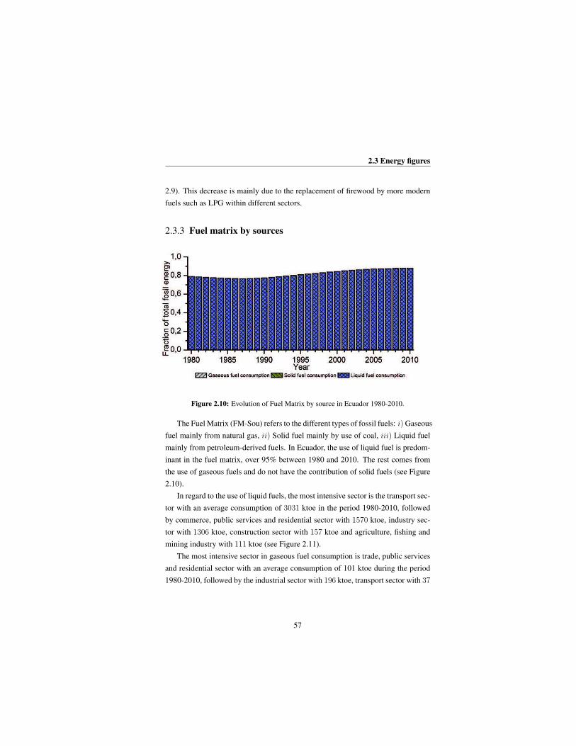
2.3 Energy figures
2.9). This decrease is mainly due to the replacement of firewood by more modern
fuels such as LPG within different sectors.
2.3.3 Fuel matrix by sources
Figure 2.10: Evolution of Fuel Matrix by source in Ecuador 1980-2010.
The Fuel Matrix (FM-Sou) refers to the different types of fossil fuels: i) Gaseous
fuel mainly from natural gas, ii) Solid fuel mainly by use of coal, iii) Liquid fuel
mainly from petroleum-derived fuels. In Ecuador, the use of liquid fuel is predom-
inant in the fuel matrix, over 95% between 1980 and 2010. The rest comes from
the use of gaseous fuels and do not have the contribution of solid fuels (see Figure
2.10).
In regard to the use of liquid fuels, the most intensive sector is the transport sec-
tor with an average consumption of 3031 ktoe in the period 1980-2010, followed
by commerce, public services and residential sector with 1570 ktoe, industry sec-
tor with 1306 ktoe, construction sector with 157 ktoe and agriculture, fishing and
mining industry with 111 ktoe (see Figure 2.11).
The most intensive sector in gaseous fuel consumption is trade, public services
and residential sector with an average consumption of 101 ktoe during the period
1980-2010, followed by the industrial sector with 196 ktoe, transport sector with 37
57

2. ECUADOR IN FIGURES (1980-2010)
ktoe, construction sector with 10 ktoe and agriculture, fishing and mining industry
with 7 ktoe (see Figure 2.11).
Figure 2.11: Evolution of Fuel consumption by productive sectors in Ecuador 1980-
2010. Top: Liquid fuel consumption. Down: Gaseous fuel consumption. Note that
there is not consumption of solid fuel in the country.
2.4 Emissions figures
Ecuador has had a modest but steady increase in CO2 emissions1, mainly due to the
increase of population and the growht of the economy, changing habits and more
frequent use of devices that require more energy in the different productive sectors
of the country. Emissions have increased by 2.37 between 1980 and 2010, passing
1CO2 represents 76.7% of the GHG emissions (approximately 56.6% is from fossil fuels,
17.3% from deforestation, and 2.8% from other sources) (IPCC, 2007) [156], in this dissertation all
CO2 data correspond to burning of fossil fuels
58
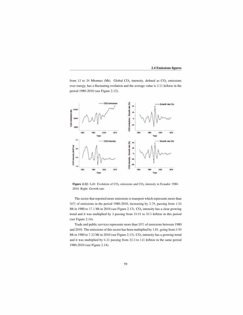
2.4 Emissions figures
from 12 to 28 Mtonnes (Mt). Global CO2 intensity, defined as CO2 emissions
over energy, has a fluctuating evolution and the average value is 2.51 kt/ktoe in the
period 1980-2010 (see Figure 2.12).
Figure 2.12: Left: Evolution of CO2 emissions and CO2 intensity in Ecuador 1980-
2010. Right: Growth rate.
The sector that reported more emissions is transport which represents more than
50% of emissions in the period 1980-2010, increasing by 3.79, passing from 4.50
Mt in 1980 to 17.1 Mt in 2010 (see Figure 2.13). CO2 intensity has a clear growing
trend and it was multiplied by 3 passing from 19.81 to 59.5 kt/ktoe in this period
(see Figure 2.14).
Trade and public services represents more than 20% of emissions between 1980
and 2010. The emissions of this sector has been multiplied by 1.81, going from 3.99
Mt in 1980 to 7.22 Mt in 2010 (see Figure 2.13). CO2 intensity has a growing trend
and it was multiplied by 6.31 passing from 22.3 to 141 kt/ktoe in the same period
1980-2010 (see Figure 2.14).
59

2. ECUADOR IN FIGURES (1980-2010)
Figure 2.13: Top: Evolution of CO2 emissions by productive sectors in Ecuador 1980-
2010. Bottom: Growth rate.
Industry sector represents accounts for about 20% of emissions between 1980
and 2020. This sector has increased by 3.20, going from 2.19 Mt in 1980 to 6.99 Mt
in 2010 (see Figure 2.13). This sector has the second largest growth after transport-
ation. CO2 intensity also has a growing trend and was multiplied by 5.32 passing
from 10.8 to 57.6 kt/ktoe between 1980 and 2010 ( see Figure 2.14).
The aggregation of agriculture, fishing and mining sector and construction sec-
tor both represents less 10% of emissions between 1980 and 2020. In addition,
both sectors have decreased their emissions. Agriculture, fishing and mining sector
emissions were multiplied by 0.67 and construction sector by 0.26, going from 0.49
to 0.32 Mt and from 1.32 to 0.34 Mt respectively in the same period (see Figure
2.13). In CO2 intensity, there is a significant difference between both sectors, while
the agriculture, fishing and mining sector has keep an almost constant intensity of
2.48 kt/ktoe for the period 1980-2010, the construction sector has shown a clear
60

2.4 Emissions figures
downward trend, from 6.53 to 2.78 in the same period. (see Figure 2.14).
Figure 2.14: Top: Evolution of CO2 intensity in Ecuador 1980-2010. Bottom: Growth
rate.
Now we disaggregated emissions by type of fossil fuel and by sector. Regarding
emissions from gaseous fuel, the most intensive sector is trade, public services
and residential sector with an average emission of 237 kt during the period 1980-
2010, followed by the industrial sector with 196 kt, transport sector with 87.1 kt,
construction sector with 20.2 kt and agriculture, fishing and mining industry with
15.5 kt (see Figure 2.15).
In regard to emissions by liquid fuels, the most intensive sector is the transport
sector with an average emission of 5306 kt in the period 1980-2010, followed by
trade, public services and residential sector with 4819 kt, industry sector with 4009
kt, construction sector with 483 kt and agriculture, fishing and mining industry with
17.1 kt (see Figure 2.15).
61

2. ECUADOR IN FIGURES (1980-2010)
Figure 2.15: Top: Evolution of CO2 emissions by fuel in Ecuador 1980-2010. Bot-
tom: Growth rate. Note that there is not consumption of solid fuel in the country.
2.5 Renewable energy figures
The Ecuadorian government has, among its goals, the development of strategies
to guarantee the energy supply, increase energy cost efficiency, and last, but not
least, to minimize the negative impact of economic development on the environ-
ment (Mosquera, 2008) [154].
Renewable energy sources could play an important role in the diversification
of the energy matrix in Ecuador. In particular, CONELEC-004 /11 regulation
(Conelec, 2011) [157] establishes the conditions for selling electricity from renew-
able sources to the national grid, which is encouraging new projects. Below we
summarize projects and potential sources that could increase the use of renewable
energy in Ecuador in the upcoming years.
62
2.5 Renewable energy figures
2.5.1 Bioenergy
Ecuador has a good potential to use modern, clean and efficient bioenergy techno-
logies using diverse crop and livestock production to generate waste energy. The
type of animal waste can be harnessed through anaerobic digestion to produce bio-
gas (methane) (Conelec, 2009) [3].
The country has about 71 thousand ha (2009) of sugarcane mostly concentrated
in the cost region, near Guayaquil (MAG, 2011) [158]. A fuel ethanol pilot program
has been planned in Guayaquil and Quito, initially consisting of 5% ethanol blend
with gasoline [159]. If it is successful, this could set the ground for a nation-wide
ethanol fuel program. The use of this kind of fuel will generate savings of about
32 million USD a year, as the country would stop importing about 320 thousand of
barrels of high octane naphtha1 (15%) (MEER, 2011) [159].
On the other hand, the total area planted with African palm in Ecuador is
240 thousand ha, with about 200 thousand ha currently being harvested [158].
Ecuador could potentially plant up to 760 thousand ha of African palm according
to Ecuador’s Association of African Palm Growers (ANCUPA, 2013) [160]. Based
on projections from the sector in terms of production, domestic consumption and
export surplus of red oil, the surplus could grow significantly and reach more than
850 kt of red oil in 2025 (USDA, 2011) [161].
In Ecuador, more than 300 thousand tonnes of husk is produced annually. A
tonne of this residue has the ability to displace the consumption of 90 gallons of
diesel used in steam generation for both processing and food production. So the
300 thousand tonnes would reduce the use of about 27 million gallons of diesel a
year, besides avoiding the emission of CO2 and other primary pollutants (Neira et
al., 2006) [162].
Note that, according to the cycle of sugar cane harvest, these plants operate with
variability in their production. The annual average load factor in 2010 was 29%.
During the months of August to November has come to be greater than 60% while
between January and April has not been operated for lack of waste (Conelec, 2011)
[157]. The implementation of these initiatives require institutional efforts and that
1Naphtha is used primarily as feedstock for producing high octane gasoline.
63
2. ECUADOR IN FIGURES (1980-2010)
the market offers the conditions for collection and storage of husk, combined with
incentives to the diffusion of technology in rural areas.
2.5.2 Geothermal energy
Ecuador is a country with active volcanism that is part of the Pacific Ring of Fire
and has a great geothermal potential. This is illustrated by the presence of around
180 hot springs in the country and a geothermal potential of 534 MW (CEPAL,
2010) [163]. Studies have identified 17 potential geothermal exploitation for pro-
duction of electrical, industrial and agricultural energy (Conelec, 2009) [3].
Three sites, Tufino-Chiles (139 MW), Chachimbiro (113 MW) and Barges (282
MW) in which has been quantified an installable power of 534 MW. The Chalupas
geothermal project has been determined like priority. This project is in the feasib-
ility stage (2011) and it requires further geophysical exploratory work to bring it to
the next stage. The cost of exploration and feasibility stage represents 10% of the
total budget. When this feasibility is confirmed, additional drilling are required.
Then, stages of design, construction and installation should continue. These stages
would be the most expensive, arround 90% of the budget (Conelec, 2009) [3].
The loading factors at the global level are between 60% and 90%; which are
considered efficient levels of use of the resource (levels of basic energy source).
Geothermal has an advantage over other renewable: short term variable techno-
logies (solar, wind, wave and tidal), and hydroelectricity where load factors are
between 40% and 80% (Bruckner et al., 2011) [4].
2.5.3 Hydropower
As was mentioned above, Ecuador has a huge hydroelectric potential unexploited,
despite that hydropower is the renewable resource more exploited in the country. In
2011 Ecuador had 2, 215 MW of installed hydropower capacity and another 2, 756
MW under construction (Conelec, 2013) [164]. The biggest hydroelectric project
is called Coca Codo Sinclair and has a capacity of 1500 MW and an estimated cost
of 2.25 billion USD (the overall project progress is 27.4% up to November 2012).
Other hydroelectric projects are: Deisitanisagua with 115 MW, Maduriacu with 60
64
2.5 Renewable energy figures
MW, Mazar Dudas with 21 MW, Minas de San Francisco with 270 MW, Quijos
with 50 MW, Sopladora with 487 MW, and Toachi Pilaton with 253 MW [159].
2.5.4 Solar energy
The potential of this energy in Ecuador is not among the highest in the world,
compared to countries with high desert irradiations (e.g. North Africa), however,
it is at an appropriate level to become a significant source of national power. Note
that solar radiation is uniform throughout the year in Ecuador, which reduces the
problem of variations, and makes the use of technology more reliable (Conelec,
2009) [3].
Most of the Ecuadorian territory has an average annual potential of 4.4 to 4.7
kWh/m2/day solar radiation. Among the places with the most potential are Quito
(5.1 kWh/m2/day), Sigchos and Pedernales (5.25 kWh/m2/day), southern (5.25
kWh/m2/day) and west (5.4 kWh/m2/day) of Zapotillo and Macara (5.5 kWh/m2/day)
(CIE, 2008) [165]. Considering that it requires direct radiation of at least 5 kWh/m2/day
in order to be able to generate electricity from concentrated solar power (CSP)
(WB, 2010a), there are few places in the country to exploit this technology as is the
case of Macara in the south of Loja (5.1 kWh/m2/day direct sunlight) (CIE, 2008)
[165].
In addition, through Rural Electrification and Urban Marginal Funds (Fondos
de Electrificacion Rural y Urbano Marginal-FERUM), Ecuador initiated in 2004
a program of electrification in the countryside using PV generation units. This
program started in zones near the border with Peru and in the Amazonian region.
Another program using PV (Photovoltaic) panels is executed in the Galapagos Is-
lands to generate a power of 2.1 MW (MEER, 2011) [159].
2.5.5 Wave and tidal energy
There are no reviews or studies in Ecuador about the potential of this energy. The
Expansion Master Plan 2009-2020 states that a wave and tidal potential in the coun-
try could be and it can be used as an energy option in places close to the coast.
Global information estimated a moderate potential of this type of energy for the
65

2. ECUADOR IN FIGURES (1980-2010)
Ecuadorian coast (between 15 and 16 kW per meter of wave), which is low com-
pared to sites with high potential as southern Chile with 74 kW/m.
Load factors of this energy are between 22.5% and 28.5%, which shows its
variable nature. Note that, the useful life of tide dams is about 40 years. In order
to integrate these energies to the system, it is required to expand the transmission
infrastructure near the coast, or even a few kilometers off to the coast if the gen-
erators are located offshore. The electrical characteristics of the power plants of
both waves and tides is similar to those of wind energy technologies, therefore, the
technical connection requirements are often similar (Sims et al., 2011) [24].
2.5.6 Wind energy
A challenge for the integration of wind energy to electrical systems is their inter-
mittent nature for the energy generation (Arent, 2011) [2]. That is, the wind is
a variable resource so that the generation fluctuates according to weather condi-
tions and wind in a given plant or wind turbine. When wind electricity generation
represents more than 20% of country’s electricity matrix, it requires technical and
institutional adjustments by the authority (Wiser et al, 2011 [14]; Taylor, 2004
[166]).
Although latitudes located on the equator are not rich in winds, the presence of
the Andes Mountains and the Pacific Ocean provide thermal gradients that allow
the existence of areas of high wind interest in Ecuador. To determine the potential
of wind generation site, it is required to evaluate different parameters such as wind
speed, daily, monthly and seasonal variations. Wind energy is one of the most
variable renewable sources in the short term (Sims et al., 2011) [24], and even
more than solar, because the wind varies dramatic and randomly.
The areas with the highest wind potential in Ecuador are at the tops of the moun-
tains and coastal sites. Among these sites Villonaco hill located in the province of
Loja in the south of the country is recognized, with a cost of 41.8 million USD, a
power capacity of 16.5 MW and considered in the Plan of Expansion of Generation
2009-2020 of Ecuador. There are some other identified sites with wind generation
potential, such as The Angel in Carchi, Salinas in Imbabura, Tixan in Chimborazo
66

2.6 Cost of the adoption of renewable energy
and Huascachaca in Azuay. A specific technical evaluation, both national and local
levels to get a full wind atlas of the country is still required (Conelec, 2009) [3].
Programs for using wind energy started in 2004. Other important program,
promoted by the Ministry of Electricity and Renewable Energy (MEER), aim at re-
placing the existing thermal generation plant by wind and PV plants in the Galapa-
gos Islands. With the new facilities, 5.7 MW of wind power (plus 2.1 MW of
PV power) will substitute most of the 8.8 MW of the thermal generation installed
(MEER, 2011 [159]; Conelec, 2013 [164]).
2.6 Cost of the adoption of renewable energy
The cost of renewable energy is an important factor in determining the competit-
iveness of a given technology in the energy sector. Thus, if a technology generates
electricity at below market price, estimated for the long term, this technology would
be selected by investors for future expansion (Caspary, 2009) [167]. Costs are still
a critical factor, then, it is most feasible and likely to adopt technologies that have
competitive costs compared to the traditional electricity sector.
This section compares overall average technology costs ranges of renewable en-
ergy with the costs paid to electricity generators in Ecuador. The average costs of
renewable energy generation technologies are taken from IPCC1. The data corres-
pond to the global aggregate costs of renewable energy technologies commercially
available.
Further, costs are not the only factor used but also the commercial availability of
technologies. These cost ranges are constructed based on information from coun-
tries where there are projects, studies and information on these technologies. Also,
are listed the natural and technological factors affecting the feasibility of using each
type of renewable source such as load factor (which expresses the variability and
natural availability of a source), life-cycle and size of the plant, and costs incurred
in investment, operation, maintenance and fuel (for bioenergy).
1The average costs of technologies for renewable energy sources given by the IPCC are cal-
culated for the life-cycle of each of the technologies and are calculated at present value with a
discount rate of 7%. None of these average costs include effects of energy subsidies granted in
different countries (Bruckner et al 2011) [4].
67

2. ECUADOR IN FIGURES (1980-2010)
Figure 2.16: International average cost range versus preference prices for renewable
energy in Ecuador based on (Conelec 2009) [3] and (Bruckner et al 2011) [4].
The comparison of cost is a first step in the analysis of the feasibility of incor-
porating renewable technologies in the energy matrix of the country. Moreover,
the comparative cost used is the generation of electricity in Ecuador determined by
Conelec1 (Conelec, 2009)[3].
Figure 2.16 shows that four technologies of renewable energy would have in-
centives to be adopted without the support of preferential prices2. These technolo-
gies show a global average cost range lower than the recognized power generation
1 In 2011 a new regulation of Conelec (Regulation No. CONELEC-004/11) was approved for
the treatment of the price of energy produced from non-conventional renewable energy resources,
which seeks to encourage the spread of these technologies in Ecuador through the payment of
preferential prices to allow greater competitiveness thereof. The costs of electricity generation of
Conelec are average values of domestic industries (Conelec 2009) [3]2 The Conelec’s regulation (feed in tariff) contributes to the adoption of technologies of re-
newable energy in Ecuador’s electricity market. These regulations provide for different preferential
prices for different technologies (see the different lines in Figure 2.16). Technologies that have their
range of prices below these ceilings become economically viable energy in Ecuador.
68
2.6 Cost of the adoption of renewable energy
in Ecuador (range of cost below the red line in the graph) cost. These technolo-
gies are: bioenergy for electricity generation by combined combustion (co- firing),
gasification of biomass for heat and power generation (combined heat and power,
CHP); geothermal flash steam technologies (flash condensing plants) and binary
cycle plants.
The regulation of preferential prices govern the payment of costs for a period
of 15 years, after which the authority will conduct a review. With this time horizon
and with the downward trend in the cost of renewable technologies is likely that
more options will become financially viable in the medium and long term.
The energy generation based on fossil fuels produces global effects such as
GHG and local effects such as the emission of primary pollutants (eg SOx, NOx,
etc.). If these effects are incorporated, the real cost of power generation from these
sources will be higher. Then, renewable technologies produces least amount and
less intense effects, especially in GHG. This option would become more competit-
ive in front of polluter energy generation.
Since the incorporation of these effects are not included in the price of energy
generation in Ecuador, we can only refer to the financial costs. Note that this fin-
ancial cost of energy generation is not the actual cost, because the energy sector
(especially the thermoelectric generation) use subsidized fuel. These factors, sub-
sidies for fossil fuels and non-inclusion of external environmental costs make the
price of conventional energy generation technologies in Ecuador cheaper than re-
newable energy sources. However, the low price is not based on real and sustainable
benefits in the long term.
Regarding energy costs for transportation, there is a global downward trend
in the prices of first generation biofuels (see Figure 2.16). Particularly in Latin
America, Brazil is the leader in biofuels production, and is achieving lower cost
and not requiring subsidies to be competitive (Chum et al., 2011) [18]. But in
Ecuador, gasoline and diesel have costs below the world average price and even
below that of its Andean neighbors, Peru and Colombia, because of subsidies.
69


Education is the most powerful
weapon which you can use to
change the world.
Nelson Mandela
CHAPTER
3System dynamics modelling
for renewable energy and
CO2 emissions in Ecuador
(1980-2025)
3.1 Overview
It is a very complicated task to predict how much the economy will grow in the
near future. This growth will strongly modulate CO2 emissions of any coun-
try and therefore it will be crucial to make a realistic estimate of this emissions.
On the other hand, the different feedback-mechanisms, both in the climatic and in
the economic system make any prediction highly questionable beyond 5-10 years
(Fiddman, 2002) [82]. However, it is critical to provide accurate information to
policymakers in order to design appropriate energy policies for the near future
(Bahrman, 2007) [168].
This Chapter explores the relationship between economic growth, productive
sectors, energy consumption, changes in the use of renewable energy, improve-
ments in the efficiency of fossil energy, and CO2 emissions of Ecuador. To estimate
71
3. SYSTEM DYNAMICS MODELLING FOR RENEWABLE ENERGY
AND CO2 EMISSIONS IN ECUADOR (1980-2025)
CO2 emissions in the near future we will define different scenarios in both income
and energy use.
The model is based on a variation of the Kaya identity (Kaya, 1993) [169]
and on an approach of formation of GDP which includes a contribution from re-
newable energy (Chien and Hu) [5]. The model has been implemented using a
SD technique (Forrester, 1961) [170] on a Vensim platform (Vensim, 2011) [171].
The considered data corresponds to the period 1980-2010 and it has been extrac-
ted from the official data sources such as: Ecuadorian Institute of Statistics and
Census (INEC, 2012) [172], Central Bank of Ecuador (BCE) [152], World Bank1
(WB) [146], and International Energy Agency (IEA) [153]. The raw data has been
processed using a Hodrick-Prescott filter (HP) (Hodrick and Prescott, 1997) [173]
which allows to generate a smooth representation of a time series.
The Kaya identity is commonly used as an analytical tool to explore the main
driving forces that control the amount of carbon dioxide emissions (Alcantara, 2005
[174]; Mena, 2009 [175]). According to this identity, CO2 emissions of a given
country could be broken down into the product of four factors: carbon intensity
(defined as the CO2 emitted per unit of energy consumed), energy intensity (defined
as the consumed energy per unit of GDP), economic rent (defined as GDP per
capita), and population.
The technique was originally proposed by J. Forrester to understand how sys-
tems change as a function of time (Begueri, 2001) [176]. SD is a method for
modeling, simulating and analyzing complex systems. A system is defined as a
collection of elements in which interactions are modeled as flows between reser-
voirs in time steps, and in which the rate of change depends on the value of the
variables that define the system (feedback mechanisms). Therefore, the main goal
of SD is to understand how a given system evolves, and even more importantly, to
understand the causes that govern its evolution (Garcia, 2011) [86]. The basis of
SD has been analyzed in detail in Radzicki (2009) [177] and Tan (2010) [178], in
addition a brief review is in Section 1.9 of Chapter 1.
1Economic official data set used is given in constant 2005 PPP international dollars.
72

3.2 Formulation of model
3.2 Formulation of model
The model uses a variation of the Kaya identity, where the amount of CO2 emis-
sions from industry and from other energy uses may be studied quantifying the con-
tributions of five different factors: i) global industrial activity, ii) industry activity
mix, iii) sectoral energy intensity, iv) sectoral energy mix and v) CO2 emission
factors. Moreover, we consider different sub-categories concerning the industrial
sectors and the fuel type. The CO2 emissions can be written as,
C =∑
ij
Cij =∑
ij
QQi
Q
Ei
Qi
Eij
Ei
Cij
Eij
=∑
ij
Q · Si · EIi ·Mij · Uij, (3.1)
where C is the total CO2 emissions (in a given year); Cij is the CO2 emission
arising from fuel type j in the productive sector i (note that the index i runs over
five productive sectors and the index j over five type of energy sources); Q is the
total GDP of the country; Qi is the GDP generated by the productive sector i; Ei is
the energy consumption in the productive sector i; Eij is the consumption of fuel j
in the productive sector i, verifying that the total consumed energy, E =∑
ij Eij;
Si
(
Qi
Q
)
is the share of sector i in the total GDP; the energy intensity of sector i is
given by EIi
(
Ei
Qi
)
; the energy matrix is given by Mij
(
Eij
Ei
)
and the CO2 emission
factor by Uij
(
Cij
Eij
)
. Throughout this work, as a convention, we will always refer
to the productive sector with the i index and to the type of energy source with the j
index.
This equation is an extension of the Kaya identity because we disaggregate in
type of productive sector and kind of fuel used, while in the original formulation
only aggregated terms are considered: C, Q, and E.
The raw data to perform the model correspond to the official available data on
Ecuador, provided by the INEC1, the BCE2, the WB3, and the International Energy
Agency4. The subsequent data analysis and the preprocessing of the time series
was performed using the Hodrick-Prescott (HP) filter [173], which allows isolation
1http:// www.inec.gob.ec/estadisticas/, http://www.ecuadorencifras.com/2http://www.bce.fin.ec/indicador.php3http://data.worldbank.org/country/ecuador4http://www.iea.org/ countries/non-membercountries/ecuador/
73
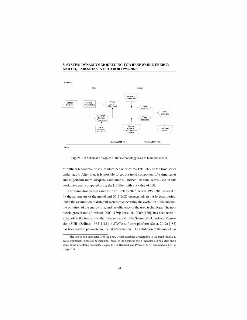
3. SYSTEM DYNAMICS MODELLING FOR RENEWABLE ENERGY
AND CO2 EMISSIONS IN ECUADOR (1980-2025)
Figure 3.1: Schematic diagram of the methodology used to build the model.
of outliers (economic crises, random behavior of markets, etc) of the time series
under study. After that, it is possible to get the trend component of a time series
and to perform more adequate estimations1. Indeed, all time series used in this
work have been computed using the HP filter with a λ value of 100.
The simulation period extends from 1980 to 2025, where 1980-2010 is used to
fix the parameters of the model and 2011-2025 corresponds to the forecast period,
under the assumption of different scenarios concerning the evolution of the income,
the evolution of the energy mix, and the efficiency of the used technology. The geo-
metric growth rate (Rowland, 2003 [179]; Jin et al., 2009 [180]) has been used to
extrapolate the trends into the forecast period. The Seemingly Unrelated Regres-
sion (SUR) (Zellner, 1962) [181] in STATA software platform (Stata, 2012) [182]
has been used to parameterize the GDP formation. The validation of the model has
1 The smoothing parameter λ of the filter, which penalizes acceleration in the trend relative to
cycle component, needs to be specified. Most of the business cycle literature use past data and a
value of the smoothing parameter λ equal to 100 (Hodrick and Prescott) [173] (see Section 1.5.3 in
Chapter 1).
74

3.3 Economic model approach
been done with the mean absolute percentage error (MAPE).
Figure 3.1 shows in a schematic way how the calculations have been performed
using the different techniques described in previous paragraphs.
3.3 Economic model approach
3.3.1 Introduction of economic appoach
The promotion of renewable energy is a well accepted solution to the mitigation of
CO2 emission. Furthermore, Chien and Hu (2007) [183] show that increasing the
use of renewable energy improves the macroeconomic efficiency of economies.
Energy, labor, and capital stock are key inputs to produce the economic output-
GDP (Hu and Kao, 2007 [184]; Hu and Wang, 2006 [185]). It is desirable for an
economy to increase its income and to decrease its inputs in order to maximize
production efficiency.
It is worth noting that increasing the input of traditional energy decreases tech-
nical efficiency. To improve the technical efficiency of an economy, it is important
not to increase the total input of energy. By substituting traditional energy with
renewable energy, technical efficiency can be improved (Hu and Kao, 2007) [183].
Renewable energy systems are considered to be environmentally superior to tra-
ditional technologies from the viewpoint of CO2 mitigation and the effective util-
ization of resources. Several studies show that substitution of conventional fossil
fuels by biomass, for energy production results, in both a net reduction of GHG
and in the replacement of non-renewable energy sources (Schneider and McCarl,
2003 [186]; Dowaki and Mori, 2005 [187]; Caputo et al., 2005[188]).
Abulfotuh (2007) [189] suggests that one possible solution to the environmental
risks brought by the escalating demand for energy is to consider immediate change
in the composition of the energy resource portfolio. It is expected that renewables
have great potential to solve a major part of global energy sustainability. Increasing
the use of renewables in power industries has already been seriously reviewed in
some countries.
Various new policies to achieve the national goals of a renewables ratio in the
energy portfolio are adopted in different economies. Lund (2007) [190] groups
75
3. SYSTEM DYNAMICS MODELLING FOR RENEWABLE ENERGY
AND CO2 EMISSIONS IN ECUADOR (1980-2025)
policies on renewable energy and efficient energy use into subsidy type and cata-
lyzes measures based on the use the public financial resources according to REN21
(Renewable Energy Policy for the 21st Century, 2012) [191] in Renewables Global
Status Report (RGSR, 2012) [191] at least 118 countries, more than half of which
are developing countries, had renewable energy targets in place, and 109 countries
have policies to support renewables in the power sector by early 2012. Renewable
energy targets and support policies continued to be a driving force behind increas-
ing markets for renewable energy, despite some setbacks resulting from a lack of
long-term policy certainty and stability in many countries.
Feed-in-tariffs (FITs) and renewable portfolio standards1 (RPS) are the most
commonly used policies in this sector. FIT policies were in place in at least 65
countries by early 2012 (REN, 2012) [191].
Renewables are currently accepted as one of the key solutions to climate change
and escalating energy demand. Many economies have adopting policies to promote
the use of renewables. However, the mechanism of how renewables improve GDP
is still unknown (Chien and Hu, 2008) [183].
3.3.2 Theory of the impact of renewables on GDP
In this section, we will review the work of Chien and Hu (2008) [5] that broadens
the perspective of environmental economics to include an analysis of renewable
usage directly contributing to the important elements of economies or regional de-
velopment. Domac et al. (2005) [192] suggest that renewable energy increases
the macroeconomic efficiency by the following process: i) The business expansion
and new employment brought by renewable energy industries result in economic
growth. ii) The import substitution of energy has direct and indirect effects in
increasing income of the economy and trade balance.
Measured by expenditures, GDP is the sum of goods and services produced dur-
ing a giving period. Total output comprises four groups’ purchases of final goods
1RPS is a regulation that requires the increased production of energy from renewable energy
sources, such as wind, solar, biomass, and geothermal. The RPS mechanism generally places an
obligation on electricity supply companies to produce a specified fraction of their electricity from
renewable energy sources. Certified renewable energy generators earn certificates for every unit of
electricity they produce and can sell these along with their electricity to supply companies.
76
3.3 Economic model approach
and services: i) households purchase consumption goods; ii) businesses purchase
investment goods (and retain unsold production as inventory increases); iii) gov-
ernments purchase goods and services used in public administration and iv) welfare
transfers; and foreigners purchase (net) exports. There is substantial uniformity in
the shares of consumption and investment (the sum of capital expenditures and in-
ventories) across nations with quite disparate income levels (Mack, 2008) [193]1. It is important to note that if one counts some major activities such as child-
rearing (generally unpaid) as production, GDP ceases to be an accurate indicator
of production. Similarly, if there is a long term shift from non-market provision
of services (for example cooking, cleaning, child rearing, do-it yourself repairs)
to market provision of services, then this trend toward increased market provision
of services may mask a dramatic decrease in actual domestic production, resulting
in overly optimistic and inflated reported GDP. This is particularly a problem for
economies which have shifted from production economies to service economies.
The expenditure approach estimates GDP by the following equation:
GDP = C + I +G+X −M, (3.2)
where:
• C (consumption) is normally the largest GDP component in the economy,
consisting of private (household final consumption expenditure) in the eco-
nomy. These personal expenditures fall under one of the following categor-
ies: durable goods, non-durable goods, and services. Examples include food,
rent, jewelry, gasoline, and medical expenses but does not include the pur-
chase of new housing.
• I (investment) includes, for instance, business investment in equipment, but
does not include exchanges of existing assets. Examples include construc-
tion of a new mine, purchase of software, or purchase of machinery and
equipment for a factory. Spending by households (not government) on new
houses is also included in investment. In contrast to its colloquial meaning,
investment in GDP does not mean purchases of financial products.
1Note that, if you knit yourself a socks, it is production but does not get counted as GDP because
it is never sold.
77

3. SYSTEM DYNAMICS MODELLING FOR RENEWABLE ENERGY
AND CO2 EMISSIONS IN ECUADOR (1980-2025)
• G (government spending) is the sum of government expenditures on final
goods and services. It includes salaries of public servants, purchases of
weapons for the military and any investment expenditure by a government.
It does not include any transfer payments, such as social security or unem-
ployment benefits.
• X (exports) represents gross exports. GDP captures the amount a country
produces, including goods and services produced for other nations’ con-
sumption, therefore exports are added.
• M (imports) represents gross imports. Imports are subtracted since imported
goods will be included in the terms G, I, or C, and must be deducted to avoid
counting foreign supply as domestic.
The deduction of imports from exports (X–M ) is the trade balance (TB).
Another way of measuring GDP is to measure total income (Income approach).
This way of counting is sometimes called gross domestic income (GDI1) and should
provide the same amount as the expenditure method described previously2
Following to Chien and Hu (2008) [5] the impact of renewables on GDP has
evaluated by the expenditure approach, because the import substitution effect of
renewables seems to have a direct impact on trade balance.
3.3.3 Path analysis of the impacts of renewables on GDP
The influences of renewables on GDP are illustrated by Figure 3.2. This represents
the original constitution of GDP by household consumption, government consump-
tion, capital formation, and trade balance.
Closely following Chien and Hu (2008) [5], in Figure 3.3, the diagram shows
that the use of renewables influences GDP through two paths: i) the emergence of
renewable energy industries brings business expansion, which results in increased
capital formation and ii) the import substitution of traditional energy by locally
1This method measures GDP by adding incomes of salaries for labour, interest for capital, rent
for land and profits for entrepreneurship.2By definition, GDI = GDP. In practice, however, measurement errors will make the two figures
slightly off when reported by national statistical agencies.
78

3.3 Economic model approach
Figure 3.2: Conceptual framework of GDP constitution in Chien and Hu (2008) [5]
produced renewables has direct and indirect effects on increasing trade balance in
an economy. The increases of capital formation and trade balance would lead to
the increase of the GDP.
Policy makers have to choose from different policy instruments to identify the
most effective instrument. This became very important issue and therefore the
mechanism for renewables to create economic impacts should be first identified.
Chien and Hu (2008) [5] use the path analysis of Structural Equation Model-
ing (SEM) to test the conceptual model, specifying causal relationships between
renewables and the other relevant variables 1. The output of path analysis in Chien
and Hu (2008) [5] work provides significance tests for specific causal paths. The
1Path analysis can be used to determine whether the theoretical model accounts for the actual
relationships in the observed data.
79
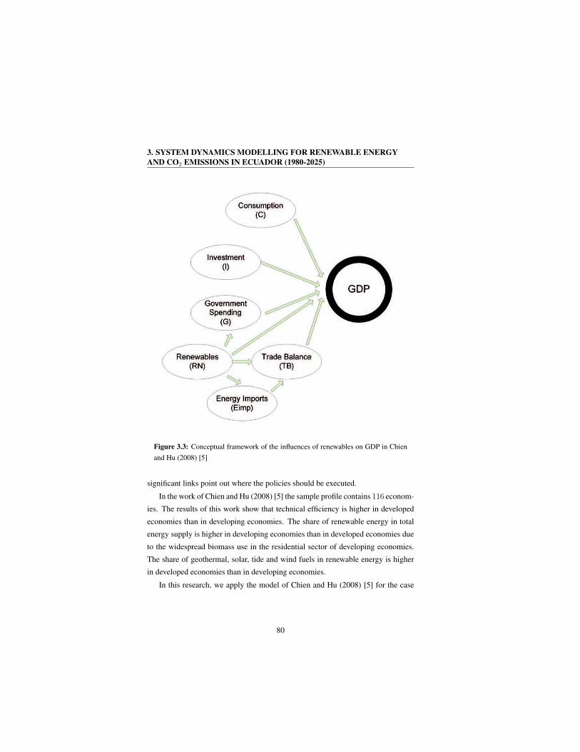
3. SYSTEM DYNAMICS MODELLING FOR RENEWABLE ENERGY
AND CO2 EMISSIONS IN ECUADOR (1980-2025)
Figure 3.3: Conceptual framework of the influences of renewables on GDP in Chien
and Hu (2008) [5]
significant links point out where the policies should be executed.
In the work of Chien and Hu (2008) [5] the sample profile contains 116 econom-
ies. The results of this work show that technical efficiency is higher in developed
economies than in developing economies. The share of renewable energy in total
energy supply is higher in developing economies than in developed economies due
to the widespread biomass use in the residential sector of developing economies.
The share of geothermal, solar, tide and wind fuels in renewable energy is higher
in developed economies than in developing economies.
In this research, we apply the model of Chien and Hu (2008) [5] for the case
80

3.3 Economic model approach
of Ecuador. We also conduct an analysis performed using the correlation matrix
(Table 3.1).
Table 3.1: Summary of descriptive statistics for the economic model.
Measure Means Stan.Dev GDP I TB C Eimp RN
GDPa 7.54 1.97 1.00 0.93 -0.12 0.97 -0.86 -0.86
Ib 1.71 0.54 0.93 1.00 -0.24 0.85 -0.67 -0.70
TBc -0.10 0.24 -0.12 -0.24 1.00 0.22 -0-05 0.02
Cd 5.00 1.37 0.97 0.85 -0.22 1.00 -0.89 0.87
Eimpe -12.72 3.81 -0.86 -0.67 -0.05 -0.89 1.00 0.87
RNf 3.81 0.18 -0.86 -0.70 0.02 -0.90 0.87 1.00
a GDP in 1010 USD.
b I in 1010 USD.
c TB in 1010 USD.
d C in 1010 USD.
e Eimp in 106 toe.
f RN in 106 toe.
On the other hand, according to these authors the government spending G (G =
GDP − C − I − (X − M)) is eliminated from the model estimation to avoid
multicollinearity. To avoid the problems of inputting raw data, a rescaling of the
smoothed time series has been used so that they are all on approximately the same
scale. The system of theoretical GDP formation model is made up by the following
equations:
Q = a1 · I + a2 · TB + a3 · C + a4 · Eimp+ a5 ·RN + ǫ1, (3.3)
I = b1 ·RN + b2 · C + ǫ2, (3.4)
TB = c1 · Eimp+ c2 ·RN + ǫ3, (3.5)
Eimp = d1 ·RN + ǫ4, (3.6)
C = f1 · Eimp+ f2 · TB + ǫ5, (3.7)
81
3. SYSTEM DYNAMICS MODELLING FOR RENEWABLE ENERGY
AND CO2 EMISSIONS IN ECUADOR (1980-2025)
where Q refers to GDP of the country, Eimp is the energy import, RN is the re-
newable energy and ǫ1... ǫ5 are residuals. Note that Equations 3.3-3.7 form the
model for the formation of GDP. Coefficients appearing in these equations are de-
termined using SUR technique1 in the datasets of 1980-2010 period and therefore
their values are a consequence of the data. The SEM model is present in Figure
3.4.
In Equation 3.3, income (Q) is influenced by invest (I), trade balance (TB),
and consumption (C). Chien and Hu (2007) [183] suggested that energy inputs
may affect income, therefore, energy imports (Eimp) and renewable energy (RN )
are included as well Equation (3.3). Note the negative value of coefficient a5 in
Table 3.2.
In Equation 3.4 investment is influenced by renewable energy, since theory pre-
dicts that increasing the use of renewable energy will result in business expansion
and thus capital could be accumulated in long term, but its implementation (infra-
structure and incentives in early stages, see Section 2.6 in Chapter 2) is expected
to have a negative short term effect over income (this is confirmed with a negative
value of b1 in Table 3.2).
In Equation 3.5 energy imports and renewable energy influence trade balance
(both coefficients, c1 and c2, have positive values in Table 3.2). The theory pro-
posed by Domac et al. (2005) [192] suggests that the use of renewable energy
results in import substitution by domestic-produced renewable energy, and thus
trade balance will increase by the use of renewable energy. Furthermore, if renew-
able energy could cause import substitution, then the imports of energy should be
1 A single model may contain a number of linear equations. In such a model it is often un-
realistic to expect that the equation errors would be uncorrelated. A set of equations that has con-
temporaneous cross-equation error correlation (i.e. the error terms in the regression equations are
correlated) is called a seemingly unrelated regression (SUR) system (Zellner, 1962) [181]. At first
look, the equations seem unrelated, but the equations are related through the correlation in the er-
rors. The model can be estimated equation by equation using standard ordinary least squares (OLS).
Such estimates are consistent, however generally not as efficient as the SUR method, which amounts
to feasible generalized least squares with a specific form of the variance- covariance matrix. Two
important cases when SUR is in fact equivalent to OLS, are: either when the error terms are in
fact uncorrelated between the equations (so that they are truly unrelated), or when each equation
contains exactly the same set of regressors on the right-hand-side.
82
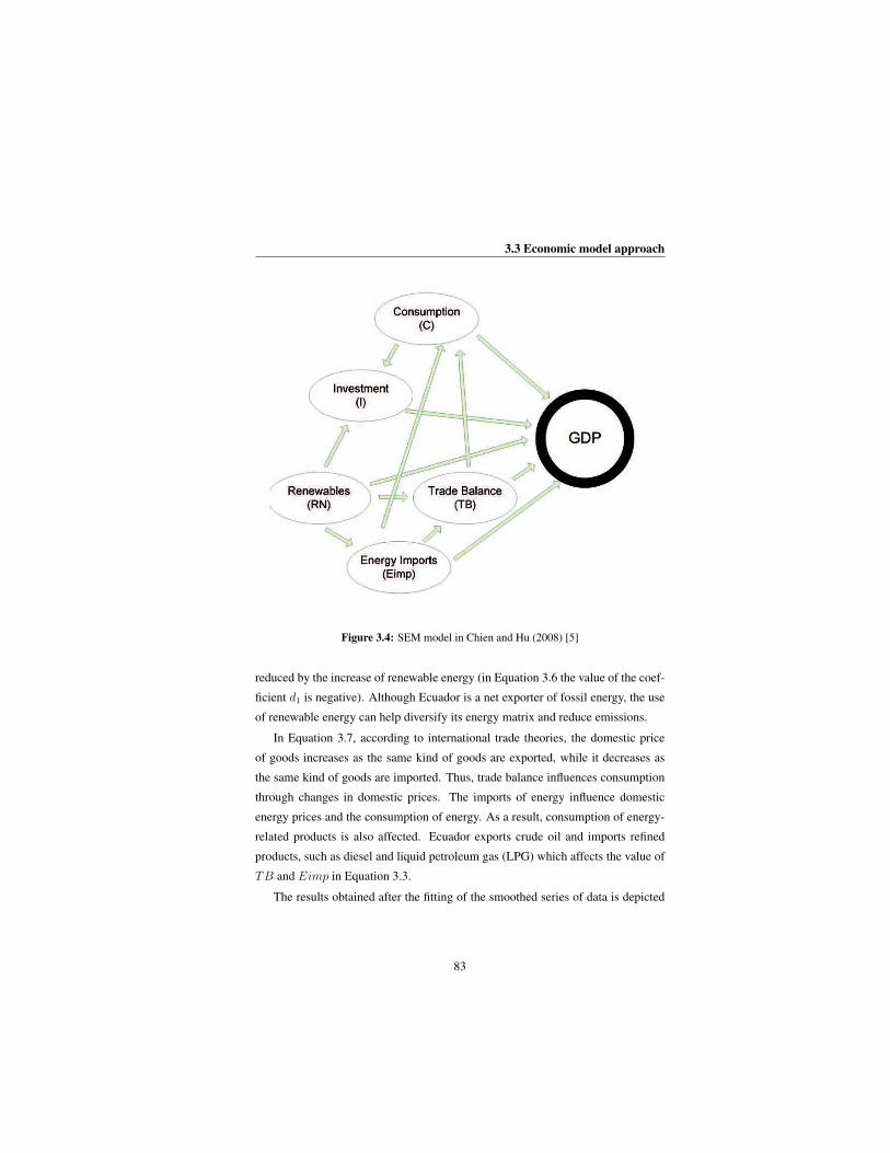
3.3 Economic model approach
Figure 3.4: SEM model in Chien and Hu (2008) [5]
reduced by the increase of renewable energy (in Equation 3.6 the value of the coef-
ficient d1 is negative). Although Ecuador is a net exporter of fossil energy, the use
of renewable energy can help diversify its energy matrix and reduce emissions.
In Equation 3.7, according to international trade theories, the domestic price
of goods increases as the same kind of goods are exported, while it decreases as
the same kind of goods are imported. Thus, trade balance influences consumption
through changes in domestic prices. The imports of energy influence domestic
energy prices and the consumption of energy. As a result, consumption of energy-
related products is also affected. Ecuador exports crude oil and imports refined
products, such as diesel and liquid petroleum gas (LPG) which affects the value of
TB and Eimp in Equation 3.3.
The results obtained after the fitting of the smoothed series of data is depicted
83

3. SYSTEM DYNAMICS MODELLING FOR RENEWABLE ENERGY
AND CO2 EMISSIONS IN ECUADOR (1980-2025)
Table 3.2: Estimated coefficients for the GDP formation equations (see Eqs. 3.3-3.7)a.
Variable GDP b I TB C Eimp
I c 1.16∗∗∗
(5.11)
-6.07∗∗∗
(-41.44)
TB d 0.99∗∗∗
(3.46)
C e 1.21∗∗∗
(7.70)
0.50∗∗∗
(100.40)
Eimpf 0.05∗∗∗
(2.66)
0.01∗∗∗
(4.14)
−0.27∗∗∗
(-100.17)
RN g −0.50∗∗∗
(-4.44)
−0.84∗∗∗
(-5.40)
0.04
(0.28)
−36.79∗∗∗
(-5.47)
a *** represents significance at the 1% level and numbers in parentheses are t-statistics.
Estimation Method: SUR. Sample: 1980-2010. Included observations: 155.
b GDP in 1010 USD.
c I in 1010 USD.
d TB in 1010 USD.
e C in 1010 USD.
f Eimp in 106 toe.
g RN in 106 toe.
in Table 3.2. Note that the error terms are correlated through the equations of
formation of GDP, because the variables in Equation 3.3 are not fully statistically
independent. All the coefficients are individually significant at the 0.01 level except
the coefficient between Eimp and TB.
According to the results of Table 3.2 renewable energy generates a reduction
on income (Q) and on invest (I) in the short term, however they have a positive
impact on the trade balance (TB) and a large negative effect on the energy imports
(Eimp).
84
3.4 Energy consumption and productive sectoral structure submodel
3.4 Energy consumption and productive sectoral struc-
ture submodel
Energy consumption refers to the use of primary energy before transformation into
any other end-use energy, which is equal to the local production of energy plus
imports and stock changes, minus the exports and the amount of fuel supplied
to ships and aircraft engaged in international transport. It is given in kt of oil
equivalent (ktoe). Energy intensity is defined as the ratio of energy consumption
and GDP [146].
The energy demand analysis starts from an analytical method that is based on
energy end use, in order to model the requirements of consumption in the different
productive sectors. Economic, demographic and energy use information applies
to build different scenarios, in order to determine how the total and disaggregated
energy sources consumption evolve over time in each industry and in each scen-
ario. The energy demand analysis is a starting point for assessing the energetic
area in integrated form, since all processing calculations and use of resources are
determined by the calculated levels of final demand.
In general, sectoral structure comprises households, industry, transport, trade,
agriculture, etc.. In turn, each sector can be divided into different sub-sectors, final
consumption and equipment that use energy. However, given the availability of
data in Ecuador, it is only possible to identify the primary energy consumption by
source and type in each of the sectors mentioned previously.
As was already mentioned in Section 2.2 in Chapter 2, the usual standard di-
vision of productive sectors follows the ISIC specification (International Standard
Industrial Classification of All Economic Activities, Rev.4), but taking in account
the availability of data, we follow the division of the productive sectors given in
Mosquera (2008) [154]: i) agriculture, fishing and mining (sec-1), ii) industry
(sec-2), iii) construction (sec-3), iv) trade and public services (sec- 4), and v)
transportation (sec-5).
Sectors will be represented inside the model by their contribution to the coun-
try’s economy (Si), by their energy intensity1 (EIi) and by their energy mix (Mij).
1Energy intensity measures the amount of energy required per unit of consumption or product,
expressed in terms of a value which is determined by the used sources which have different caloric
85
3. SYSTEM DYNAMICS MODELLING FOR RENEWABLE ENERGY
AND CO2 EMISSIONS IN ECUADOR (1980-2025)
Index i runs over each sector of the productive sectoral structure and index j runs
over each kind of fuel: i) natural gas (j = 1), ii) coal (j = 2), iii) petroleum
(j = 3), iv) renewable (j = 4), and v) alternative energy (j = 5).
3.5 CO2 intensity and energy matrix submodel
CO2 intensity (CO2int) of a given country corresponds to the ratio of CO2 emis-
sions and the total consumed energy written in terms of mass of oil equivalent.
CO2int =
∑
ij Cij∑
ij Eij
(3.8)
The value of the CO2int in a given year depends on the particular energy mix during
that year. Mij gives the energy matrix, but it is more convenient to sum over the
different sectors and aggregate the fossil fuel contributions, therefore, we define:
Mj =
∑
i Eij∑
ij Eij
(3.9)
On one hand, M1, M2, and M3 correspond to the energy consumption from natural
gas, coal, and petroleum, respectively. Therefore, the share of fossil energy in the
total consumption will be M1 + M2 + M3. On the other hand, M4 and M5 stand
for the energy consumption from renewable and alternative sources, respectively.
Therefore:
M1 +M2 +M3 +M4 +M5 = 100% (3.10)
In order to simplify the description, we assume that M4 and M5 do not contribute
to the CO2 emissions. Following the methodology recommended by the IPCC, that
is, the Reference method (IPCC, 2006) [42], the approach of the first level for the
fossil energy mix was used. The emission factors, Uij , are taken from the IPCC
methodology to estimate the CO2 emission of each fuel (IPCC, 2006) [42].
powers and by the equipment used with different technologies and efficiency levels (WB, 2012)
[146]. Note that the different economic sectors have different intensive use of energy (Cancelo,
2002) [194]. Two factors explain the differences in energy intensity between each sector: i) differ-
ences in the efficiency of the energy used in each sector and ii) differences in the economic activity
of each sector.
86
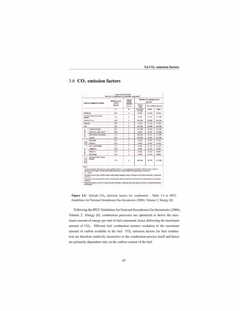
3.6 CO2 emission factors
3.6 CO2 emission factors
Figure 3.5: Default CO2 emission factors for combustion - Table 1.4 in IPCC
Guidelines for National Greenhouse Gas Inventories (2006), Volume 2: Energy [6].
Following the IPCC Guidelines for National Greenhouse Gas Inventories (2006),
Volume 2: Energy [6], combustion processes are optimized to derive the max-
imum amount of energy per unit of fuel consumed, hence delivering the maximum
amount of CO2. Efficient fuel combustion ensures oxidation of the maximum
amount of carbon available in the fuel. CO2 emission factors for fuel combus-
tion are therefore relatively insensitive to the combustion process itself and hence
are primarily dependent only on the carbon content of the fuel.
87

3. SYSTEM DYNAMICS MODELLING FOR RENEWABLE ENERGY
AND CO2 EMISSIONS IN ECUADOR (1980-2025)
The carbon content may vary considerably both among and within primary fuel
types on a per mass or per volume basis:
• For natural gas, the carbon content depends on the composition of the gas
which, in its delivered state is primarily methane, but can include small
quantities of ethane, propane, butane, and heavier hydrocarbons. Natural
gas flared at the production site will usually contain far larger amounts of
non-methane hydrocarbons. The carbon content will be correspondingly dif-
ferent.
• Carbon content per unit of energy is usually less for light refined products
such as gasoline than for heavier products such as residual fuel oil.
• For coal, carbon emissions per tonne vary considerably depending on the
coal’s composition of carbon, hydrogen, sulphur, ash, oxygen, and nitrogen.
By converting to energy units this variability is reduced. A small part of the
fuel carbon entering the combustion process escapes oxidation. This fraction is
usually small (99 to 100 percent of the carbon is oxidized) and so the default emis-
sion factors in Figure 3.5 (Table 1.4 in IPCC Guidelines for National Greenhouse
Gas Inventories (2006), Volume 2: Energy [6]) are derived on the assumption of
100 percent oxidation. For some fuels, this fraction may in practice not be negli-
gible and where representative country-specific values, based on measurements are
available, they should be used. In other words: the fraction of carbon oxidised is
assumed to be 1 in deriving default CO2 emission factors.
Figures 3.6 and 3.7 (Table 1.3 in IPCC Guidelines for National Greenhouse
Gas Inventories (2006), Volume 2: Energy [6]) give carbon contents of fuels from
which emission factors on a full molecular weight basis can be calculated (Figure
3.5). These emission factors are default values that are suggested only if country-
specific factors are not available. More detailed and up-to-date emission factors
may be available at the IPCC [6].
Note that CO2 emissions from biomass fuels are not included in the national
total but are reported as an information item, also peat is treated as a fossil fuel and
not as a biofuel and emissions from its combustion are therefore included in the
national total.
88

3.7 Model equations
Figure 3.6: Default values of carbon content - Table 1.3 in IPCC Guidelines for Na-
tional Greenhouse Gas Inventories (2006), Volume 2: Energy [6].
The data presented in Figures 3.6 and 3.7 is used to calculate default emission
factors for each fuel on a per energy basis. If activity data is available on a per mass
basis, a similar approach can be applied to these activity data directly. Obviously
the carbon content then should be known on a per mass basis.
3.7 Model equations
Below we summarize the difference equations that are used in each submodel:
89

3. SYSTEM DYNAMICS MODELLING FOR RENEWABLE ENERGY
AND CO2 EMISSIONS IN ECUADOR (1980-2025)
Figure 3.7: Default values of carbon content - Table 1.3 (Continued) in IPCC
Guidelines for National Greenhouse Gas Inventories (2006), Volume 2: Energy [6].
Q(t) = a1I(t) + a2TB(t) + a3C(t) + a4Eimp(t) + a5RN(t−1), (3.11)
Ej(t) =∑
i
Si(t) · EIi(t) ·Mij(t) ·GDP(t), (3.12)
RN(t) = E4(t) + E5(t), (3.13)
y(t) = y(t−1) · (1 + ry), (3.14)
where Si(t), EIi(t), Mij(t), I(t), TB(t), C(t), and Eimp(t) evolve following Equation
3.14 while the parameters ai have constant values. Note that index j runs over
the type of energy sources, while i on the industrial sectors; j = 4 and j = 5
corresponds to renewable and alternative energy, respectively. t = 0 corresponds
90

3.8 Causal diagram of CO2 emissions
to the base year and t is given in number of years since 1980. The value of ry is
fixed through the definition of the used scenario,
ry =
(
y(tf)y(0)
)1/tf
− 1, (3.15)
where tf is the future time for which we establish the goal (y(tf)), and y0 is the
starting value of the function. According to Rowland (2003) [179] and Jin et al.,
[180], to extrapolate the trend of the period 1980-2010 in the base scenario (trend),
one should use a value of ry that depends on the time,
ry(t) =
(
y(t−1)
y(t−n)
)1/n
− 1, (3.16)
where n is the number of years of the dataset period, i.e., 30 in our case. The feed-
back mechanism is provided through the inclusion of RN(t−1) in the calculation of
the income (Q) (Equation 3.11). As a5 < 0 (see Table 3.2) the feedback mechan-
ism is negative. This fact induces a decrease of the GDP for the SC-3 and SC-4
scenarios with respect to SC-2 (see section 3.10.1 in this Chapter) for increasing of
renewable energy use. In general, any increase of the terms∑
i Si(t) ·EIi(t) ·Mij(t)
for j = 4 and j = 5 will induce a reduction, though moderate, of the income.
In Figure 3.8 we present the schematic view of the whole model. It is worth
noting the feedback mechanism between renewable energy and GDP. This is one
of the keys of the model, which allows us to generate a non-trivial evolution of
the system. In this Figure, we can identify the economic submodel, the energy
consumption and productive sectoral submodel, as well as the CO2 intensity and
energy matrix submodel.
3.8 Causal diagram of CO2 emissions
To understand why and how CO2 emissions change over time, we need to know
the factors that separately affect or control CO2 emissions. In particular, it is ex-
tremely useful to represent the driving forces of CO2 emissions in a hierarchical
way, showing the causality relationship between the different variables. All this
information constitutes the causal diagram. In this work the variables that will de-
termine the amount of CO2 emissions are: GDP (formation components), share of
91
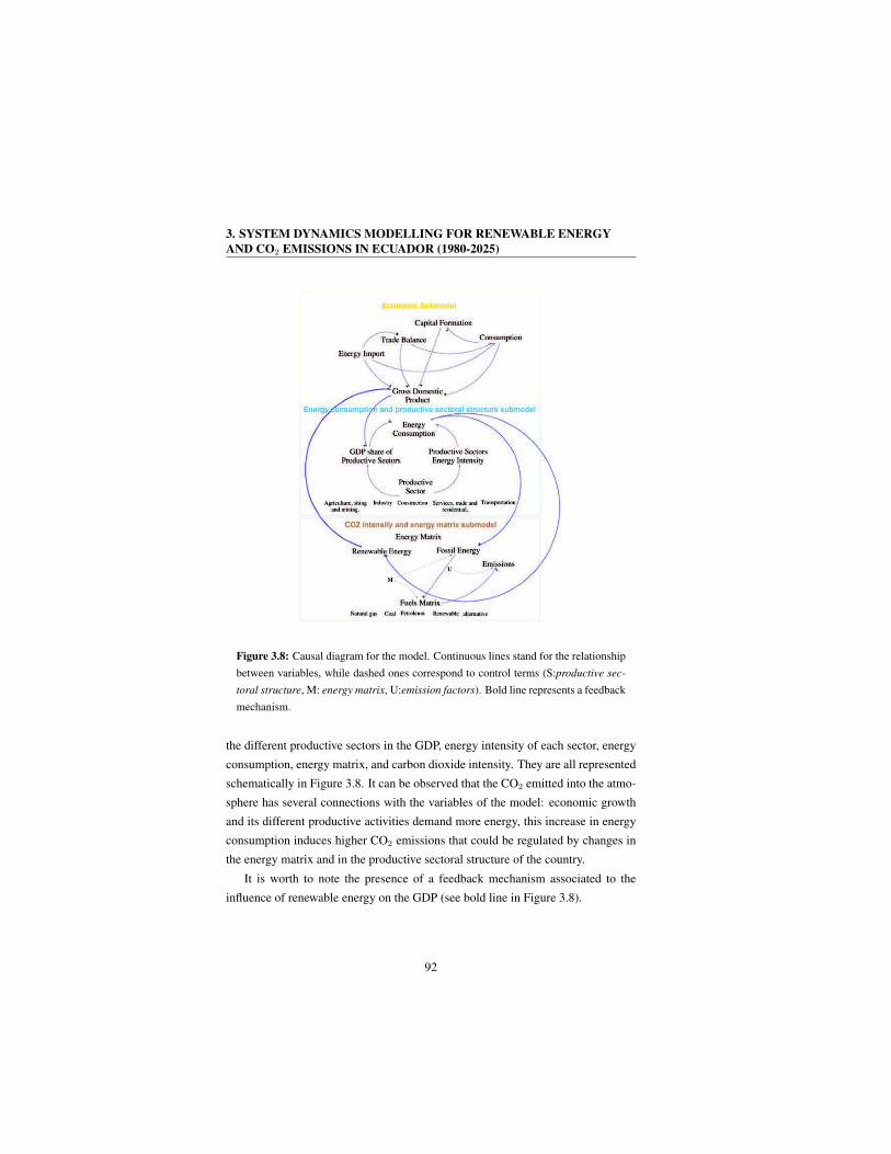
3. SYSTEM DYNAMICS MODELLING FOR RENEWABLE ENERGY
AND CO2 EMISSIONS IN ECUADOR (1980-2025)
Figure 3.8: Causal diagram for the model. Continuous lines stand for the relationship
between variables, while dashed ones correspond to control terms (S:productive sec-
toral structure, M: energy matrix, U:emission factors). Bold line represents a feedback
mechanism.
the different productive sectors in the GDP, energy intensity of each sector, energy
consumption, energy matrix, and carbon dioxide intensity. They are all represented
schematically in Figure 3.8. It can be observed that the CO2 emitted into the atmo-
sphere has several connections with the variables of the model: economic growth
and its different productive activities demand more energy, this increase in energy
consumption induces higher CO2 emissions that could be regulated by changes in
the energy matrix and in the productive sectoral structure of the country.
It is worth to note the presence of a feedback mechanism associated to the
influence of renewable energy on the GDP (see bold line in Figure 3.8).
92

3.9 Model validation and verification
3.9 Model validation and verification
Figure 3.9: Left: Comparative of model result vs. historical data. Right: Time series
of MAPE term at time t, see Ecuation 3.17.
Official dataset from 1980 to 2010 and the output of the model for the same
period can be compared to test the reliability and robustness of the model. This
analysis can be carried out calculating the mean absolute percentage error (MAPE)
that is a measure of accuracy of a method for constructing fitted time series val-
ues in statistics, specifically in trend estimation. MAPE is most commonly used
to evaluate cross-sectional forecasts (Ahlburg, 1995 [195]; Campbell, 2002 [196];
Hyndman and Koehler, 2006 [197]; Isserman, 1977 [198]; Miller, 2001 [199]; Mur-
dock et al., 1984 [200]; Rayer, 2007 [201]; Sink, 1997 [202]; Smith, 1987 [203];
93
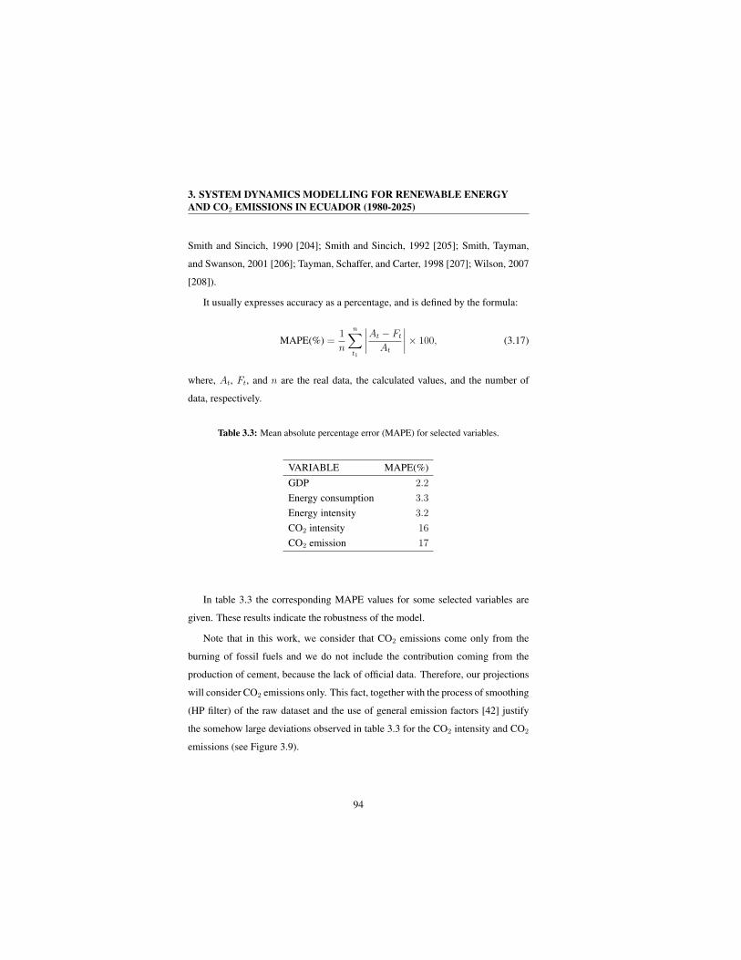
3. SYSTEM DYNAMICS MODELLING FOR RENEWABLE ENERGY
AND CO2 EMISSIONS IN ECUADOR (1980-2025)
Smith and Sincich, 1990 [204]; Smith and Sincich, 1992 [205]; Smith, Tayman,
and Swanson, 2001 [206]; Tayman, Schaffer, and Carter, 1998 [207]; Wilson, 2007
[208]).
It usually expresses accuracy as a percentage, and is defined by the formula:
MAPE(%) =1
n
n∑
t1
∣
∣
∣
∣
At − Ft
At
∣
∣
∣
∣
× 100, (3.17)
where, At, Ft, and n are the real data, the calculated values, and the number of
data, respectively.
Table 3.3: Mean absolute percentage error (MAPE) for selected variables.
VARIABLE MAPE(%)
GDP 2.2
Energy consumption 3.3
Energy intensity 3.2
CO2 intensity 16
CO2 emission 17
In table 3.3 the corresponding MAPE values for some selected variables are
given. These results indicate the robustness of the model.
Note that in this work, we consider that CO2 emissions come only from the
burning of fossil fuels and we do not include the contribution coming from the
production of cement, because the lack of official data. Therefore, our projections
will consider CO2 emissions only. This fact, together with the process of smoothing
(HP filter) of the raw dataset and the use of general emission factors [42] justify
the somehow large deviations observed in table 3.3 for the CO2 intensity and CO2
emissions (see Figure 3.9).
94

3.10 Scenarios
3.10 Scenarios
3.10.1 Scenario analysis for income, energy and emissions
As mentioned in Section 1.7 in Chapter 1, scenario analysis is used in a wide range
of purposes in the literature. The primary function of the scenario approach in
economy growth, energy consumption and emission in this research is to respond
to uncertainty and potentially to develop strategic insights for policy.
Sometimes the terminology used to describe possible future conditions in the
context of income, energy and emissions is often interchangeable in the literat-
ure. Holmes (2007) [209] notes some important distinctions. Whereas projections,
forward historical data or past trends and forecasts, all of them are predictive and
seek to determine the most likely future, scenarios look at diverging trends and the
potential unfolding of new dynamics.
Rather than prediction, scenario approach seeks to describe a spectrum of pos-
sibilities. This is a bounded package of probability that could cover the range of
plausible outcomes. Economic and environmental scenarios are used in contexts
where dynamic complex systems are subject to uncertainties.
These uncertainties include inadequate scientific understanding, data gaps and
inherent uncertainties on future events (Nakicenovic, 2000) [64]. Sometimes fore-
casts and projections are based on producing Business As Usual (BAU) or central
best guess estimates and the high/low or optimistic/pessimistic variants of these.
According to Nakicenovic (2000) [64], the formulation of a range of emis-
sion scenarios is an appropriate technique to encompass uncertainties and deliver
policy insights. With the use of scenario approach, some concern of decision-
makers about the quantitative point forecasts of single most likely estimates arises.
While this can reflect an ease of understanding of single estimates, or simply what
decision-makers are accustomed to, these forecasts can also reflect a particular set
of values or interests promoted as objective information. This concern with fore-
casts may not be appropriate to either scientific inquiry or to strategic thinking in
decision-making, but it is a practice issue for scenarios.
Nielsen and Karlsson (2007) [40] note a science-policy nexus issue as techno-
logical and economic rationalities are implicitly embedded in models. This opens
95
3. SYSTEM DYNAMICS MODELLING FOR RENEWABLE ENERGY
AND CO2 EMISSIONS IN ECUADOR (1980-2025)
the question of the worldview, values and philosophy underpinning supposedly ob-
jective scientific information. This information can reflect specific futures that are
profitable or preferable to certain interests or can be used to legitimise results rather
than guide policy. The use of scenarios offers an approach to make world views
more explicit, through the description of underlying themes in narratives. It can
also be used to document assumptions used in modelling.
3.10.2 Proposal of scenarios for Ecuador 2010-2025
The goals that will be considered to define the different scenarios that will be pro-
posed, under the general purpose of improve the quality of life of people with the
least environmental impact are:
• Goal 1, by 2025 the GDP per capita will reach the international average (≈
15000 USD according to our estimates based on World Bank data) through
a process of industrialization and improvement of the productive sectoral
structure of the country;
• Goal 2, in regard to the Goal 1, the use of renewable energy will be increased
up to almost 30% of the total energy consumption;
• Goal 3, in regard to Goal 1 and Goal 2, the energy efficiency will be enlarged
by a reduction of the energy intensity and by changes in the productive sec-
toral structure.
Taking into account the latter goals, we propose four scenarios concerning the
growth of the income, the evolution of the energy matrix and of the productive
sectoral structure for the period 2011-2025.
1. Baseline scenario (BS): the GDP, the energy matrix and the productive sec-
toral structure will evolve through the smooth trend of the period 1980-2010
extrapolated to 2011-2025 using the geometric growth rate method.
2. Increasing GDP scenario (SC-2): GDP will increase approximately up to
be double of reference GDP (2010) by 2025. To generate this scenario a
constant annual growth of GDP formation components (I , TB, C, Eimp,
96

3.10 Scenarios
see Section 3.3.3 in this Chapter) of 7% per year between 2011 to 2025 will
be assumed and a structural change in the productive sectoral structure will
be implemented through a growth of 1% per year in the GDP share (Si) in the
sectors with more profit in the country economy: industry sector (sec-2) and
trade and public service sector (sec-4). The rest of the variables will evolve
as in the BS scenario. This scenario clearly corresponds to a situation where
the economy is growing rapidly and no mitigation measurements to reduce
the CO2 emissions are carried out.
3. Increasing GDP and share of renewable energies scenario (SC-3): increas-
ing GDP and change in productive sectoral structure as in the SC-2 scenario
is considered, however the share of fossil energy, will be reduced approxim-
ately one point per year, passing from a 88% in 2011 to 67% in 2025 due to a
constant annual growth of share in renewable and alternative energy (M4 and
M5). This scenario shows a first measure of environmental responsibility in
order to try to reduce dependence of fossil energy.
4. Increasing GDP and share of renewable energies and improvement in energy
efficiency scenario (SC-4): increasing GDP, change in productive sectoral
structure and change in share of fossil energy as in SC-3 scenario is carried
out. Moreover, an improvement in energy efficiency is implemented with a
1% reduction of energy intensity in industry sector (sec-2), in trade and pub-
lic services sector (sec-4) and in transportation sector (sec-5). This scenario
takes a step towards improving the country’s environmental responsibility
and sustainable development by supporting their energetic saving measures
and energy efficiency.
Both SC-3 and SC-4 scenarios goals are realistic considering the state of devel-
opment and evolution of energy technology in various energy projects implemented
by the Ecuadorian government, and the trends in the use of renewable energies in
the country [154] (see Section 2.5 and Section 2.6 in Chapter 2 ).
97
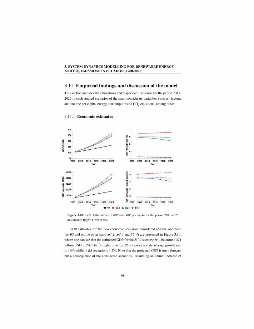
3. SYSTEM DYNAMICS MODELLING FOR RENEWABLE ENERGY
AND CO2 EMISSIONS IN ECUADOR (1980-2025)
3.11 Empirical findings and discussion of the model
This section includes the estimations and respective discussion for the period 2011-
2025 in each studied scenarios of the main considerate variables, such as: income
and income per capita, energy consumption and CO2 emissions, among others.
3.11.1 Economic estimates
Figure 3.10: Left: Estimation of GDP and GDP per capita for the period 2011-2025
in Ecuador. Right: Growth rate.
GDP estimates for the two economic scenarios considered (on the one hand
the BS and on the other hand SC-2, SC-3 and SC-4) are presented in Figure 3.10,
where one can see that the estimated GDP for the SC-2 scenario will be around 271
billion USD in 2025 (61% higher than for BS scenario) and its average growth rate
is 6.6% while in BS scenario is 3.2%. Note that the projected GDP is not a forecast
but a consequence of the considered scenarios. Assuming an annual increase of
98
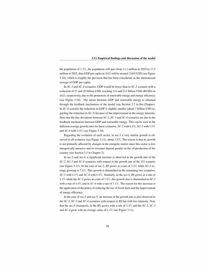
3.11 Empirical findings and discussion of the model
the population of 1.2%, the population will pass from 14.5 million in 2010 to 17.6
million in 2025, thus GDP per capita in 2025 will be around 15000 USD (see Figure
3.10), which is roughly the prevision that has been considerate as the international
average of GDP per capita.
In SC-3 and SC-4 scenarios, GDP would be lower than in SC-2 scenario with a
reduction of 27 and 20 billion USD, reaching 244 and 251 billion USD (BUSD) in
2025, respectively, due to the promotion of renewable energy and energy efficiency
(see Figure 3.10). The nexus between GDP and renewable energy is obtained
through the feedback mechanism of the model (see Section 3.7 in this Chapter).
In SC-4 scenario the reduction in GDP is slightly smaller (about 7 billion USD re-
garding the reduction in SC-3) because of the improvement in the energy intensity.
Note that the tiny deviations between SC-2, SC-3 and SC-4 scenarios are due to the
feedback mechanism between GDP and renewable energy. This can be seen in the
different average growth rates for these scenarios, SC-2 with 6.6%, SC-3 with 5.8%
and SC-4 with 6.0% (see Figure 3.10).
Regarding the evolution of each sector, in sec-1 a very similar growth is ob-
served in all scenarios (see Figure 3.11), about 3.8%. The reason is that its growth
is not primarily affected by changes in the energetic matrix since this sector is less
energetically intensive and its revenues depend greatly on the oil production of the
country (see Section 2.2 in Chapter 2).
In sec-2 and sec-4, a significant increase is observed in the growth rate of the
SC-2, SC-3 and SC-4 scenarios with respect to the growth rate of the BS scenario
(see Figure 3.11). In the case of sec-2, BS grows at a rate of 3.3% while SC-2 av-
erage growing is 7.6%. This growth is diminished in the remaining two scenarios,
SC-3 with 6.5% and SC-4 with 6.9%. Similarly, in the sec-4, BS grows at a rate of
2.4% while the SC-2 grows at a rate of 7.6%, this growth also is diminished in SC-3
with a rate of 6.9% and in SC-4 with a rate of 7.1%. The reason for this decrease is
the application of the policy of reducing the use of fossil fuels and the improvement
of energy efficiency.
In the case of sec-3 and sec-5, an increase in the growth rate is also observed in
the SC-2, SC-3 and SC-4 scenarios with respect to BS but with less intensity. Note
that the sec-5 (transport), in the BS, grows with a rate of 3.4% and the SC-2, SC-3
and SC-4 grow with an average value of 6.4% (see Figure 3.11).
99

3. SYSTEM DYNAMICS MODELLING FOR RENEWABLE ENERGY
AND CO2 EMISSIONS IN ECUADOR (1980-2025)
Figure 3.11: Left: Estimation of GDP by sector for the period 2011-2025 in Ecuador.
Right: Growth rate.
Figure 3.12 shows the estimation of the Productive Sectorial Matrix (PSM) for
the BS and for the alternative scenarios (SC-2, SC-3 and SC-4). In BS case, we can
observe that the largest sector is sec-1 (includes income from petroleum) that rep-
resented around 34% of GDP in the period 2011-2025, reinforcing the country’s oil
dependence, followed by sec-4 (31%), sec-2 (14%), sec-3 (11%) and sec-5 (10%).
In the alternative scenarios, we can observe a change in the shares of PSM and
Sec-4 is now the largest sector (35%), following by sec-1 but with a less share that
in previous case (28%), sec-2 (industry) growth up to 16%, sec-3 (11%) and sec-5
(10%). Note that the share of sec-5 (transportation) keeps constant.
100

3.11 Empirical findings and discussion of the model
Figure 3.12: Estimation of Productive Sectorial Matrix in Ecuador 2011-2025.
3.11.2 Energy estimates
Energy consumption is calculated through the product of the energy intensity of
each productive sector (EIi) and the corresponding share of the GDP (Qi) of every
sector. The values of the energy consumption for the period 2011-2025 are repres-
ented in Figure 3.13. In 2025 the BS scenario generates a consumption of 20520
ktoe, the SC-2 scenario about 36040 ktoe (76% higher than the BS scenario), and
the SC-3 scenario generates a consumption of 32425 ktoe (58% higher than the BS
scenario). These two last scenarios show the growth of the energy consumption
due to the increase of GDP and to the changes of the productive sectoral structure.
Finally, SC-4 scenario generates a consumption of 26740 ktoe (only 30% higher
than in the BS scenario). It clearly shows the benefits of the reduction of the energy
intensity.
In Figure 3.13, we can see that there are three pathways followed by the dif-
ferent proposed scenarios, the most energetically intensive is the path followed by
101

3. SYSTEM DYNAMICS MODELLING FOR RENEWABLE ENERGY
AND CO2 EMISSIONS IN ECUADOR (1980-2025)
Figure 3.13: Lefth: Estimation of energy consumption and energy intensity for the
period 2011-2020 in Ecuador. Right: Growth rate.
SC-2 and SC-3 (indistinguishable in the used scale) , due to its larger energy con-
sumption and low energy efficiency goal. Indeed, in these scenarios the energy
intensity increases more than 15% (period 2011-2025). The path taken by SC-4 is
clearly the most energetically efficient, with a reduction of 6% in energy efficiency,
while BS follow the trend path with a increase of 7% in the whole period.
The estimated values of energy intensity and energy consumption in each pro-
ductive sector till 2025 are shown in Figure 3.14 and Figure 3.15, respectively to
illustrate the differences between sectors. In Figure 3.14, one can clearly see the
results of the implementation of energy efficiency goals set for each sector (es-
pecially for sec-2, sec-4 and sec-5) in scenario SC-4 (see Section 3.10.2 in this
Chapter). Indeed, sec-5 in SC-4 scenario has a reduction in its energy intensity
value of almost 165 points (ktoe/BUSD) respect to the value in the rest of scenarios
102
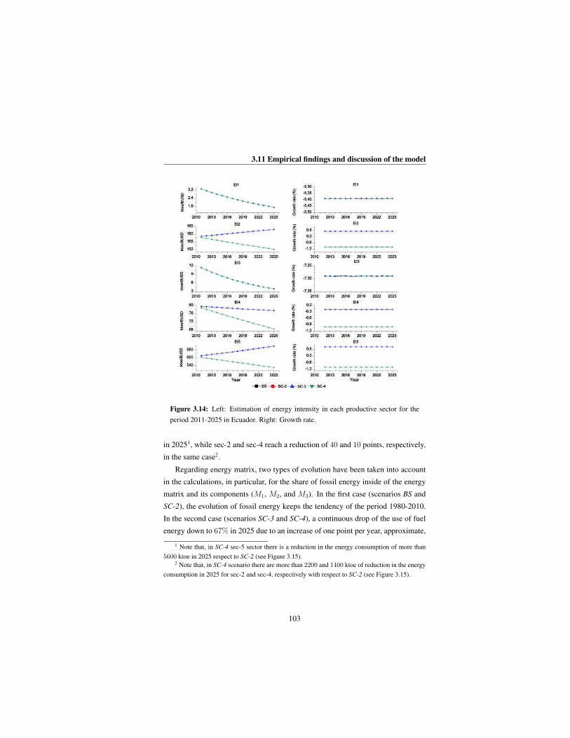
3.11 Empirical findings and discussion of the model
Figure 3.14: Left: Estimation of energy intensity in each productive sector for the
period 2011-2025 in Ecuador. Right: Growth rate.
in 20251, while sec-2 and sec-4 reach a reduction of 40 and 10 points, respectively,
in the same case2.
Regarding energy matrix, two types of evolution have been taken into account
in the calculations, in particular, for the share of fossil energy inside of the energy
matrix and its components (M1, M2, and M3). In the first case (scenarios BS and
SC-2), the evolution of fossil energy keeps the tendency of the period 1980-2010.
In the second case (scenarios SC-3 and SC-4), a continuous drop of the use of fuel
energy down to 67% in 2025 due to an increase of one point per year, approximate,
1 Note that, in SC-4 sec-5 sector there is a reduction in the energy consumption of more than
5600 ktoe in 2025 respect to SC-2 (see Figure 3.15).2 Note that, in SC-4 scenario there are more than 2200 and 1400 ktoe of reduction in the energy
consumption in 2025 for sec-2 and sec-4, respectively with respect to SC-2 (see Figure 3.15).
103
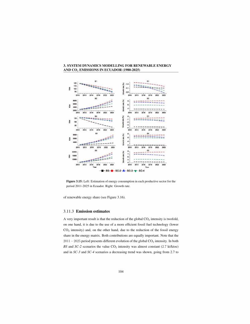
3. SYSTEM DYNAMICS MODELLING FOR RENEWABLE ENERGY
AND CO2 EMISSIONS IN ECUADOR (1980-2025)
Figure 3.15: Left: Estimation of energy consumption in each productive sector for the
period 2011-2025 in Ecuador. Right: Growth rate.
of renewable energy share (see Figure 3.16).
3.11.3 Emission estimates
A very important result is that the reduction of the global CO2 intensity is twofold,
on one hand, it is due to the use of a more efficient fossil fuel technology (lower
CO2 intensity) and, on the other hand, due to the reduction of the fossil energy
share in the energy matrix. Both contributions are equally important. Note that the
2011−2025 period presents different evolution of the global CO2 intensity. In both
BS and SC-2 scenarios the value CO2 intensity was almost constant (2.7 kt/ktoe)
and in SC-3 and SC-4 scenarios a decreasing trend was shown, going from 2.7 to
104

3.11 Empirical findings and discussion of the model
Figure 3.16: Estimation of energy matrix for the period 2011-2025 in Ecuador.
2.1 kt/ktoe between 2011 and 2025 (see Figure 3.17).
Figure 3.17 shows CO2 emissions as a function of time for the period 2011-
2025, under the four considered scenarios. In 2025 the highest CO2 emission cor-
responds to the SC-2 scenario, while the lowest corresponds to the SC-4 scenario.
The SC-3 and SC-4 scenarios, which imply the continuous growth of the GDP and
the application of attenuation measures, with a reduction of the fossil energy contri-
bution to the energy matrix and changes in the productive sectoral structure, present
a clear reduction of CO2 emissions with respect to the SC-2 scenario. In particular,
in 2025 CO2 emissions would reach 97 thousand kt in SC-2 scenario, and only 55
thousand kt in BS scenario. With the reduction of fossil energy, down to 67% in
SC-3 scenario, without modifying the energy intensity, one reaches 66 thousand kt,
while implementing energy efficiency measures in the productive sectoral structure
(SC-4 scenario) emissions are reduced down to 54 thousand kt.
The BS scenario presents CO2 emissions in 2025, 1.7 times higher than in 2010,
while the SC-2 scenario gives rise to an increase of 2.8 times. This implies that the
amount of CO2 emissions in the SC-2 scenario during the period 2011-2020 will
105
3. SYSTEM DYNAMICS MODELLING FOR RENEWABLE ENERGY
AND CO2 EMISSIONS IN ECUADOR (1980-2025)
Figure 3.17: Left: Estimation of CO2 and CO2 intensity for the period 2011-2025 in
Ecuador. Right: Growth rate.
be 260 thousand kt higher than in the BS scenario. Scenarios where renewable
energy and efficiency goals are implemented show that it is possible to increase the
GDP in a constant way, mitigating, at the same time, the CO2 emissions, therefore
reducing the rise of the emissions due to the higher economic activity. In particular,
the most efficient scenario, SC-4, presents a remarkable reduction. In 2025 CO2
emissions will be 43% lower than in the SC-2 scenario. Furthermore, the SC-3
scenario generates 115 thousand kt more than BS scenario during the 2011-2025
period, which supposes a reduction of 30 thousand kt with respect to SC-2 scenario.
Finally, the SC-4 scenario generates 300 kt less than BS scenario during the same
period, which supposes a large reduction of 41 thousand kt with respect to the SC-2
scenario.
The estimated values of CO2 intensity and CO2 emissions in each productive
sector till 2025 are shown in Figure 3.18 and Figure 3.19 respectively to illustrate
the differences between sectors. In Figure 3.18, we can see the results of the im-
106

3.11 Empirical findings and discussion of the model
Figure 3.18: Left: Estimation of CO2 intensity in each productive sector for the period
2011-2025 in Ecuador. Right: Growth rate.
plementation of green goals set for each sector (especially for sec-2 and sec-5) in
scenario SC-4 (see Section 3.10.2 in this Chapter). Indeed, sec-5 in SC-4 scenario
presents a reduction in its CO2 intensity value of 55, 220 and 95 points (kt/ktoe)
respect to the value of BS, SC-2 and SC-3 in 2025, respectively. Note that, in SC-4
scenario there are more than 4, 24 and 7 thousand kt of reduction in emissions of
transport sector (sec-5) in 2025 respect to BS, SC-2 and SC-3 scenarios, respect-
ively (see Figure 3.19). While sec-2 in SC-4 reach a reduction of 88 and 136 points
with respect to SC-2 and SC-3, respectively, and only has 4 point more than the
value of CO2 intensity in BS scenario. Note that, in SC-4 scenario there are almost
10 and 3 thousand kt of reduction in emissions of industry sector (sec-2) in 2025 re-
spect to SC-2 and SC-3, respectively, and only 600 kt more than in the BS scenario
107

3. SYSTEM DYNAMICS MODELLING FOR RENEWABLE ENERGY
AND CO2 EMISSIONS IN ECUADOR (1980-2025)
Figure 3.19: Left: Estimation of CO2 in each productive sector for the period 2011-
2025 in Ecuador. Right: Growth rate.
(see Figure 3.19).
3.12 Summary and conclusions of the chapter
This Chapter presents a model based on a variation of the Kaya Identity and on an
approach of GDP formation which is supported with the use of renewable energy.
The official data set (1980-2010) was used to parameterize the model, while with
the second part of the period (2011-2025) an estimation of different variables, in-
cluding the CO2 emissions, was carried out. To this end, the GDP and the energy
intensity have been modeled. Moreover, different scenarios that present the evolu-
tion of the energy matrix and the productive sectoral structure have been defined.
108
3.12 Summary and conclusions of the chapter
First, a BS scenario (baseline scenario) has been defined, in which the vari-
ables of the model were parameterized according to the observed tendency during
the period 1980-2010, assuming a geometric growth rate during the period 2011-
2025. The second scenario, called SC-2, is characterized by the increasing (relative
to 2010) of the GDP during the period 2011-2025 (with the goal of reaching the
estimated international average GDP per capita in 2025). In the third scenario,
called SC-3 scenario, besides assuming the increasing of the GDP, we impose the
decreasing of the fossil energy share (ES1) up to 67%. Finally, in the fourth one,
SC-4 scenario, we complement the SC-3 scenario including changes in the product-
ive sectoral structure to achieve a reduction of energy intensity, which supposes a
lower CO2 intensity.
The main outcome of this chapter are the estimates of CO2 emissions by the
period 2011-2025 in each scenario (see Section 3.11.3 in this Chapter). By 2025
the BS scenario reaches 55 thousand kt, in the SC-2 scenario it corresponds to 97
thousand kt, in SC-3 scenario to 66 thousand kt, and in the SC-4 scenario to 55
thousand kt of CO2. Note that the BS scenario corresponds to a modest GDP in-
crease, while in the others the GDP increases heavily. The highest emissions are
for the SC-2 scenario where no mitigation measures are taken. The other two scen-
arios show us that it is possible a sizable reduction of the emissions, promoting
the renewable energy (SC-3 scenario) and on top of that modifying the productive
sectoral structure, therefore, reducing the energy and the CO2 intensities, as in the
SC-4 scenario. It is worth to note that both promotion of renewable energy and im-
provement of the energy intensity are equally effective attenuating CO2 emissions.
109

Adapt or perish, now as ever, is
nature’s inexorable imperative.
H. G. Wells
CHAPTER
4Decomposition analysis in
income and energy
consumption related with
CO2 emissions in Ecuador
(1980-2025)
4.1 Overview
In the present chapter, we discuss the decomposition analysis (DA) methodology
applied within this research. This section presents the used technique, the applied
mathematical methodology and the construction of an appropriate identity to meas-
ure the change of CO2 emission in Ecuador during the period 1980-2025. Change
is measured at both macro and disaggregated sectoral level. Specific aspects related
to the application of DA to both the historical period (1980-2010) and in medium
term prevision (2011-2025) for the proposed scenarios are discussed.
DA is widely applied in understanding changes in economic, energy consump-
tion, environmental, employment and other socio-economic indicators (Hoekstra
111
4. DECOMPOSITION ANALYSIS IN INCOME AND ENERGY
CONSUMPTION RELATED WITH CO2 EMISSIONS IN ECUADOR
(1980-2025)
and van den Bergh, 2003) [210]. Several DA methodologies have been developed
specifically to analyze changes in energy and emissions. Two main streams of
inquiry have evolved under the concept of DA: i) Index Decomposition Analysis
(IDA) and i) Structural Decomposition Analysis (SDA).
These techniques have been used for both temporal and cross country/region
analysis. IDA is formulated using concepts similar to the index numbers used in
economics and statistics. This technique is more popular in the literature than SDA
which is based on an input-output model (Ang, 2004a) [211]. At first sight, the
advantages of IDA over SDA include the requirement for less data (Hatzigeorgiou
et al., 2008) [212]. In IDA, absolute, structural and elasticity indicators have been
analysed in contrast to SDA which has generally been restricted to absolute indic-
ators. In many countries input-output tables are not constructed annually. IDA
also permits the exploration of a share effect in industry or transport, indeed, this
methodology has a great development and application studies in the literature. In
contrast, SDA can distinguish between technological and demand effects which is
not possible in IDA. Zhou and Ang, (2008) [213] propose that IDA is more flexible
for aggregate data studies, Hatzigeorgiou (2008) [212] points the requirement for
less data and the use of three indicator forms as comparative advantages of IDA
approach, while Ang (2004a) [211] states its simplicity and flexibility.
Since late 1970s IDA methods have undergone several deep changes in scope
of application. The reason is the expanding from applications in industry to energy
demand and emission analysis across various sectors. Key to the application of
IDA is the decomposition of change as an indicator, using a governing function to
a number of predefined factors of interest to the analysis (Zhou, 2008) [213]. This
idea can be used to get insight into the effect of the driving forces1 or determinants
that underlie changes. IDA approach is now a widely accepted analytical tool for
energy and carbon emissions analysis (Ang, 2004) [52]. The technique has direct
policy implications as it can be used to accurately quantify effects including eval-
uation of energy conservation programs and the outcome may provide a basis for
1In DA, the driving forces are determined by the governing function designed and are quant-
itative. In scenario analysis, driving forces can potentially overlap with those described by the
DA approach, but they also encompass qualitative aspects that sometimes cannot be captured by
modelling.
112
4.2 Decomposition techniques in explanatory factors. Aggregate data
decomposition
forecasting (Ang, 2004a) [211].
4.2 Decomposition techniques in explanatory factors.
Aggregate data decomposition
Proops et al (1993) [214] decompose the growth rate of CO2 emissions considering
an aggregate economic activity, that is, without taking into account the relative
weights of the different productive sectors. They identified three variables that
influence the temporal evolution of CO2 emissions, which are:
• The ratio of CO2(C) and energy used (E): CE
,
• The ratio of energy used in the economy (E) and the GDP (Q): EQ
,
• The GDP of the economy (Q).
These variables are related in the following identity:
C =
(
C
E
)(
E
Q
)
Q. (4.1)
Taking logarithms of the identity 4.1 and differentiating1 respect to time:
C ′
C=
(
(C/E)′
C/E
)
+
(
(E/Q)′
E/Q
)
+Q′
Q. (4.2)
Considering that time series are in discrete time and taking into account that x′ =dxdt
≈ ∆x∆t
and assuming that ∆t = 1, then x′
x≈ ∆x
x, Equation 4.2 can be approached
as,∆C
C≈
∆(C/E)
C/E+
∆(E/Q)
E/Q+
∆Q
Q. (4.3)
As Equation 4.3 is a discrete approximation, the result in both sides of the equation
do not match and always will exist a residue.
Therefore, according to equation 4.3, the variation of CO2 will be influenced
by the following variables:
1Wherein the ′ represents the first derivative with respect to time, x′ = dxdt .
113
4. DECOMPOSITION ANALYSIS IN INCOME AND ENERGY
CONSUMPTION RELATED WITH CO2 EMISSIONS IN ECUADOR
(1980-2025)
• The variation of the ratio CE
: this variation would be picking the modification
of the fuel mix, so as to provide the same amount of energy a different quant-
ity of CO2 is emitted. Another possibility is that technologies that reduce
emissions at the end of the process are applied.
• The variation of the ratio EQ
: it is the modification of the energy requirements
to produce one unit of GDP. The variation of the ratio EQ
could take place
either because it increases the efficiency of energy production or because the
structure is modified to sectors with lower energy requirements.
• The variation of Q: is the change in the GDP of the economy.
If we consider the three effects of first level mentioned in Grossman and Krueger
(1991) [131] (effect scale, composition and technology, see Section 5.2.2 in Chapter
4), CO2 change in Equation 4.3 can be explained through tree terms: i) the first is
the technological effect, ii) the second refer to the rest of the technological effect
(related to the improved efficiency in the use of resources), and the composition
effect, iii) the third is the scale effect. Although Proops et al (1993) [214] pro-
posed this decomposition to be used for CO2, it could be used for any contaminant
associated with energy use.
This decomposition, some times called aggregate data decomposition, pre-
cisely because it does not incorporate information neither on the behavior of the
different sectors nor introduce specific information on the fuel mix used, this ap-
proach represent the economic system as a whole. Since we need to incorporate
information about productive sectors and energy mix to understand their behavior
and effect on emission (disaggregated data) and because this will introduce a sum
term inside Equation 4.3, a new approach is needed.
4.3 Index decomposition analysis (IDA)
These methods began to be used to decompose the energy consumption and energy
intensity but later extended its use to the decomposition of pollutant emissions
related to energy (notably CO2, SO2 and NOx).
114
4.3 Index decomposition analysis (IDA)
According to Ang and Zhang (2000) [55], the two most used IDA methods in
the literature have been the Laspeyres and arithmetic mean Divisia index. Follow-
ing Ang and Zhang (2000) [55] and Ang (1994) [215], we choose as an indicator
the energy intensity of the industry, to shorten the explanation, since it involves
only two factors decomposition whereas if we decompose, e.g., emissions related
to energy, we have to work with four factors. Also, we will introduce some refer-
ence to the decomposition of CO2 emissions that will be used in the case of study
in Section 4.5 in this Chapter.
We define the following variables for year t:
• Et: total energy consumption in the industry.
• Eit: energy consumption in the industrial sector i.
• Yt: total industry output.
• Yit: production of industrial sector i.
• Sit: share of the industrial sector i (Yit/Yt).
• It: aggregate energy intensity (Et/Yt).
• Iit: energy intensity of sector i (Eit/Yit).
The aggregate energy intensity can be expressed as:
It =∑
i
SitIit, (4.4)
where the sum is taken over all industrial sectors (i). In Equation 4.4 the aggregate
energy intensity is expressed in terms of the production structure and the sectoral
energy intensities.
To analyze the variation of It as a funtion of changes of its components, i.e., Sit
and Iit, we will differentiate Equation 4.4 with respect to time,
I ′t =∑
i
(IitS′
it + I ′itSit) . (4.5)
Following Ang and Zhang (2000) [55], if we assume that the aggregate energy
intensity varies from I0 at time 0 to IT at time T , this change can be expressed
115

4. DECOMPOSITION ANALYSIS IN INCOME AND ENERGY
CONSUMPTION RELATED WITH CO2 EMISSIONS IN ECUADOR
(1980-2025)
in two ways: Dtot = ITI0
and ∆Itot = IT − I0. The first is called multiplicative
decomposition since the estimated impact of structural change (Dstr) and sectoral
intensity (Dint) appear as multiplicative:
Dtot = DstrDint. (4.6)
The second form is called additive decomposition, the same two effects now
called Istr (structural change) and Iint (sectoral intensity), appear additively:
∆Itot = ∆Istr +∆Iint. (4.7)
4.3.1 Laspeyres index
This method isolates the impact of one variable, allowing it to vary while keeping
the rest of the variables at their base year values (Ang and Zhang, 2000) [55].
Returning to Equation 4.5, which was in continuous time and converting it into
a discrete time, keeping the variables that do not vary in their base year values, we
approach the variation of I from year 0, to year T with the following expression:
IT − I0 =∑
i
Ii0(SiT − Si0) +∑
i
(IiT − Ii0)Si0. (4.8)
The effects shown in the second member of Equation 4.8 can also be expressed as:
∆Istr =∑
i
SiT Ii0 −∑
i
Si0Ii0, (4.9)
∆Iint =∑
i
Si0IiT −∑
i
Si0Ii0, (4.10)
∆Irsd = (IT − I0)− (∆Istr +∆Iint), (4.11)
where ∆Irsd is the residual that has been produced by the above discretization of
time.
4.3.2 Arithmetic mean divisia index
The Divisia index can be defined as a weighted average of growth rates in which
the components are weighted in proportion to their share to the total value.
116
4.3 Index decomposition analysis (IDA)
Following Ang (1994) [215], we integrate Equation 4.5 on both sides with re-
spect to time t, from year 0 to year T , Ang (1994) obtained the following expres-
sion:
∆Itot =
∫ T
0
∑
i
IitS′
itdt+
∫ T
0
∑
i
I ′itSitdt. (4.12)
Taking into account that:
Iit =Eit
Yit
=Eit
Yt
Yt
Yit
=Eit
Yi
1
Sit
. (4.13)
Now, we reformulate Equation 4.12 to obtain the following expression1,
∆Itot =
∫ T
0
∑
i
Eit
Yt
S ′
it
Sit
dt+
∫ T
0
∑
i
Eit
Yt
I ′itIit
dt = ∆Istr +∆Iint (4.14)
The integral of Equation 4.14 is converted into a parametric problem. To do this,
we consider the first term of Equation 4.14 under the following conditions,
min {Ei0/Y0, EiT/YT} ≤ Eit/Yt ≤ max {Ei0/Y0, EiT/YT} , (4.15)
min {Si0, SiT} ≤ Sit ≤ max {Si0, SiT} . (4.16)
One can find a set of parameters, βi, satisfying the following equation [215]:
∆Istr =∑
i
[
Ei0
Y0
+ βi
(
EiT
YT
−Ei0
Y0
)]
× ln
(
SiT
Si0
)
. (4.17)
The same can be done with the second term of Equation 4.14,
∆Iint =∑
i
[
Ei0
Y0
+ τi
(
EiT
YT
−Ei0
Y0
)]
× ln
(
IiTIi0
)
, (4.18)
where 0 ≤ β, τ ≤ 1
If we take βi = τi = 0.5, Equations 4.17 and 4.18 would be as follows,
∆Istr =∑
i
[
EiT
YT+ Ei0
Y0
2
]
× ln
(
SiT
Si0
)
, (4.19)
1Indeed, Ang (1994) [215] obtained two different expressions for the same decomposition,
allowing to deduce two parametric Divisia methods for additive decomposition. The presented here
is the so called method of parametric Divisia 1 for additive decomposition. The expression from
where starts the method of parametric Divisia 2 is simply the Equation 4.12 without restating. It
also has two parametric Divisia methods for multiplicative decomposition.
117

4. DECOMPOSITION ANALYSIS IN INCOME AND ENERGY
CONSUMPTION RELATED WITH CO2 EMISSIONS IN ECUADOR
(1980-2025)
∆Iint =∑
i
[
EiT
YT+ Ei0
Y0
2
]
× ln
(
IiTIi0
)
, (4.20)
∆Irsd = ∆Itot − (∆Istr +∆Iint). (4.21)
Equations 4.19 to 4.21 constitue the arithmetic mean Divisia index formulas in
its additive form as they appear in the work by Ang and Zhang (2000) [55]. The
term ∆Irsd includes the residual resulting from the discrete approximation made.
The expression in brackets in Equations 4.19 and 4.20 would act as a weight for
sector i in the summation.
To obtain the multiplicative form, Equation 4.5 is divided between It and then
integrated, as in the additive form, between year 0 to year T , obtaining:
ln
(
ITI0
)
=
∫ T
0
(
∑
i
IitS′
it
It
)
dt+
∫ T
0
(
∑
i
I ′itSit
It
)
dt. (4.22)
If we set Dtot =ITI0
, Equation 4.22 can be expressed as:
Dtot = exp
{
∫ T
0
∑
i
(
Eit
Et
)(
S ′
it
Sit
)
dt
}
× exp
{
∫ T
0
∑
i
(
Eit
Et
)(
I ′itIit
)
dt
}
,
(4.23)
Dtot = Dstr ×Dint, (4.24)
where:
Dstr = exp
{
∫ T
0
∑
i
(
Eit
Et
)(
S ′
it
Sit
)
dt
}
, (4.25)
Dint = exp
{
∫ T
0
∑
i
(
Eit
Et
)(
I ′itIit
)
dt
}
, (4.26)
In Equation 4.23, we can transform the integrated problem into a parametric
problem in the same way that was done in the additive case (see Ang, 1994 [215]).
In contrast to Ang and Zhang (2000) [55]1, we used the general parametric Di-
visia methods to arrive at the Equations 4.19 - 4.24 in the manner described by
1These authors use the theorem of the instantaneous growth rate and discrete approach based
on call Tornqvist formula to arrive at the same equations.
118

4.3 Index decomposition analysis (IDA)
Ang (1994) [215]. We selected the parametric Divisia methods because they al-
lowed Ang (1994) [215] to classify all decomposition methods used until 1995,
both additives and multiplicative, simply by varying the value given to the para-
meters βi and τi. As has been mentioned in Ang (1994) [215]: The values of the
parameters can also be treated as weights assigned to the corresponding variables
in year 0 and year T in the decomposition. Because the weights can be assigned
in an infinite number of ways, there may be an infinite number of decomposition
methods, each corresponding to a specific set of weights.
For example, if we take βi = τi = 0.5, the equations of the method of arithmetic
mean Divisia index are obtained, as we have shown for the additive form. By giving
the value of 0.5 to the parameters, it is being assigned the same weight (0.5) at year
0 and year T . But if βi = τi = 0, then we would be in the case of Laspeyres index
because all weights are assigned to year 01.
Ang (1994) [215] states that the term adaptive in the adaptive mean Divisia
method, indicate that the parameters are not fixed a priori by the researcher but
are determined, in the energy intensity case by the energy consumption and by the
industrial production levels in the year 0 and in the year T [215].
The methods described can be applied to the decomposition between two given
years, but may be also applied to a time series so that the decomposition will take
place between t and t+ 1, with t varying from 1 to N . As will be (N − 1) decom-
position sets which are used to calculate the cumulative effect [215].
Note that, all the methods used until 1995 and classified by Ang (1994) [215]
presents as major drawback that they leave a residue on decomposition. Also note
that the presence of logarithms, create a problem of zero, i.e., problems that appear
when the data set values are equal to zero.
In Ang and Zhang (2000) [55] accurate methods were proposed and solved the
above problems. Those methods are: the logarithmic mean Divisia index (LMDI)
method and refined Laspeyres index method. Note that these new methods can not
be integrated in the general framework of parametric Divisia methods that allowed
Ang (1994) [215] to classify the methods used until 1995.
1The equations that we presented for the Laspeyres index decomposition, Equations 4.9 and
4.10, are obtained exactly by the method of parametric Divisia 2 for the additive case (see Ang,1994
[215]) when a value of 0 is given to the parameters.
119
4. DECOMPOSITION ANALYSIS IN INCOME AND ENERGY
CONSUMPTION RELATED WITH CO2 EMISSIONS IN ECUADOR
(1980-2025)
4.3.3 Logarithmic mean divisia index (LMDI)
This method does not give residue in the decomposition, but still have the problem
of zero, it can be solved by replacing zero values with small positive numbers
(Ang, 2000) [55]. This method weights using the logarithmic mean rather than the
arithmetic mean, i.e., the arithmetic mean in brackets in Equations 4.19 and 4.20
is replaced by the logarithmic mean. It applies to both additive and multiplicative
form.
Following Ang (2005) [216], let V be an energy-related aggregate composed
of n factors contributing to changes in V over time and each one is associated
with a quantifiable variable, x1, x2,..., xn. Let subscript i be a sub-category of the
aggregate for which structural change is to be studied. At the sub-category level
the relationship Vi = x1,ix2,i · · · xn,i holds. Then, the general index decomposition
analysis (IDA) for V is given by:
V =∑
i
Vi =∑
i
x1,ix2,i · · · xn,i, (4.27)
the aggregate changes from V 0 =∑
i x01,ix
02,i · · ·x
0n,i in time 0 to V T =
∑
i xT1,ix
T2,i ·
· · xTn,i in time T .
In additive decomposition we decompose the difference as,
∆Vtot = ∆V T −∆V 0 = ∆Vx1 +∆Vx2 + · · ·+∆Vxn. (4.28)
While in multiplicative decomposition as,
Dtot =V T
V 0= Dx1Dx2 · · ·Dxn. (4.29)
The subscript tot represents the total or overall change and the terms on the right-
hand side give the effects associated with the respective factors in Equation 4.27.
In the logarithmic mean Divisia index (LMDI) approach1, the general formula
for the effect of the kth factor on the right hand side of Equations 4.28 and 4.29 are
respectively:
∆Vxk=
∑
i
L(
V Ti , V 0
i
)
ln
(
xTk,i
x0k,i
)
. (4.30)
1The LMDI is used here to refer to the logarithmic mean Divisia method I (LMDI I). A related
version, the LMDI II, has a weighting scheme slightly more complex than LMDI I (Ang et al.,
2003) [217].
120

4.4 Structural decomposition analysis (SDA)
Dxk= exp
[
∑
i
L(
V Ti , V 0
i
)
L (V T , V 0)ln
(
xTk,i
x0k,i
)]
, (4.31)
where L(a, b) = (a− b)/(ln a− ln b) as defined in Ang (2004) [52].
4.3.4 Refined Laspeyres index
In the case of methods based on the Laspeyres index, the problem of zero does not
exist, but as Ang and Zhang (2000) shown, these methods leave large residues after
decomposition. To address these residues, Sun (1998) proposed the method called
the refined Laspeyres index, in which residues (interactions) are equally distributed
between the different effects (structural effect and intensity effect) decomposition.
This method can only be applied to the additive form. Following Laspeyres index
method, Equations 4.19 and 4.20 would be replaced by [55]:
∆Istr =∑
i
(SiT − Si0) Ii0 +1
2
∑
i
(SiT − Si0) (IiT − Ii0), (4.32)
∆Iint =∑
i
(IiT − Ii0)Si0 +1
2
∑
i
(SiT − Si0) (IiT − Ii0), (4.33)
were∑
i (SiT − Si0) is the residue of the decomposition.
Ang and Zhang (2000) [55] conclude that residues obtained by the employment
of basic Laspeyres approach are far from the ideal values (1 in the multiplicative
form and 0 in the additive form), whereas the arithmetic mean Divisia method is
very close to these ideal values. The two Divisia methods (arithmetic and logar-
ithmic mean) would provide similar results when changes in the variables between
year 0 and year T are not so important. In the event that this does not happen, the
arithmetic mean Divisia method in its additive form has significant residue.
4.4 Structural decomposition analysis (SDA)
Rose and Chen defined the SDA as the analysis of economic change through a set
of comparative static changes in key parameters in an input-output table (Rose and
Chen, 1991) [218]. According to Rose and Casler (1996) [219], the basic rationale
of the SDA is to break an identity into its components. This division can be as
121

4. DECOMPOSITION ANALYSIS IN INCOME AND ENERGY
CONSUMPTION RELATED WITH CO2 EMISSIONS IN ECUADOR
(1980-2025)
simple as three parts or as complex as desired. For these authors, the reasons that
may explain the popularity of this methodology are:
• This methodology overcomes many of the features of the static input-output
models and allows us to examine changes over time in the technical coeffi-
cients and sectoral participation. Although it has been used mainly for his-
torical analysis, this technique can also be used as a predictive tool. It also
allows examine the responses to changes in prices, which are only implicit
even in the input-output tables based on values.
• Another reason is that it is a pragmatic alternative to the econometric estim-
ation. To analyze the same issues, econometric studies require time series of
fifteen years or more and not just the outputs and primary factors of produc-
tion, but also the intermediate inputs. The SDA only require two input-output
tables: one for the initial year and one for the final one.
• An additional reason is that it allows to consider all inputs used in production,
including intermediate. This is especially interesting for studies related to the
environment and natural resources, and to analyze the causes of pollution and
resource depletion.
Hoekstra and van den Bergh (2002) [220] conducted a review of the literat-
ure on the implementation of the SDA to the physical flows in an economy (e.g.,
emissions). These authors consider that the input-output framework is suitable for
environmental analysis because it is able to integrate data on the economic situation
and data on physical flows. They point to two methods of input- output analysis
that combine monetary and physical data that are relevant to the SDA:
• The input-output analysis using the method of ”hybrid units”. This method
allows the use of different units in different rows of the input-output table
(for example, replace the monetary units in the sectors of primary energy
production by corresponding physical unit of CO2 emissions). Thus, the data
from the monetary input-output table and physical input-output table can be
integrated into a hybrid units input-output table.
122

4.4 Structural decomposition analysis (SDA)
• The input-output analysis using the method of factor intensity. In this method
the monetary input-output model is associated ( multiplying) a vector of ma-
terial intensity per unit of output (or value added) in each sector. This method
requires less data than the previous one. According to Miller and Blair (1985)
[221], this method is equivalent to the hybrid units only if the prices of the
products are uniform for all industries and consumers. If prices are not uni-
form, the method of hybrid units works better. For example, if the price of
fuel varies between sectors, a monetary unit of fuel purchased by different
sectors may result in different amounts of fuel and also in different emis-
sions, so that the correct variation in emissions would not result. This does
not happen in the method of hybrid units.
Following Hoekstra and van den Bergh (2002) [220], the input-output model
can be written as,
x = L · y (4.34)
where L = (I−A)−1 is the Leontief inverse matrix1 and y is the vector of final de-
mand. This equation can be decomposed into two effects: i) the effect coefficients
input-output, which is produced by changes in the structure of the intermediate
inputs and ii) the final demand effect, which reflects the changes in y:
∆x = ∆L · y + L ·∆y. (4.35)
These two effects may in turn be analyze separately:
i) On one hand, the input-output coefficients can be decomposed into the change
due to the technological substitution of inputs (changes between inputs) and pro-
ductivity changes (changes in the efficiency with which an input is used).
Following Hoekstra and see Bergh (2002) [220], the decomposition of the
input-output coefficients can be:
• Additive: ∆L = (I −∆A)−1.
• Multiplicative: ∆L = L ·∆A · L.
1Note that, If the inverse (I −A)−1 exists, then a unique solution to the Equation 4.34 exists.
123

4. DECOMPOSITION ANALYSIS IN INCOME AND ENERGY
CONSUMPTION RELATED WITH CO2 EMISSIONS IN ECUADOR
(1980-2025)
The next step in the decomposition is to break down changes in the coefficient
matrix, A, into changes in the underlying structure of the inputs. To do this there
are two ways:
• Divide the matrix into individual coefficients: ∆A = ∆A11 + ∆A12 + ... +
∆Aij +∆Ann.
• Use a method based on the RAS 1 approach: ∆A = ∆r ·∆At−1 ·s+r ·At−1 ·
∆s+ ǫ, where r and s are RAS multipliers.
ii) On the other hand, final demand can be decomposed into several effects:
the effect of product participation (changes in the participation of n-products con-
sumed); the effect category (changes between p-categories in final demand) and
the effect of the level of final demand (the effect of growth in total final demand).
If sufficient information is available, the decomposition of final demand is able
to determine the impact on environmental indicators of changes in domestic con-
sumption or changes in foreign transactions.
Final demand can be decomposed into (Hoekstra and van den Bergh, 2002)
[220]:
∆Y = ∆B · c · f +B ·∆c · f + B · c ·∆f, (4.36)
where B is a matrix whose elements are equal to the elements of the matrix in
final demand divided by the corresponding column sums; coefficients c indicate the
share of each category in final demand in total final demand; the scalar f represents
the total final demand.
Taking reference exposed decomposition, the decomposition model of hybrid
units would be identical to the Equation 4.35 except that the variables would be
hybrid units.
In the case of the method of factor intensity, we should calculate the total phys-
ical flow m:
m = i · L · y, (4.37)
1The RAS method is an iterative method of biproportional adjustment of rows and columns that
has been independently developed by various researchers, such as Kruithoff and Sheleikhovski in
the 1930s. In 1961, Stone adapted the technique for use in updating IO tables from the work of
Deming and Stephan [222].
124
4.4 Structural decomposition analysis (SDA)
where i collect the intensity (physical use per unit of output) for each sector.
The decomposition of the Equation 4.35 would lead to the following expres-
sion:
∆m = ∆i · L · y + i ·∆L · y + i · L ·∆y, (4.38)
where the second and third term would be the effects of input-output coefficients
and final demand and the first term is the intensity effect, that would include the
influence of changes in the physical flows per unit of output (the output in monetary
terms).
SDA requires choosing an index to carry out the decomposition since each
index produces different results and residues. No conclusive results have been
reached on what is the most appropriate index (Hoekstra and van den Bergh, 2002)
[220].
Hoekstra and van den Bergh (2003) [210] conducted a comparative analysis
between SDA and IDA methods. The main advantage of the IDA is that it requires
less data than SDA. However, the SDA allows a more detailed breakdown, in which
a set of technological effects and final demand is included that can not be obtained
with the IDA. In addition, SDA can capture the indirect effects of demand.
Hoekstra and van den Bergh (2003) [210] pointed out the different effects that
can be captured with each of the two methods:
• Production effect (SDA and IDA), measures the effect of the change in total
output on indicator.
• Structure effect (IDA), pick up the effect of a change in the share of the
productive sectors in the economy.
• Leontief effect (SDA) assesses the effects of changes in the Leontief inverse
matrix and can be interpreted as a technological effect of changes in the struc-
ture of intermediate inputs.
• Intensity effect (SDA and IDA) estimates changes in the use of the indicator
in each sector per unit of output.
• Final demand effect (SDA), measures the effect of changes in final demand
products of each sector.
125

4. DECOMPOSITION ANALYSIS IN INCOME AND ENERGY
CONSUMPTION RELATED WITH CO2 EMISSIONS IN ECUADOR
(1980-2025)
Therefore, each method allows to estimate different effects but the SDA enables
a more detailed analysis of demand and technological effects while IDA study al-
lows to study the structure effects together with the intensity effect.
Since one of the goals of this research is to analyze the effects of scale, structure
and intensity on CO2 emissions in Ecuador, LMDI approach for this case study has
been selected. Another reason for this choice is because the kind and level of
desegregation of the data available for the country.
4.5 LMDI analysis for Ecuador 1980-2025
As was already explained, Ang (2004) [52] compared various index decomposition
analysis methods and concluded that the multiplicative and additive logarithmic
mean Divisia index (LMDI) method is the preferred method due to their theoret-
ical foundation, adaptability, ease of use and result interpretation, and some other
desirable properties in the context of decomposition analysis..
In this section we will carry out a decomposition analysis based on the LMDI
(Ang, 2005) [216]. This analysis will allow us to determine the relative importance
of each term conforming the CO2 emission (see Equation 3.1). Indeed, it is very
enlightening to write down the increase on CO2 emission relative to the value of a
given period, and to decompose it as the sum or product of the terms corresponding
to the different driving forces that conform the CO2 emission. Therefore we can
use (Ang, 2005) [216]:
In the case of the additive decomposition:
∆Ctot = CT − C0 = ∆Cact +∆Cstr +∆Cint +∆Cmix +∆Cemf , (4.39)
where Ctot is the CO2 emission (relative to the base year), C0 and CT represent
the emission in the base and final year respectively, Cact is the GDP term, Cstr is
the structure term (the share of the different sectors to the GDP), Cint the energy
intensity term, Cmix the energy mixing term, and Cemf the emission factor term.
Note that because the emission factors, given by the IPCC, do not change over the
time, Cemf = 0 all the time and therefore it will not be shown in the tables. The
other option is,
126
4.5 LMDI analysis for Ecuador 1980-2025
In the case of the multiplicative decomposition:
Dtot = CT/C0 = Dact ×Dstr ×Dint ×Dmix ×Demf , (4.40)
where Dtot is the CO2 emission (relative to the base year), Dact is the GDP term,
Dstr is the structure term (the share of the different sectors to the GDP), Dint the
energy intensity term, Dmix the energy mixing term, and Demf the emission factor
term. As said before Demf = 1 all the time and therefore it will not be shown in
the tables.
Applying as indicated in Section 4.3.3 of this Chapter for the case of CO2 emis-
sions (see Equation 4.39 and 4.40 ) the following formulas are obtained for decom-
posing changes in each of the terms involved in Equation 3.1, for both additive and
multiplicative forms:
LMDI formula additive decomposition are,
∆Cact =∑
ij
CTij − C0
ij
lnCTij − lnC0
ij
ln
(
QT
Q0
)
, (4.41)
∆Cstr =∑
ij
CTij − C0
ij
lnCTij − lnC0
ij
ln
(
STi
S0i
)
, (4.42)
∆Cint =∑
ij
CTij − C0
ij
lnCTij − lnC0
ij
ln
(
EITiEI0i
)
, (4.43)
∆Cmix =∑
ij
CTij − C0
ij
lnCTij − lnC0
ij
ln
(
MTij
M0ij
)
, (4.44)
∆Cemf =∑
ij
CTij − C0
ij
lnCTij − lnC0
ij
ln
(
UTij
U0ij
)
. (4.45)
LMDI formula multiplicative decomposition are,
Dact = exp
(
∑
ij
(CTij − C0
ij)/(lnCTij − lnC0
ij)
(CT − C0)/(lnCT − lnC0)ln
(
QT
Q0
)
)
, (4.46)
Dstr = exp
(
∑
ij
(CTij − C0
ij)/(lnCTij − lnC0
ij)
(CT − C0)/(lnCT − lnC0)ln
(
STi
S0i
)
)
, (4.47)
127
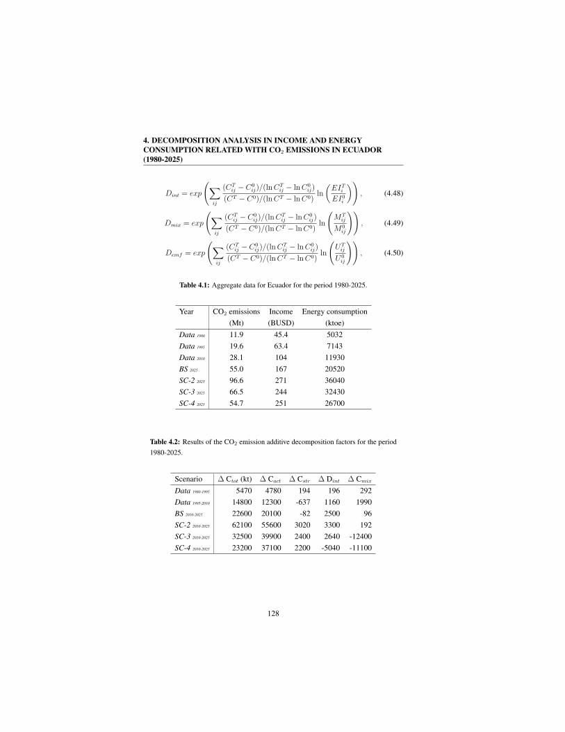
4. DECOMPOSITION ANALYSIS IN INCOME AND ENERGY
CONSUMPTION RELATED WITH CO2 EMISSIONS IN ECUADOR
(1980-2025)
Dint = exp
(
∑
ij
(CTij − C0
ij)/(lnCTij − lnC0
ij)
(CT − C0)/(lnCT − lnC0)ln
(
EITiEI0i
)
)
, (4.48)
Dmix = exp
(
∑
ij
(CTij − C0
ij)/(lnCTij − lnC0
ij)
(CT − C0)/(lnCT − lnC0)ln
(
MTij
M0ij
))
, (4.49)
Demf = exp
(
∑
ij
(CTij − C0
ij)/(lnCTij − lnC0
ij)
(CT − C0)/(lnCT − lnC0)ln
(
UTij
U0ij
))
, (4.50)
Table 4.1: Aggregate data for Ecuador for the period 1980-2025.
Year CO2 emissions Income Energy consumption
(Mt) (BUSD) (ktoe)
Data 1980 11.9 45.4 5032
Data 1995 19.6 63.4 7143
Data 2010 28.1 104 11930
BS 2025 55.0 167 20520
SC-2 2025 96.6 271 36040
SC-3 2025 66.5 244 32430
SC-4 2025 54.7 251 26700
Table 4.2: Results of the CO2 emission additive decomposition factors for the period
1980-2025.
Scenario ∆ Ctot (kt) ∆ Cact ∆ Cstr ∆ Dint ∆ Cmix
Data 1980-1995 5470 4780 194 196 292
Data 1995-2010 14800 12300 -637 1160 1990
BS 2010-2025 22600 20100 -82 2500 96
SC-2 2010-2025 62100 55600 3020 3300 192
SC-3 2010-2025 32500 39900 2400 2640 -12400
SC-4 2010-2025 23200 37100 2200 -5040 -11100
128
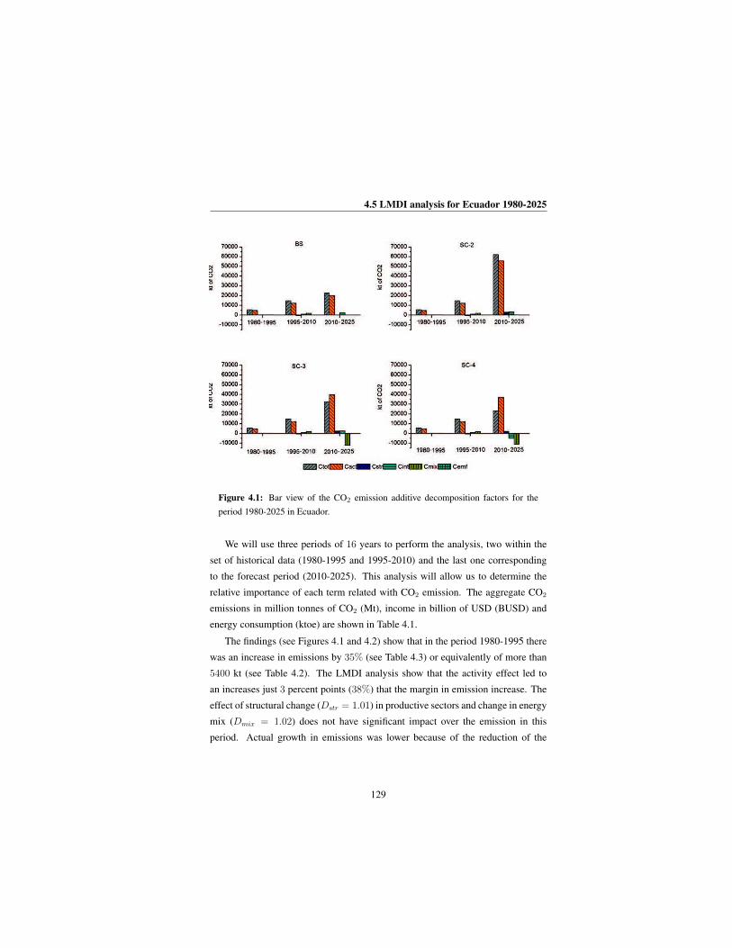
4.5 LMDI analysis for Ecuador 1980-2025
Figure 4.1: Bar view of the CO2 emission additive decomposition factors for the
period 1980-2025 in Ecuador.
We will use three periods of 16 years to perform the analysis, two within the
set of historical data (1980-1995 and 1995-2010) and the last one corresponding
to the forecast period (2010-2025). This analysis will allow us to determine the
relative importance of each term related with CO2 emission. The aggregate CO2
emissions in million tonnes of CO2 (Mt), income in billion of USD (BUSD) and
energy consumption (ktoe) are shown in Table 4.1.
The findings (see Figures 4.1 and 4.2) show that in the period 1980-1995 there
was an increase in emissions by 35% (see Table 4.3) or equivalently of more than
5400 kt (see Table 4.2). The LMDI analysis show that the activity effect led to
an increases just 3 percent points (38%) that the margin in emission increase. The
effect of structural change (Dstr = 1.01) in productive sectors and change in energy
mix (Dmix = 1.02) does not have significant impact over the emission in this
period. Actual growth in emissions was lower because of the reduction of the
129
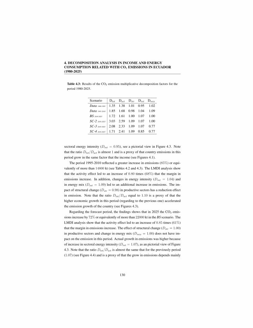
4. DECOMPOSITION ANALYSIS IN INCOME AND ENERGY
CONSUMPTION RELATED WITH CO2 EMISSIONS IN ECUADOR
(1980-2025)
Table 4.3: Results of the CO2 emission multiplicative decomposition factors for the
period 1980-2025.
Scenario Dtot Dact Dstr Dint Dmix
Data 1980-1995 1.35 1.38 1.01 0.95 1.02
Data 1995-2010 1.85 1.68 0.98 1.04 1.09
BS 2010-2025 1.72 1.61 1.00 1.07 1.00
SC-2 2010-2025 3.03 2.59 1.09 1.07 1.00
SC-3 2010-2025 2.08 2.33 1.09 1.07 0.77
SC-4 2010-2025 1.71 2.41 1.09 0.85 0.77
sectoral energy intensity (Dint = 0.95), see a pictorial view in Figure 4.3. Note
that the ratio Dtot/Dact is almost 1 and is a proxy of that country emissions in this
period grow in the same factor that the income (see Figures 4.1).
The period 1995-2010 reflected a greater increase in emissions (85%) or equi-
valently of more than 14800 kt (see Tables 4.2 and 4.3). The LMDI analysis show
that the activity effect led to an increase of 0.80 times (68%) that the margin in
emissions increase. In addition, changes in energy intensity (Dint = 1.04) and
in energy mix (Dint = 1.09) led to an additional increase in emissions. The im-
pact of structural change (Dstr = 0.98) in productive sectors has a reduction effect
in emission. Note that the ratio Dtot/Dact equal to 1.10 is a proxy of that the
higher economic growth in this period (regarding to the previous one) accelerated
the emission growth of the country (see Figures 4.3).
Regarding the forecast period, the findings shows that in 2025 the CO2 emis-
sions increase by 72% or equivalently of more than 22000 kt in the BS scenario. The
LMDI analysis show that the activity effect led to an increase of 0.85 times (61%)
that the margin in emissions increase. The effect of structural change (Dstr = 1.00)
in productive sectors and change in energy mix (Dmix = 1.00) does not have im-
pact on the emission in this period. Actual growth in emissions was higher because
of increase in sectoral energy intensity (Dint = 1.07), as an pictorial view of Figure
4.3. Note that the ratio Dtot/Dact is almost the same that for the previously period
(1.07) (see Figure 4.4) and is a proxy of that the grow in emissions depends mainly
130
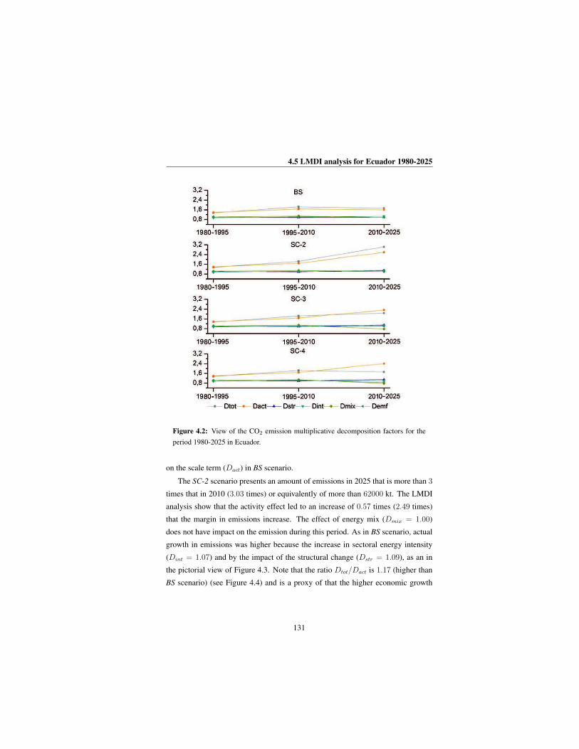
4.5 LMDI analysis for Ecuador 1980-2025
Figure 4.2: View of the CO2 emission multiplicative decomposition factors for the
period 1980-2025 in Ecuador.
on the scale term (Dact) in BS scenario.
The SC-2 scenario presents an amount of emissions in 2025 that is more than 3
times that in 2010 (3.03 times) or equivalently of more than 62000 kt. The LMDI
analysis show that the activity effect led to an increase of 0.57 times (2.49 times)
that the margin in emissions increase. The effect of energy mix (Dmix = 1.00)
does not have impact on the emission during this period. As in BS scenario, actual
growth in emissions was higher because the increase in sectoral energy intensity
(Dint = 1.07) and by the impact of the structural change (Dstr = 1.09), as an in
the pictorial view of Figure 4.3. Note that the ratio Dtot/Dact is 1.17 (higher than
BS scenario) (see Figure 4.4) and is a proxy of that the higher economic growth
131

4. DECOMPOSITION ANALYSIS IN INCOME AND ENERGY
CONSUMPTION RELATED WITH CO2 EMISSIONS IN ECUADOR
(1980-2025)
Figure 4.3: Pictorial view of the CO2 emission multiplicative decomposition factors
for the period 1980-2025 in Ecuador.
achieved in this scenario is because an increase in the economic scale and in the en-
ergy intensity, arising from the shift in the composition of industry output towards
energy-intensive sectors of the country as has been considered in this scenario (see
Section 3.10.2 in Chapter 3).
The SC-3 scenario presents an amount of emissions in 2025 that is more than
2 times in 2010 (2.08 times) or equivalently of more than 32000 kt. The LMDI
analysis show that the activity effect led to an increase of 1.23 times (Dtot = 2.33)
that the margin in emissions increase. In addition, impact of structural change
(Dstr = 1.09) in productive sectors changes and in energy intensity (Dint = 1.07)
led to a increase in emissions. The impact of energy mix (Dstr = 0.77) used in
productive sectors has a reduction effect in emissions as has been considered in
this scenario (see Section 3.10.2 in Chapter 3), see a pictorial view in Figure 4.3.
Note that the ratio Dtot/Dact is lower than 1 (0.89) (see Figure 4.4) and is a proxy
of that for first time in the country (in the analyzed period), the economic growth
is higher than emission growth. The reason is that in addition of the growth in the
economic scale, the impact of energy mix change leads to a reduction of this ratio.
Finally, in the SC-4 scenario the emissions just increase by a factor of 1.71
or equivalently more than 23000 kt. The LMDI analysis shows that the activity
132
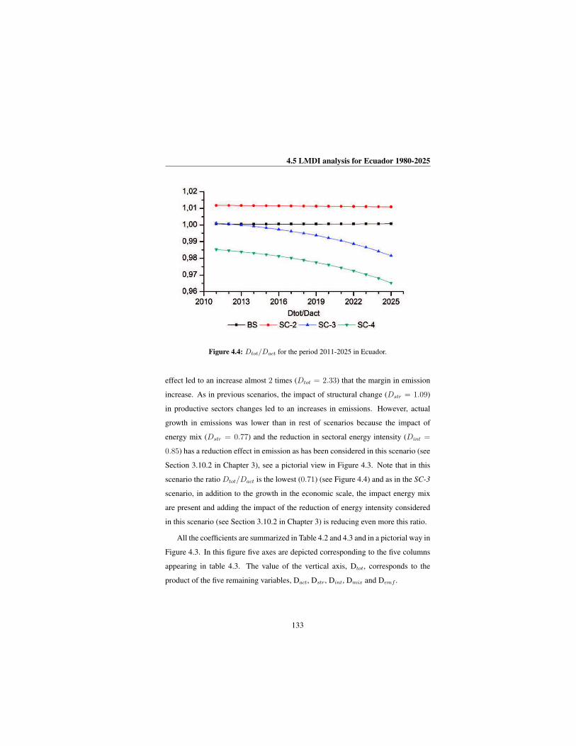
4.5 LMDI analysis for Ecuador 1980-2025
Figure 4.4: Dtot/Dact for the period 2011-2025 in Ecuador.
effect led to an increase almost 2 times (Dtot = 2.33) that the margin in emission
increase. As in previous scenarios, the impact of structural change (Dstr = 1.09)
in productive sectors changes led to an increases in emissions. However, actual
growth in emissions was lower than in rest of scenarios because the impact of
energy mix (Dstr = 0.77) and the reduction in sectoral energy intensity (Dint =
0.85) has a reduction effect in emission as has been considered in this scenario (see
Section 3.10.2 in Chapter 3), see a pictorial view in Figure 4.3. Note that in this
scenario the ratio Dtot/Dact is the lowest (0.71) (see Figure 4.4) and as in the SC-3
scenario, in addition to the growth in the economic scale, the impact energy mix
are present and adding the impact of the reduction of energy intensity considered
in this scenario (see Section 3.10.2 in Chapter 3) is reducing even more this ratio.
All the coefficients are summarized in Table 4.2 and 4.3 and in a pictorial way in
Figure 4.3. In this figure five axes are depicted corresponding to the five columns
appearing in table 4.3. The value of the vertical axis, Dtot, corresponds to the
product of the five remaining variables, Dact, Dstr, Dint, Dmix and Demf .
133
4. DECOMPOSITION ANALYSIS IN INCOME AND ENERGY
CONSUMPTION RELATED WITH CO2 EMISSIONS IN ECUADOR
(1980-2025)
4.6 Summary and conclusions of the chapter
This Chapter presents a decomposition analysis of CO2 related to income growth
and energy consumption bases on LMDI (see Section 4.5 in this Chapter) for
Ecuador in the period 1980-2025. For this purpose three periods have been se-
lected, the first sub-period is 1980-1995 where the LMDI analysis findings suggest
that the country emissions in this period almost grow (38%) in the same factor that
the income (35%), see Figures 4.1. The second sub-period is 1995-2010 and the
evidence suggest that a higher economic growth (68%) led to even greater emis-
sions growth (85%) in the country.
The third sub-period is 2010-2025 and includes the analysis for the different
scenarios proposed in Chapter 3. To see more clearly how the income-CO2 rela-
tionship behaves as a function of time, it is very enlightening to depict the ratio
Dtot/Dact as a function of the time (see Figure 4.4). The first striking thing is the
very different behaviour for each scenario. On one hand, it is somehow surprising
the almost flat curve corresponding to the BS scenario which implies a trend-growth
GDP scenario, however the CO2 emission increases steadily because of the absence
of attenuation measurements. A similar behaviour, although slightly sloping down,
is observed for SC-2, where a rapid growth of the GDP is assumed without any
attenuation action regarding CO2 emission. It is worth noting a certain decrease
of the ratio Dtot/Dact in the final part of the period under study. The other two
scenarios, SC-3 and SC-4, show a steady reduction of the ratio Dtot/Dact due to the
changes in the sectoral structure and in the energy mix, which allows compensation
of rapid GDP growth.
This preliminary analysis suggests that, with the appropriate changes in the
energy mix, the sectoral structure, and the share of renewable energies, Ecuador
can move into a more environmentally sustainable situation. All these results en-
courages us to perform a more rigorous analysis in regard to income and emission
relationship. The EKC analysis to study in which stage of the process Ecuador is
currently in, and will be in the coming future is carried out in Chapter 5.
134
You must be the change you wish to
see in the world.
Mahatma Gandhi
CHAPTER
5System dynamics modelling
and the environmental
Kuznets curve in Ecuador
(1980-2025)
5.1 Overview
Kuznets (1955) stated that the changing relationship between per capita income and
income inequality is an inverted-U-shaped curve. As per capita income increases,
income inequality also increases at first and then starts declining after a turning
point (TP). In other words, the distribution of income becomes more unequal in
early stage of income growth and then the distribution moves towards greater equal-
ity as economic growth continues (Kuznets, 1955) [88]. This observed empirical
phenomenon is popularly known as the Kuznets curve. In the 1990s and onwards,
the Kuznets curve took a new existence. There were evidences that the level of
environmental degradation and the per capita income follows the same inverted-U-
shaped relationship as does income inequality and per capita income in the original
135
5. SYSTEM DYNAMICS MODELLING AND THE ENVIRONMENTAL
KUZNETS CURVE IN ECUADOR (1980-2025)
Kuznets curve. Now, Kuznets curve has become a tool for describing the relation-
ship between measured levels of environmental quality (for example, emissions of
CO2) and per capita income. This inverted-U-shaped relationship between eco-
nomic growth and measured pollution indicators (environmental quality) is known
as the Environmental Kuznets curve (EKC).
First empirical EKC studies appeared independently in three working papers:
an NBER1 working paper as part of a study of the environmental impacts of NAFTA2
(Grossman and Krueger, 1991) [131], the World Bank’s 1992 World Development
Report (Shafik and Bandyopadhyay, 1992) [92] and a Development Discussion pa-
per as part of a study for the International Labour Organisation (Panayotou, 1993)
[223]. Grossman and Krueger which was later published in 1993 (Grossman and
Krueger, 1993) [131], first pointed out an inverted-U relationship between pollut-
ants (SO2 and smoke) and income per capita. The name of Kuznets was attached to
the inverted-U relationship between pollution and economic development later due
to its resemblance with the inverted-U relationship between income inequality and
economic development proposed by Kuznets. However, Panayotou (1993) [223]
first coined it as the Environmental Kuznets curve or EKC. At this point we will
follow the review that Dinda (2004) [93] conducted about the EKC hypothesis.
5.2 Explanations for the EKC
EKC hypothesis actually summarizes an essentially dynamic process of change. As
income of an economy grows over time, emission level grows first, reaches a peak
and then starts declining after a threshold level of income has been crossed. How-
ever, the statement of the hypothesis makes no explicit reference to time. Dinda
(2004) [93] states that EKC can be considerate as a long run phenomenon. In other
words, it is a development trajectory for a single economy that grows through dif-
ferent stages over time. Empirically, this development trajectory can be observed
in cross-country or cross-sectional data, which represents countries with different
1The National Bureau of Economic Research is an American private nonprofit research or-
ganization committed to undertaking and disseminating unbiased economic research among public
policymakers, business professionals, and the academic community.2North American Free Trade Agreement.
136

5.2 Explanations for the EKC
Figure 5.1: Different effects of income on environmental degradation as presented in
Islam et al. (1999) [7]
level of income (low, middle and high) groups corresponding to their emission
levels. The author also said that assuming that all countries follow one EKC, then
at any cross-section of time, it should be observed that some countries are poor,
shaping the initial stage of EKC, some others are developing countries approach-
ing towards the peak or starting to decline and others are rich, lying on the final
stage of the EKC. Evidently, thus, under the null hypothesis of EKC and under
the assumption of invariance of the income–emission relationship, for a given set
of cross-country or cross-sectional data on income and emission, the emission on
income regression line should be an inverted-U-shaped empirical EKC [93].
Therefore, according to the EKC hypothesis the relationship between income
per capita and some types of pollution is approximately an inverted-U. This beha-
viour states that as the per capita income growths, environmental damage increases,
reaches a maximum, and then declines. The reason for this behaviour is that when
income reaches a certain threshold the economy moves into a different regime,
where the rate of emissions with respect to income can be reduced with respect to
the initial regime.
There is thus a unidirectional causality running from income to environmental
degradation. The theoretical explanations of the EKC hypothesis are based on three
effects: the scale effect, the structure effect and the abatement effect (Grossman and
Krueger,1991; Islam etal.,1999) [7, 131] (see Figure 5.1).
137
5. SYSTEM DYNAMICS MODELLING AND THE ENVIRONMENTAL
KUZNETS CURVE IN ECUADOR (1980-2025)
5.2.1 Environmental quality demand and income elasticity
As income grows, society achieve a higher standard of living and care more for
the quality of environment they live in and demand for better environment induces
structural changes in economy that tends to reduce environmental degradation. The
most common explanation for the shape of an EKC (see Figure 5.2) is the notion
that when a country achieves a sufficiently high standard of living, people attach
increasing value to environmental amenities (Pezzey, 1989 [224]; Selden and Song,
1994 [225]; Baldwin, 1995 [226]). When a particular level of income is reached,
the willingness to pay for a clean environment rises by a greater proportion than
income (Roca, 2003) [227]. This will be reflected through changes in habits and
in choice of less environmentally damaging products by people. Thus, people with
a high standard of living can value and pay (at the same time) for a cleaner en-
vironment and to preserve it. Generally, it is recognized that income elasticity of
environmental quality demand and resource goods is in excess of unity, i.e., clean
environment and preservation are luxury goods [93]. But major indicators of en-
vironmental degradation are monotonically rising in income though the income
elasticity is less than one and is not a simple function of income alone [93]. How-
ever, Dinda (2004) survey [93] states that most of the EKC models have emphas-
ized the role of income elasticity of environmental quality demand (Beckerman,
1992 [91]; Carson et al., 1997 [228]; Chaudhuri and Pfaff, 1998 [229]; McCon-
nell, 1997 [230]) and this elasticity is often invoked in the literature as the main
reason to explain the reduction of emission level. An adequate explanation of ob-
served EKC relationships for some pollutants, are consistent with the high-income
elasticity of environmental quality demand (McConnell, 1997 [230]; Shafik, 1994
[231]). Poor countries have little demand for environmental quality, however, as
a society reaches high levels of living , its members may intensify their demands
for a more healthy and cleaner environment. Societies with higher incomes are not
only willing to spend more for green products but also create pressure for envir-
onmental protection and regulations. In most cases where emissions have declined
with rising income, the reductions have been due to local and national institutional
reforms, such as environmental legislation and market-based incentives to reduce
environmental degradation.
138

5.2 Explanations for the EKC
5.2.2 Scale, technological and composition effects
There are three different channels where economic growth affects the quality of en-
vironment: scale effects, technological effects and composition effects (Grossman
and Krueger, 1991) [131]. Increasing output requires more input and thus more
natural resources are used in production process. More output also implies more
wastes and emissions by product, which also contributes to degrade environmental
quality. Therefore, economic growth exhibits a scale effect that has a negative im-
pact on environment. However, economic growth also has a positive impact on
environment through the composition effect: income grows, the structure of the
economy tends to change and gradually cleaner activities increase with reduces
pollution [93].
Environmental degradation tends to increase as structure of the economy changes
from rural to urban, or from agricultural to industrial, but it starts to fall with an-
other structural change from energy intensive industry to services and knowledge
based technology intensive industry. As a wealthy nation can afford to spend more
on research and technical development (Komen et al., 1997) [135], technological
progress occurs with economic growth and the dirty and obsolete technologies are
replaced by upgraded new and cleaner technology, which improves environmental
quality. This is the so called technique effect of economic growth. Vukina et al.,
(1999) [132] state that EKC suggests that the negative impact on environment of
the scale effect, that tends to prevail in initial stages of growth, will be eventually
outweighed by the positive impact of the composition and technique effects that
will tend to lower the emission level.
5.2.3 International trade
International trade is one of the most important factors that envelope the EKC [93].
Trade leads to increase the size of the economy increasing pollution, thus, trade can
be considerate as a cause of environmental degradation. However, many authors
have long argued that trade is not the root cause of environmental damage (Birdsall
and Wheeler, 1993 [232]; Lee and Roland-Holst, 1997 [233]; Jones and Rodolfo,
1995 [234]). Free trade has the contradictory impacts on environment, on one hand,
139

5. SYSTEM DYNAMICS MODELLING AND THE ENVIRONMENTAL
KUZNETS CURVE IN ECUADOR (1980-2025)
increasing pollution and, on the other hand, motivating reductions in it. Environ-
mental quality could decline through the scale effect as increase the trade volume
(especially export) up to the size of the economy, which increases pollution. On
the other hand, trade can improve the environment through the composition ef-
fect and/or the technique effect (i.e., as income rises through trade, environmental
regulation is tightened whith spurs pollution reducing innovation) [93].
Pollution from the production of pollution-intensive goods declines in a given
country as it increases in an other via international trade. This composition effect
is attributed to two related hypotheses: i) Displacement Hypothesis and ii) Pol-
lution Haven Hypothesis. These hypotheses are basically the same with respect
to comparative advantage in international trade. Displacement Hypothesis expects
that trade liberalization or openness will lead more rapid growth of pollution- in-
tensive industries in less developed economies as developed economies enforce
strict environmental regulations (Harrison, 1996 [235]; Rock, 1996 [236]; Tobey,
1990 [237])1. Pollution Haven Hypothesis refers to the possibility that multina-
tional industries, particularly those engaged in highly polluting activities, relocate
to countries with lower environmental standards. Also this hypothesis argues that
low environmental standards become a source of comparative advantage, and thus
shifts in trade patterns. This theory suggests that high regulation countries will lose
all the dirty industries and low regulation countries will get them all.
Most of the developing countries rely on technology transfer through foreign
direct investment from developed countries as a primary means of technology ac-
quisition. In the case of Pollution Haven Hypothesis, these clean and upgraded
technologies could reduce pollution level. Also the diffusion of technology pre-
vents economic latecomers from requiring the same levels of materials and en-
ergy inputs per unit of income than older industrialized countries needed in past.
Some authors suggest that international trade enhances diffusion of clean techno-
logy (Martin and Wheeler, 1992 [238]; Reppelin-Hill, 1999 [239]) and another
authors have suggested that this might allow developing countries to dive through
the EKC.
1Note that, the changes in the structure of production in developed economies are not accom-
panied by equivalent changes in the structure of consumption, therefore, EKC actually records
displacement of dirty industries to less developed economies (Copeland and Taylor, 1995) [123].
140

5.3 Theoretical analysis of EKC
Other scenario could be the so called race to bottom: relatively high environ-
mental standards in developed economies impose high costs on polluters. There-
fore, polluting activities in high-income economies face higher regulatory costs
than their counterparts in developing countries (Wheeler, 2000 [240] and Jaffe et
al., 1995 [241]; Mani, 1998 [242]). Wheeler (2000) [240] states that globalization
could trigger the environmental race to bottom, in which competition increases
for investment and jobs. Indeed, the bottom rises with economic growth. Less
developed economies improve their environmental quality as investment increases
income and employment. This has led some authors to argue that globalization is
compatible with pollution reduction (Robinson, 1988 [243]; Dessus and Bussolo,
1998 [244]; Grether and Melo, 2002 [245]).
5.3 Theoretical analysis of EKC
A basic comparative static analysis of the costs and benefits associated with a better
environmental quality provides an interesting conceptual insight as to how the EKC
may arise. The EKC is derived from the interaction points of marginal cost (MC)
and marginal benefit (MB) curves (Munasinghe, 1999) [140]. An EKC can be
derived directly from the technological link between consumption of a desired good
and abatement of its undesirable by product (Andreoni and Levinson, 2001) [246].
It is also consistent with either Pareto1 efficient policy or a decentralized market
economy. If pollution is not priced, companies will use it until its marginal product
is zero, when pollution is considered as a factor of production, but not the stock
of environmental capital. Extending this model, stock of environmental quality is
included as a factor of production (Lopez, 1994) [247], then the predictions of this
model depend crucially on the existence of property rights. The EKC emerges from
a dynamic process, as a part of capital goes for development of the environmental
sectors. Total capital is divided into two parts, one is used in production process
that creates pollution and damage the existing environment and the other is used to
clean up environment or improve it (Dinda, 2002) [114].
1Pareto efficiency, or Pareto optimality, is a state of allocation of resources in which it is im-
possible to make any one individual better off without making at least one individual worse off.
141
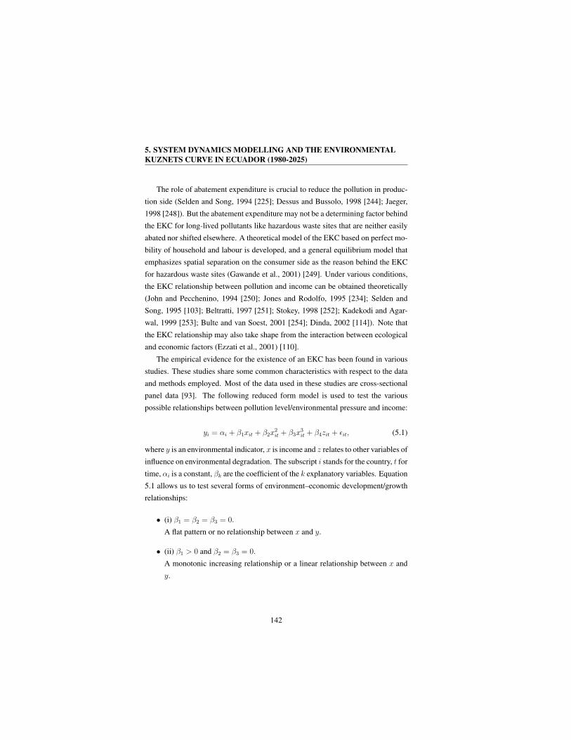
5. SYSTEM DYNAMICS MODELLING AND THE ENVIRONMENTAL
KUZNETS CURVE IN ECUADOR (1980-2025)
The role of abatement expenditure is crucial to reduce the pollution in produc-
tion side (Selden and Song, 1994 [225]; Dessus and Bussolo, 1998 [244]; Jaeger,
1998 [248]). But the abatement expenditure may not be a determining factor behind
the EKC for long-lived pollutants like hazardous waste sites that are neither easily
abated nor shifted elsewhere. A theoretical model of the EKC based on perfect mo-
bility of household and labour is developed, and a general equilibrium model that
emphasizes spatial separation on the consumer side as the reason behind the EKC
for hazardous waste sites (Gawande et al., 2001) [249]. Under various conditions,
the EKC relationship between pollution and income can be obtained theoretically
(John and Pecchenino, 1994 [250]; Jones and Rodolfo, 1995 [234]; Selden and
Song, 1995 [103]; Beltratti, 1997 [251]; Stokey, 1998 [252]; Kadekodi and Agar-
wal, 1999 [253]; Bulte and van Soest, 2001 [254]; Dinda, 2002 [114]). Note that
the EKC relationship may also take shape from the interaction between ecological
and economic factors (Ezzati et al., 2001) [110].
The empirical evidence for the existence of an EKC has been found in various
studies. These studies share some common characteristics with respect to the data
and methods employed. Most of the data used in these studies are cross-sectional
panel data [93]. The following reduced form model is used to test the various
possible relationships between pollution level/environmental pressure and income:
yi = αi + β1xit + β2x2it + β3x
3it + β4zit + ǫit, (5.1)
where y is an environmental indicator, x is income and z relates to other variables of
influence on environmental degradation. The subscript i stands for the country, t for
time, αi is a constant, βk are the coefficient of the k explanatory variables. Equation
5.1 allows us to test several forms of environment–economic development/growth
relationships:
• (i) β1 = β2 = β3 = 0.
A flat pattern or no relationship between x and y.
• (ii) β1 > 0 and β2 = β3 = 0.
A monotonic increasing relationship or a linear relationship between x and
y.
142

5.4 Empirical findings of EKC in Ecuador
• (iii) β1 < 0 and β2 = β3 = 0.
A monotonic decreasing relationship between x and y.
• (iv) β1 > 0, β2 < 0 and β3 = 0.
An inverted-U-shaped relationship, i.e., EKC.
• (v) β1 < 0, β2 > 0 and β3 = 0.
A U-shaped relationship.
• (vi) β1 > 0, β2 < 0 and β3 > 0.
A cubic polynomial or N-shaped figure.
• (vii) β1 < 0, β2 > 0 and β3 < 0.
Opposite to the N-shaped curve.
5.4 Empirical findings of EKC in Ecuador
The inverted U-shaped relationship between CO2 emissions and GDP is an empir-
ical observation. In this respect there are many studies where quadratic and cubic
models are used to fit the emissions to income (Canas, 2003 [255]; Shen, 2004
[256]; Cole, 2005 [257]; Galeotti, 2006 [258]; Esteve, 2012a [259]). However, in
many cases the evidences of the EKC hypothesis is weak. Another way to test the
validity of the EKC assumption is to compare the long and the short run impact
of income on emissions (Nara, 2010 [260], Jaunky, 2011 [145]). Whatever ap-
proach is used or set of countries studied, analysis always uses past data and there
are no studies where the EKC hypothesis has been tested in a forthcoming period.
To do this, a detailed model of the connection between GDP and CO2 emissions
is needed, as well as a set of plausible scenarios that could describe a possible
evolution (income, energy matrix, and sectoral structure) of a given country.
As the theory predicts a long-run relationship linking emissions and economic
growth, there is a wide stream of recent research that has assessed this relation-
ship employing co-integration techniques. The empirical evidence suggests that
pollution levels and GDP may be jointly determined, so that any constraint put
on energy consumption, to help in reducing emissions, will have effects on eco-
nomic growth. In the initial stage, as in the developing countries, CO2 emissions
143
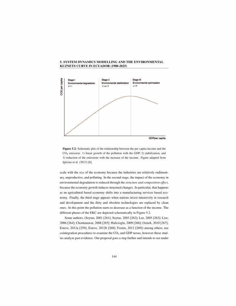
5. SYSTEM DYNAMICS MODELLING AND THE ENVIRONMENTAL
KUZNETS CURVE IN ECUADOR (1980-2025)
Figure 5.2: Schematic plot of the relationship between the per capita income and the
CO2 emission: 1) linear growth of the pollution with the GDP, 2) stabilization, and
3) reduction of the emissions with the increase of the income. Figure adapted from
Iglesias et al. (2013) [8].
scale with the size of the economy because the industries are relatively rudiment-
ary, unproductive, and polluting. In the second stage, the impact of the economy in
environmental degradation is reduced through the structure and composition effect,
because the economy growth induces structural changes. In particular, that happens
as an agricultural based economy shifts into a manufacturing services based eco-
nomy. Finally, the third stage appears when nations invest intensively in research
and development and the dirty and obsolete technologies are replaced by clean
ones. At this point the pollution starts to decrease as a function of the income. The
different phases of the EKC are depicted schematically in Figure 5.2.
Some authors, (Soytas, 2001 [261]; Soytas, 2003 [262]; Lee, 2005 [263]; Lise,
2006 [264]; Chontanawat, 2008 [265]; Halicioglu, 2009 [266]; Ozturk, 2010 [267];
Esteve, 2012a [259]; Esteve, 2012b [268]; Fosten, 2012 [269]) among others, use
cointegration procedures to examine the CO2 and GDP nexus, however these stud-
ies analyze past evidence. Our proposal goes a step further and intends to see under
144

5.4 Empirical findings of EKC in Ecuador
what conditions a country could approach the fulfilment of the EKC hypothesis in
the medium term.
To this end, we will use the model proposed in Chapter 3 and the findings of
Chapter 4 ((see Section 4.6 in Chapter 4) as starting point (see Section 3.10.1 in
Chapter 3).
The following sections are an effort to fill the gap in the literature of studies
on the relationship between emissions and GDP in Latin American countries in
general, and in Ecuador in particular. In addition, studies of a single country help
policy makers improve comprehensive policies to control environmental degrad-
ation. Moreover, it represents a step forward in the study of the EKC hypothesis
following Jaunky’s specification [145], due to the inclusion of a forthcoming (2011-
2025) and not a past period of time.
In Jaunky (2011) the author tries to test the EKC hypothesis in a set of high-
income countries for the period 1980-2005. The lower long-run income elasticity
does not provide evidence for the EKC, but it indicates that CO2 emissions are
stabilizing in developed countries. Therefore, the extension of this work to other
countries and to a forthcoming period is of interest.
5.4.1 EKC hypothesis verification
The EKC hypothesis supposes that from a given moment onward the relationship
between CO2 emission and income is no longer proportional and that, even the first
can be reduced as GDP increases. To get the first insight about the relationship
between GDP and CO2 we plot the per capita GDP and CO2 emission as a function
of the year in Figure 5.3, using the data set of the period 1980-2010 and the model
calculation for the four considered scenarios (2011-2025). To calculate the value
of the population, needed for any per capita quantity, we use the geometric-growth
rate (Equation (3.14)) to extrapolate its value into the forecast period. Regarding
GDP, one can observe two clearly distinct behaviours in the forecast period, on one
hand the BS scenario, with a moderate increase of the GDP per capita, and on the
other hand, the rest of scenarios that present a large increase of the GDP. For CO2
emissions BS and SC-4 scenarios show the same value, while SC-3 shows a slightly
145
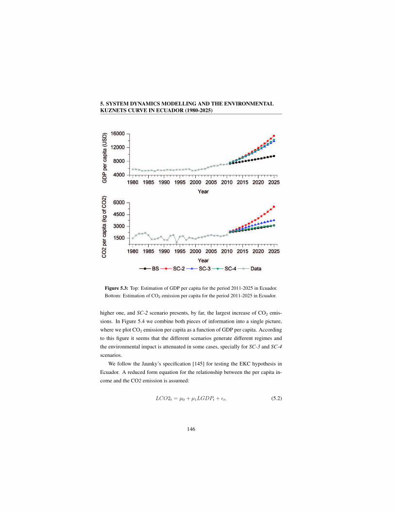
5. SYSTEM DYNAMICS MODELLING AND THE ENVIRONMENTAL
KUZNETS CURVE IN ECUADOR (1980-2025)
Figure 5.3: Top: Estimation of GDP per capita for the period 2011-2025 in Ecuador.
Bottom: Estimation of CO2 emission per capita for the period 2011-2025 in Ecuador.
higher one, and SC-2 scenario presents, by far, the largest increase of CO2 emis-
sions. In Figure 5.4 we combine both pieces of information into a single picture,
where we plot CO2 emission per capita as a function of GDP per capita. According
to this figure it seems that the different scenarios generate different regimes and
the environmental impact is attenuated in some cases, specially for SC-3 and SC-4
scenarios.
We follow the Jaunky’s specification [145] for testing the EKC hypothesis in
Ecuador. A reduced form equation for the relationship between the per capita in-
come and the CO2 emission is assumed:
LCO2t = µ0 + µ1LGDPt + ǫt, (5.2)
146

5.4 Empirical findings of EKC in Ecuador
Figure 5.4: GDP per capita versus CO2 emission per capita for the period 2011-2025
in Ecuador. Marks TP-ST1-ST2 stand for the year of the turning points (the scenario
passes from stage 1 to state 2) of the EKC (see Figure 5.5).
where LCO2 is the natural logarithm of the CO2, LGDP is the natural logarithm
of the GDP, ǫ is the error term, µ0 is the term constant, and µ1 estimates the CO2-
GDP elasticity.
In the first region of the simplified Kuznets curve (Figure 5.2), as the elasti-
city µ1 > 1 there is a high responsiveness of GDP to changes in CO2 emissions.
Therefore, a change in GDP generates a more than proportional increase in CO2
emission. This phase involves little environmental responsibility and also implies
that the country is in the early stage of environmental sustainability (environmental
degradation). If 0 < µ1 < 1, then an income increase leads to a less than propor-
tional increase in CO2 emissions and, as a consequence, it implies that the country
enters into the second stage of the EKC with environmental stabilization1 . Finally,
for µ1 < 0 a negative relationship occurs between GDP and CO2 emission. This
is the final stage of the EKC and mean that the country enters into a phase with
1Note that, we define turning point of change from the first to the second stage (TP-ST1-ST2(t)
as the time t where µ1 > 1 pass to 0 < µ1 < 1).
147

5. SYSTEM DYNAMICS MODELLING AND THE ENVIRONMENTAL
KUZNETS CURVE IN ECUADOR (1980-2025)
intensive use of green technology and environmental optimization.
5.4.2 EKC verification
We start the analysis by testing the order of integration of both variables LGDPt
and LCO2t using the tests of Ng and Perron (2001) [270]. These authors proposed
using test statistics which are a efficient modified versions of Phillip-Perron (PP)
and Augmented Dickey-Fuller (ADF) tests. Such modifications that improve the
tests do not exhibit the severe size distortions of the PP tests for errors with large
negative MA (moving average) or AR (auto-regression) roots, and they can have
substantially higher power than the PP tests.
Using the GLS detrended data ydT , the efficient modified PP tests are defined as:
MZGLSα =
(
T−1ydT − λ2)
(
2T−2
T∑
t=1
ydt−1
)−1
, (5.3)
MSBGLS =
(
T−2
T∑
t=1
ydt−1
λ2
)1/2
, (5.4)
MZGLSt = MZGLS
α × MSBGLS, (5.5)
MSBGLS =
[
T−2
(
yt−12
s2
)]1/2
, (5.6)
where [yt]T1 represents the realization of the time series, T denotes the sample size,
λ2 is a consistent estimate of the long-run variance parameter λ2 and s2 are the
variances.
The statistics MZGLSα and MZGLS
t are efficient versions of the PP and Zα and
Zt tests that have much smaller size distortions in the presence of negative moving
average errors. Note that those tests should be performed for the whole dataset.
The results are shown in Table 5.1, and according to them, the null hypothesis
of no stationarity cannot be rejected, independently of the statistic used, for both
series, LGDPt and LCO2t. Accordingly, both series would be concluded to be
I(1).
148
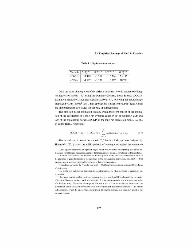
5.4 Empirical findings of EKC in Ecuador
Table 5.1: Ng-Perron unit root test.
Variable MZGLSα MZGLS
t MSBGLS MPGLST
LGDPt -3.488 -1.268 0.364 25.197
LCO2t -4.827 -1.532 0.317 18.750
Once the order of integration of the series is analyzed, we will estimate the long-
run regression model [145] using the Dynamic Ordinary Least Squares (DOLS)1
estimation method of Stock and Watson (2010) [144], following the methodology
proposed by Shin (1994)2 [271]. This approach is similar to the KPSS3 tests, which
are implemented in two stages for the case of cointegration.
The first step in our estimation strategy would therefore consist of the estima-
tion of the coefficients of a long-run dynamic equation [145] including leads and
lags of the explanatory variables (GDP) in the long-run regression model, i.e., the
so-called DOLS regression:
LCO2t = µ0 + µ1LGDPt +
q∑
j=−q
µj∆LGDPt−j + ǫj. (5.7)
The second step is to use the statistic Cµ4 that is a LM-type5 test designed by
Shin (1994) [271], to test the null hypothesis of cointegration against the alternative
1Least squares estimation of equation might suffer two problems: endogeneity bias in the ex-
planatory variables and nuisance parameter dependencies due to serial correlation in the residuals.2In order to overcome the problem of the low power of the classical cointegration tests in
the presence of persistent roots in the residuals of the cointegration regression, Shin (1994) [271]
suggests a new test where the null hypothesis is that of cointegration.3These tests are called the Kwiatkowski et al. (1992) [272] tests, and assume the null hypothesis
of stationarity.4Cµ is the test statistic for deterministic cointegration, i.e., when no trend is present in the
regression.5 Lagrange multiplier (LM) test is a statistical test of a simple null hypothesis that a parameter
of interest θ is equal to some particular value θ0. It is the most powerful test when the true value
of θ is close to θ0. The main advantage of this test is that it does not require an estimate of the
information under the alternative hypothesis or unconstrained maximum likelihood. This makes
testing feasible when the unconstrained maximum likelihood estimate is a boundary point in the
parameter space.
149
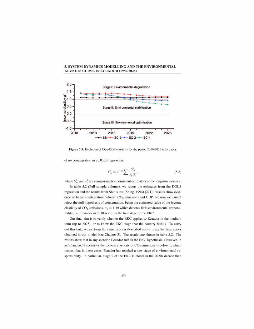
5. SYSTEM DYNAMICS MODELLING AND THE ENVIRONMENTAL
KUZNETS CURVE IN ECUADOR (1980-2025)
Figure 5.5: Evolution of CO2-GDP elasticity for the period 2010-2025 in Ecuador.
of no cointegration in a DOLS regression.
Cµ = T−2∑ S2
µt
s2µ(l), (5.8)
where S2µt and s2µ are semiparametric consistent estimators of the long-run variance.
In table 5.2 (Full sample column), we report the estimates from the DOLS
regression and the results from Shin’s test (Shing, 1994) [271]. Results show evid-
ence of linear cointegration between CO2 emissions and GDP, because we cannot
reject the null hypothesis of cointegration, being the estimated value of the income
elasticity of CO2 emissions, µ1 = 1.19 which denotes little environmental respons-
ibility, i.e., Ecuador in 2010 is still in the first stage of the EKC.
Our final aim is to verify whether the EKC applies to Ecuador in the medium
term (up to 2025), or to know the EKC stage that the country fulfills. To carry
out this task, we perform the same process described above using the time series
obtained in our model (see Chapter 3). The results are shown in table 5.2. The
results show that in any scenario Ecuador fulfills the EKC hypothesis. However, in
SC-3 and SC-4 scenarios the income elasticity of CO2 emissions is below 1, which
means, that in these cases, Ecuador has reached a new stage of environmental re-
sponsibility. In particular, stage 2 of the EKC is closer in the 2020s decade than
150
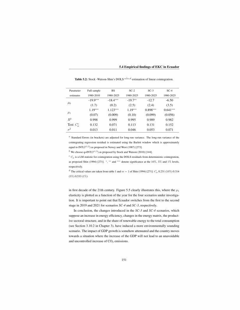
5.4 Empirical findings of EKC in Ecuador
Table 5.2: Stock -Watson-Shin’s DOLS a,b,c,d estimation of linear cointegration.
Parameter
estimates
Full sample
1980-2010
BS
1980-2025
SC-2
1980-2025
SC-3
1980-2025
SC-4
1980-2025
µ0
-19.9∗∗∗
(1.7)
-18.4∗∗∗
(0.2)
-19.7∗∗
(2.5)
-12.7
(2.4)
-6.50
(3.5)
µ1
1.19∗∗∗
(0.07)
1.123∗∗∗
(0.009)
1.19∗∗∗
(0.10)
0.898∗∗∗
(0.099)
0.641∗∗∗
(0.056)
R2 0.998 0.999 0.995 0.989 0.982
Test: Ccµ 0.132 0.071 0.113 0.131 0.152
σ2 0.013 0.011 0.046 0.053 0.071
a Standard Errors (in brackets) are adjusted for long-run variance. The long-run variance of the
cointegrating regression residual is estimated using the Barlett window which is approximately
equal to INT(T 1/2) as proposed in Newey and West (1987) [273].
b We choose q=INT(T 1/3) as proposed by Stock and Watson (2010) [144].
c Cµ is a LM statistic for cointegration using the DOLS residuals from deterministic cointegration,
as proposed Shin (1994) [271]. ∗, ∗∗ and ∗∗∗ denote significance at the 10%, 5% and 1% levels,
respectively.
d The critical values are taken from table 1 and m = 1 of Shin (1994) [271]: Cµ 0.231 (10%) 0.314
(5%) 0.533 (1%)
in first decade of the 21th century. Figure 5.5 clearly illustrates this, where the µ1
elasticity is plotted as a function of the year for the four scenarios under investiga-
tion. It is important to point out that Ecuador switches from the first to the second
stage in 2019 and 2021 for scenarios SC-4 and SC-3, respectively.
In conclusion, the changes introduced in the SC-3 and SC-4 scenarios, which
suppose an increase in energy efficiency, changes in the energy matrix, the product-
ive sectoral structure, and in the share of renewable energy to the total consumption
(see Section 3.10.2 in Chapter 3), have induced a more environmentally sounding
scenario. The impact of GDP growth is somehow attenuated and the country moves
towards a situation where the increase of the GDP will not lead to an unavoidable
and uncontrolled increase of CO2 emissions.
151
5. SYSTEM DYNAMICS MODELLING AND THE ENVIRONMENTAL
KUZNETS CURVE IN ECUADOR (1980-2025)
5.5 Summary and conclusions of the chapter
In this Chapter we have studied the EKC hypothesis for Ecuador in a forthcoming
period, 2011-2025, using the model propoused in Chapter 3 under four different
scenarios (see Section 3.10.1 in Chapter 3). The model allows us to estimate the
CO2 emission as a function of global productive activity, the energy mix and in-
dustry sectoral structure, using the system dynamics (SD) methodology. In addition
we use a GDP formation presented in Chien and Hu (2008) [5] that depends on the
renewable energy which creates a feedback mechanism that makes the model more
reliable and allows us to obtain non-trivial conclusions in the analysis. The gen-
erated data under four different scenarios closely followed Jaunky’s specification
[145] and allowed us to see whether the EKC is fulfilled, or not, in Ecuador and to
calculate the elasticity between GDP and CO2 emission.
In the analysis of the EKC hypothesis we conclude that in any case Ecuador ful-
fills this hypothesis, but the value of the CO2-GDP elasticity allows us to separate
the proposed scenarios in two families, on one hand BS and SC-2, and, on the other,
SC-3 and SC-4 scenarios. In the first case, the elasticity is larger than one, while
in the second case it is lower than one. Therefore, the first family implies little
environmental respect, while the second family corresponds to a situation where
the impact of the GDP growth is attenuated.
Our estimates do indeed show that Ecuador will be able to enter the area of en-
vironmental stability (second stage of the EKC) in the medium term (2019-2021).
Therefore, to achieve this goal it is essential to implement policies that allow the
diversification of energy sources and to increase energy efficiency in the productive
sectors in order to get more sustainable development.
This Chapter intended to fill the gap in the literature of studies on energy and
CO2 emissions in Latin American countries in general, and in Ecuador in particular.
On the other hand, this kind of study may help policymakers create more compre-
hensive and reliable policies for control of environmental degradation. Moreover
this work contributes to the EKC literature with a case study of Ecuador using time
series data for the period 1980-2010 and goes a step further with the study of a
forthcoming period, up to 2025.
152
Our species needs, and deserves, a
citizenry with minds wide awake
and a basic understanding of how
the world works.
Carl Sagan CHAPTER
6Summary and conclusions
Globally, CO2 is by far the main contributor to anthropogenic greenhouse gas
(GHG) emissions (IPCC, 2007) [156, Fig. 2.1]: CO2 represents 76.7% of the GHG
emissions (approximately 56.6% is from fossil fuels, 17.3% from deforestation,
and 2.8% from other sources). Ecuador has a relatively low level of CO2 emissions
(2200 kg per capita) while Qatar, the world’s largest CO2 emitter per capita in
2010, emitted 40300 kg per capita. At the same time Venezuela, the largest CO2
emitter in Latin America (LA), emitted annually 6900 kg per capita (WB, 2014)
[151]. It is expected that social and economic development in the coming years
could significantly increase Ecuador’s emissions. Observations show that global
CO2 emissions, far from stabilizing, have experienced significant growth in recent
years.
Several international organizations, notably, the Intergovernmental Panel on
Climate Change (IPCC), are warning about the need of stabilizing the CO2 and oth-
ers anthropogenic GHG emissions in order to avoid a catastrophic warming of the
climatic system during this century (IPCC, 2007) [156]. The IPCC has developed
several methods to estimate GHG emissions, such as the Reference Method (IPCC,
2006) [42], which is a top-down technique that uses data from the country’s en-
ergy supply (mainly from the burning of fossil fuels), land use, and deforestation
rate, among others, to calculate CO2 emissions. It is a straightforward method that
153
6. SUMMARY AND CONCLUSIONS
can be applied on the basis of the available energy supply statistics (IPCC, 2006)
[42]. However, the problem arises when it is necessary to conduct more detailed
studies and find the driving forces that are behind the emissions, but the data is not
available or is not sufficiently disaggregated for use with this method.
A key factor of economic development in countries and the transition from sub-
sistence agricultural economies to modern industrial societies which are oriented
to services, is to have an adequate supply of affordable energy. Energy is essential
to enhance the social and economic welfare and, in most cases, it is essential to
attract industrial and commercial wealth. It is a condition, sine qua non. of poverty
alleviation, generalize social protection and raise living standards. Note that no
matter how essential energy can be for the development, energy is just a medium,
it is not the final goal, and the final goal of sustainable development is to achieve
good health, a high standard of living, sustainable energy and a clean environment.
As already mentioned, energy consumption is one of the greatest measures of
progress and well-being of a society. The concept of energy crisis appears when
the energy sources of the society supplies are depleted. An economic model like
the present one, whose operation depends on continued growth, also requires an
equally growing demand for energy. Since fossil energy sources are finite, it is
inevitable that at some point the demand can not be supplied and all system will
collapse; unless new sources of energy would be discovered or new techniques are
developed, as would be the case of renewable energy.
The potential of renewable energy has a great capacity to help meet global
energy demand. Furthermore, this type of clean energy has a rapidly growing due
to the remarkable technical advances that have taken place in recent years and by
the strong support of the various national governments and the enormous social
support.
The commitment to promote this type of development and the rational use of
energy, involves setting goals at national and regional levels and define a policy
according with these goals.
The general objective of this research was create to a useful methodology to
estimate CO2 emissions of a given country, in particular for Ecuador, and to under-
stand the driving forces that guide this process, such as economic growth, energy
use, energy mix structure, and fuel use in the productive sectors. The proposed
154
methodology tries to be easily transferable to other countries, regions, and time
periods and to be used as a pedagogical tool for explaining to policymakers the
possible ways to design a policy for reducing CO2 emissions in a medium term
horizon.
This study combines decomposition analysis with scenario modelling to create
a baseline prevision as guidance for possible new policies. This allowed the de-
velopment of a model with a set of integrated exploratory scenarios about income
growth, energy use and CO2 emissions for Ecuador in a medium term (2025). The
scenarios show plausible more environmental-friendly pathways that the country
could take to get closer to a sustainable development.
The application of scenario analysis-modelling in the short-to-medium term is
intended to develop insights into plausible future changes with additional green
goals in the driving forces in national policies. While the decomposition analysis
gives insights into historical change. The study offers potential longer-term in-
sights through the exploration of changes in to the driving forces to evaluate the
fulfillment of the Environmental Kuznets Curve (EKC) hypothesis.
The thesis was organized into six chapters and seven appendices. Chapter 1
presents the introduction of the most important aspects of the methodology and
objectives of the research. Chapter 2 introduce the main figures in economy, pro-
ductive sectors, energy use, etc., about Ecuador from 1980 to 2010; also it discusses
about critical factors for the adoption of renewable technologies in the country.
Chapter 3 presents a model approach of CO2 emissions in Ecuador in the up-
coming years, up to 2025. The main goal here is to study in detail the way the
changes in the energy matrix and in the Gross Domestic Product (GDP) will affect
the CO2 emissions in the country. In particular, special attention to the effect of
a reduction of the share of fossil energy will be paid, as well as of an improve-
ment in the efficiency of the fossil energy use. In this chapter, we have developed
a System Dynamic (SD) model based on a relationship, which is a variation of
the Kaya identity (Kaya, 1993) [169], and on a formation of GDP approach that
depends on renewable energy (Chien and Hu) [5], which introduces a feedback
mechanism in the model and allows us to generate a non-trivial evolution of the
system. Therefore, the GDP and the energy intensity have been modeled with dif-
ferent scenarios that present the evolution of the energy matrix and the productive
155

6. SUMMARY AND CONCLUSIONS
sectoral structure have been defined. First, a BS scenario (baseline scenario) has
been defined, in which the variables of the model were parameterized according
to the observed tendency during the period 1980-2010 (see Chapter 2), assuming
a geometric growth rate during the period 2011-2025. The second scenario, called
SC-2, is characterized by the increasing (relative to 2010) of the GDP during the
period 2011-2025 (with the goal of reaching the estimated international average
GDP per capita in 2025). In the third scenario, called SC-3 scenario, besides as-
suming the increasing of the GDP, we impose the decreasing of the fossil energy
share (ES1) up to 67%. Finally, in the fourth one, SC-4 scenario, we complement
the SC-3 scenario including changes in the productive sectoral structure to achieve
a reduction of energy intensity, which supposes a lower CO2 intensity.
The main outcome of this chapter are the estimates of CO2 emissions for the
period 2011-2025 in each scenario (see Section 3.11.3 in this Chapter). By 2025 the
BS scenario reaches 55 thousand kt, in the SC-2 scenario it corresponds to 97 thou-
sand kt, in SC-3 scenario to 66 thousand kt, and in the SC-4 scenario to 55 thousand
kt of CO2. Note that the BS scenario corresponds to a modest GDP increase, while
in the others the GDP increases heavily. The highest emissions are for the SC-2
scenario where no mitigation measures are taken. The other two scenarios show us
that it is possible a sizable reduction of the emissions, promoting the renewable en-
ergy (SC-3 scenario) and on top of that modifying the productive sectoral structure,
therefore, reducing the energy and the CO2 intensities, as in the SC-4 scenario. It
is worth to note that both promotion of renewable energy and improvement of the
energy intensity are equally effective attenuating CO2 emissions.
After the study that has been carried out in this chapter, the main conclusions
are:
• Energy and emissions analysis, the development of policy and the reporting
of progress require insight into the driving forces of change and potential
future evolution.
• Energy and emissions are both dependent on, and influenced by, a wider de-
velopment domain which is complex in evolution and uncertain in outcome.
156
• Qualitative and quantitative exploratory scenario analysis was implemented
for baseline quantification of future CO2 emissions as scientific inquiry to
improve the strategic planning.
• The exploratory scenarios are not predictions but are plausible descriptions
of alternative future worlds. These involve not only technical and economic
parameters but explicitly represent the evolution of social, political and cul-
tural aspects.
• The emissions increase under all scenarios studied but the composition of
this growth and the total growth by 2025 are divergent and suggest that it
is possible to control the CO2 emissions even under a scenario of continu-
ous increase of the income. To do this, it is needed an increase of both the
use of renewable energy and the support of use of more efficient fossil fuel
technologies.
• The methodology presented is useful to estimate the CO2 emissions of a
given country and to understand the driving forces that guide this process.
• This methodology is easily transferable to other countries, regions, and time
periods. Moreover, it can be pedagogically useful for explaining to policy-
makers the possible ways to design a policy for reducing CO2 emissions in a
medium term horizon.
• This study offers useful lessons for developing countries, and it could be used
as a policy-making tool.
The results obtained with the model are the starting point for the decomposition
analysis in Chapter 4 and for the study of Environmental Kuznets Curve (EKC) in
Chapter 5.
In Chapter 4, a decomposition analysis of CO2 related to income growth and
energy consumption bases on LMDI (see Section 4.5 in this Chapter) for Ecuador
in the period 1980-2025 is carried out. For this purpose three periods have been
selected, the first period is 1980-1995 where the LMDI analysis findings suggest
that the country emissions in this period almost grow (38%) in the same factor that
the income (35%). The second period is 1995-2010 and the evidence suggests that
157
6. SUMMARY AND CONCLUSIONS
a higher economic growth (68%) led to even greater emissions growth (85%) in the
country.
The third period is 2010-2025 and includes the analysis for the different scen-
arios proposed in Chapter 3. To see more clearly how the income-CO2 relationship
behaves as a function of time, it is very enlightening to depict the ratio Dtot/Dact1
as a function of the time. The first striking thing is the very different behaviour of
each scenario. On one hand, it is somehow surprising the almost flat curve corres-
ponding to the BS scenario which implies a trend-growth GDP scenario, however
the CO2 emission increases steadily because of the absence of attenuation measure-
ments. A similar behaviour, although slightly sloping down, is observed for SC-2,
where a rapid growth of the GDP is assumed without any attenuation action regard-
ing CO2 emission. It is worth noting a certain decrease of the ratio Dtot/Dact in the
final part of the period under study. The other two scenarios, SC-3 and SC-4, show
a steady reduction of the ratio Dtot/Dact due to the changes in the sectoral structure
and in the energy mix, which allows compensation of the rapid GDP growth.
The main conclusions of this chapter are:
• The application of decomposition analysis was implemented to get insight at
macro and sectoral level both historically and for alternative future evolution
in the different scenarios. This can enhance knowledge of the driving forces
that control in CO2 emissions.
• In general, economic growth is the most significant in determining future
emissions, thus the scale growth in economic output of the sectors induce
an increase of the emissions. Patterns of energy intensity saw a deeper de-
crease in industry, trade and public service sector as well as in transport in
the greener scenario (SC-4). One can clearly see the results of the imple-
mentation of energy efficiency goals set for each sector in this scenario.
• The key of the alternative evolution scenarios is the complex array of driv-
ing forces in the development path, which can be driven by governance and
society. These driving forces, in particular, can influence the evolution of
1Terms of the LMDI formula in Multiplicative decomposition case (see Figure 4.4).
158

technological change and the development models applied but can also be
represented by lifestyles and societal preferences.
• This preliminary analysis suggests that, with the appropriate changes in the
energy mix, the sectoral structure, and the share of renewable energies, Ecuador
can move into a more environmentally sustainable situation.
In Chapter 5 we try to respond if is it possible for a country in the process
of development to comply with the EKC hypothesis in the medium term?. This
chapter has studied the EKC hypothesis in Ecuador in a forthcoming period, 2011-
2025, under four different scenarios (see Section 3.10.1 in Chapter 3). We used co-
integration techniques (Stock and Watson) [144] to test the existence of the EKC
hypothesis in Ecuador in the medium term using the Jaunky’s specification (Jaunky,
2011) [145]. Our proposal goes a step further than previous contributions, and in-
tends to see under which conditions a country could approach the fulfilment of this
hypothesis in the medium term. Results do not support the fulfilment of the EKC,
nevertheless, our estimations show that Ecuador could be on the way to achieving
environmental stabilization in the near future if economic growth is combined with
an increase in the use of renewable energies, an improvement of the productive
sectoral structure, and the use of a more efficient fossil fuel technology.
After the analysis that has been carried out in this chapter we can conclude that:
• Lower emissions are not necessarily associated with lower economic growth:
as the economy expands demand for the supply of energy and energy intens-
ive goods increases, but at the same time, economic growth can drive tech-
nological change, increases efficiency, institutional change and preferences
towards a reduction of the emissions.
• In no case, Ecuador fulfills this hypothesis, but the value of the CO2-GDP
elasticity allows us to separate the proposed scenarios into two families, on
one hand BS and SC-2, and, on the other, SC-3 and SC-4 scenarios. In the first
case, the elasticity is larger than one, while in the second case it is lower than
one. Therefore, the first family implies little environmental respect, while the
second one corresponds to a situation where the impact of the GDP growth
over environment is attenuated.
159

6. SUMMARY AND CONCLUSIONS
• Our estimates do indeed show that Ecuador will be able to enter the area of
environmental stability (second stage of the EKC) in the medium term (2019-
2021). Therefore, to achieve this goal it is essential to implement policies that
allow the diversification of energy sources and to increase energy efficiency
in the productive sectors in order to get more sustainable development.
• This chapter intended to fill the gap in the literature of studies on energy and
CO2 emissions in Latin American countries in general, and in Ecuador in
particular. On the other hand, this kind of study may help policymakers to
create more comprehensive and reliable policies for control of environmental
degradation. Moreover this work contributes to the EKC literature with a
case study of Ecuador using time series data for the period 1980-2010 and
goes a step further with the study of a forthcoming period, up to 2025.
In summary, the influence of policy and decision-making on the development
path and the complex array of driving forces show that governance represents, a
more broad conception than government. Ultimately, the evolution of governance
is dependent on society. The development path arising from governance and society
can involve stronger or weaker processes of sustainability that encourage stronger
or weaker processes of immaterialisation, dematerialisation and decarbonisation
(Tapio et al., 2007) [274]. Emissions can evolve on higher or lower emissions
trajectories based not only on the evolution of economic growth but on the evolution
of the development path. Within the development path, economic growth interacts
with governance and societal choices and the other driving forces. This can drive
potential lock-in to a higher emissions trajectory.
6.1 Limitations
As with most research, the lack of data, poor quality and level of detail as well
as the little disaggregation and accessibility have been the main limitation of this
study. The data used to build the model has been taken from published sources and
additional estimates have been made on base of the literature. In completing the
data set for different variables, data are probably underestimate or overestimate.
160

6.1 Limitations
The lack of more disaggregated data has avoided a more developed division in
sub-systems, such as the productive sectors. The lack of this sectoral-vision weak-
ens the macro-vision and the insight about the dynamics of the system that may
provide the model. In addition, the decomposition analysis framework does not
explicitly consider the effect of price on energy consumption. The general level of
prices is also important in explaining growth in GDP but cannot be explicitly con-
sidered in the analysis. It also cannot explore how high inflation reduces growth
in output. Goodwin et al. (2003) [275] suggests that income is a stronger de-
terminant of fuel consumption than fuel price and consumption is price inelastic.
Despite these limitations, in the scenarios, a range of income growth rates are ex-
plored which allows the analysis of alternative evolutions of the economy and its
relationship with energy and emissions.
Scenario analysis is a method for structuring thinking on the future but the fu-
ture is by its nature complex and uncertain. Known factors can evolve in unknown
ways and unknown factors can have a substantial impact and alter outcomes. In
general, the scenarios attempt to bound uncertainty of the known factors while
unknown factors or wildcards have been excluded and would be the subject of stra-
tegic planning exercises (Nakicenovic et al., 2000) [64]. Note that the scenario
analysis has been made based on assumptions and generalizations used in the liter-
ature.
The top-down methodology for building models maybe have a bias in the es-
timation and analysis at sector level. In addition, the identity that has been used
(an extension of Kaya identity) may suggest direct causality and simple linear re-
lationships between variables. The factors described in the identity maybe are not
directly driving forces in themselves.
Due to the high complexity involved in environmental, economic and energy
systems, there is no methodology or model to make an accurate forecast and as
mentioned above, the scenario analysis not even tries to make a prediction, there-
fore, our study outcomes should be taken as estimates of potential future for the
accomplishment of policies.
161
6. SUMMARY AND CONCLUSIONS
6.2 Areas for further research
In order to get more accurate estimates and realistic scenarios, future research
would expand the model within different sectors and economic activities of the
country. Each sector could contain their own causal relationships and driving
forces, in order to achieve deeper insight on their dynamics. The priority should
be to develop transport and construction sectors, as these are the most energetically
intensive and therefore they are calls for achieving improved in energy intensity
and in emissions reduction.
In responding to data gaps, further research both on transport and industry activ-
ity data for Ecuador would be beneficial to both policy and analysis. Further data
research could also examine the disaggregation of energy data for different types
of transport (passenger/freighter) or industrial activity. For the residential sector,
further disaggregation could be extended to different branches of housing by in-
cluding by age and dwelling type or by energy service or technology type e.g.
lighting, space heating etc. where data permits.
The use of the model with other indicators (economic and environmental) and
another type pollutants (SO2, CH4, etc.) could also be recommended for future re-
search. Note that, the use of the model and the methodology can also be transferred
to other countries or similar zones.
The most comprehensive and holistic vision of growth, energy consumption
and emissions issue is another line that future research should continue. In light of
the results, insights into convergence processes at local and regional level, about
income, energy use and emissions are necessary for the development of new and
more effective policies. The long-term impact of energy infrastructure investment
and alternative approaches to curb future demand is meritorious of further analysis.
162

CHAPTER
7Appendix
163
7. APPENDIX
7.1 Appendix A
Appendix A presents the historical data that was used to build and validate the
model. The considered data corresponds to the period 1980-2010 and it has been
extracted from the official data sources such as: Ecuadorian Institute of Statistics
and Census (INEC, 2012) [172], Central Bank of Ecuador (BCE) [152], World
Bank1 (WB) [146], and International Energy Agency (IEA) [153].
1Economic official data set used is given in constant 2005 PPP international dollars.
164

7.1 Appendix A
165

7. APPENDIX
166
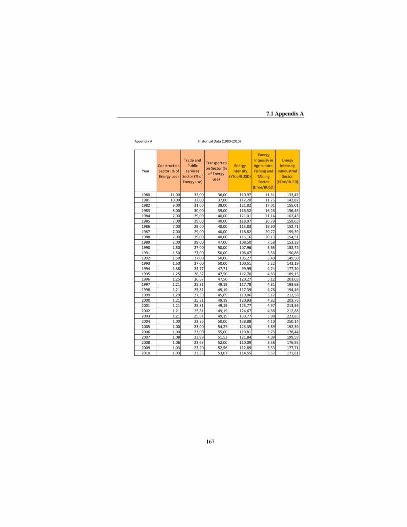
7.1 Appendix A
167
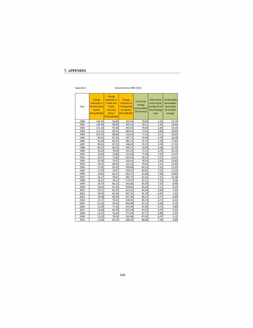
7. APPENDIX
168
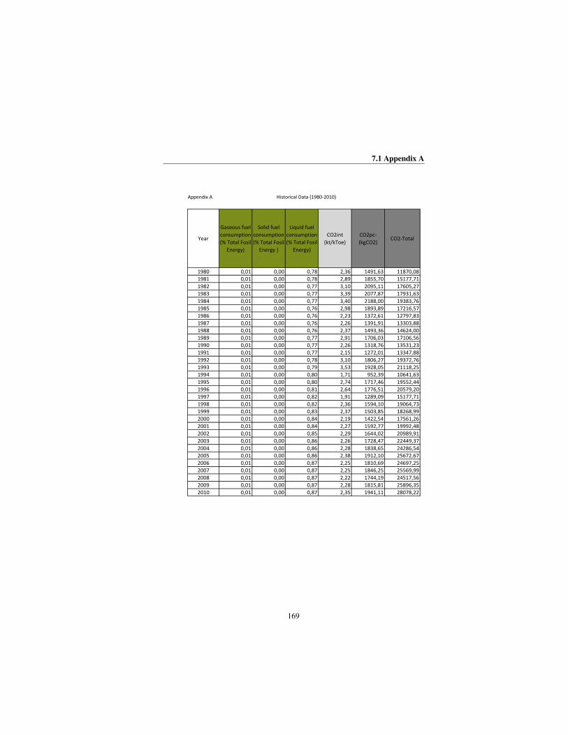
7.1 Appendix A
169

7. APPENDIX
170

7.2 Appendix B
7.2 Appendix B
Appendix B presents the outcomes of the model in the period 1980-2010. We use
this results in the model validation.
171

7. APPENDIX
172
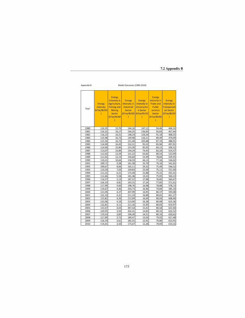
7.2 Appendix B
173
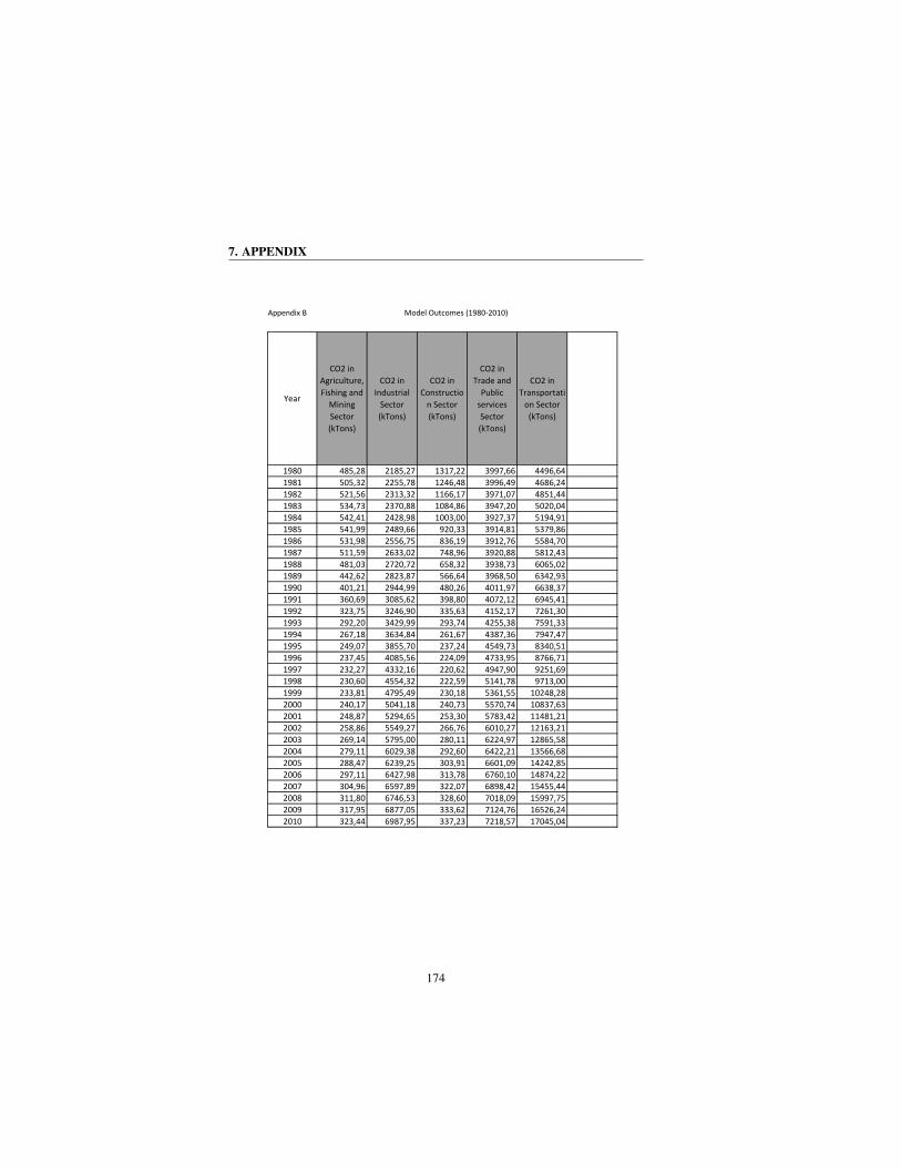
7. APPENDIX
174
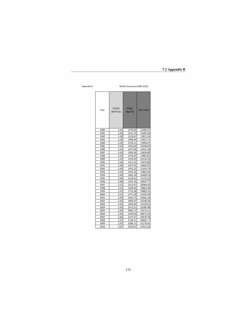
7.2 Appendix B
175

7. APPENDIX
176

7.3 Appendix C
7.3 Appendix C
Appendix C presents the outcomes of the model in the forecast period 2011-2025
for the four considered scenarios. We use these results in both decomposition ana-
lysis (Chapter 4) and EKC study (Chapter 5).
177

7. APPENDIX
178

7.3 Appendix C
179

7. APPENDIX
180

7.3 Appendix C
181
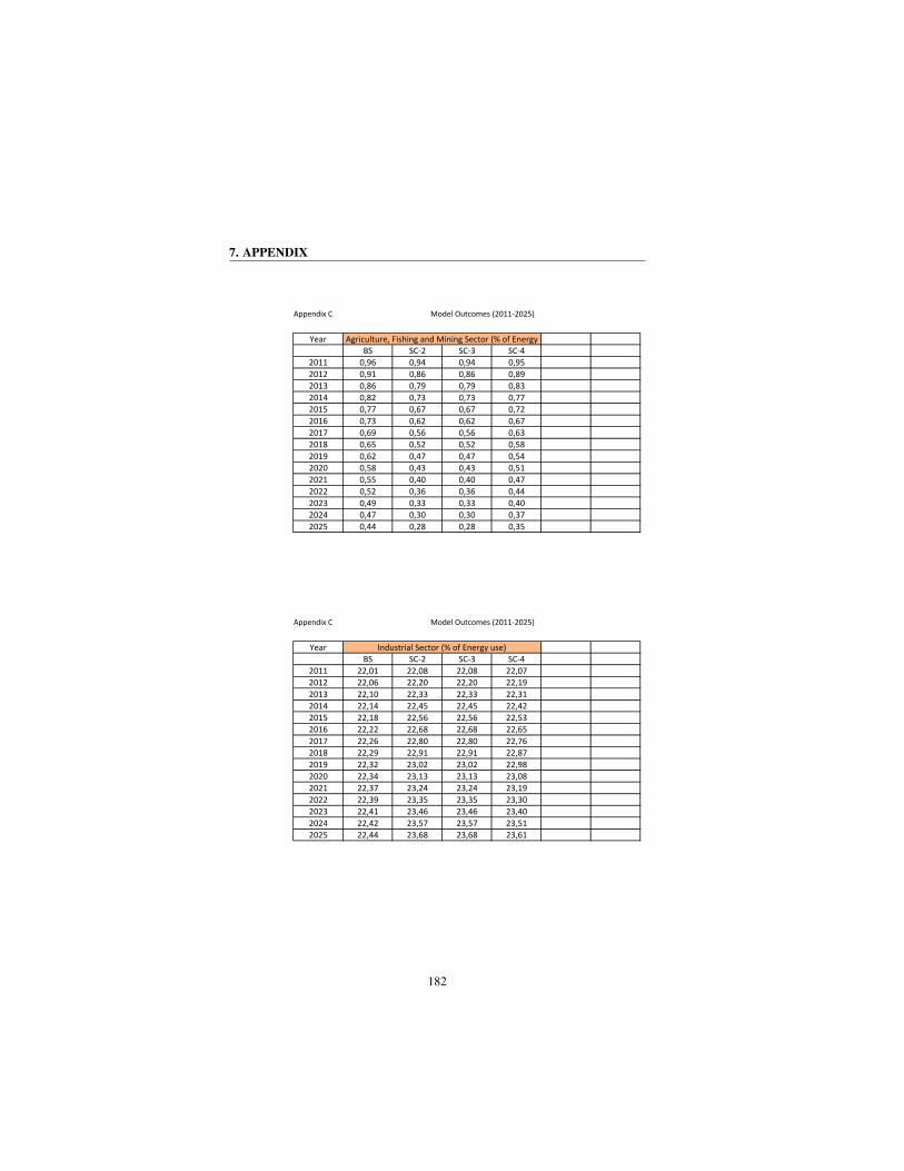
7. APPENDIX
182

7.3 Appendix C
183
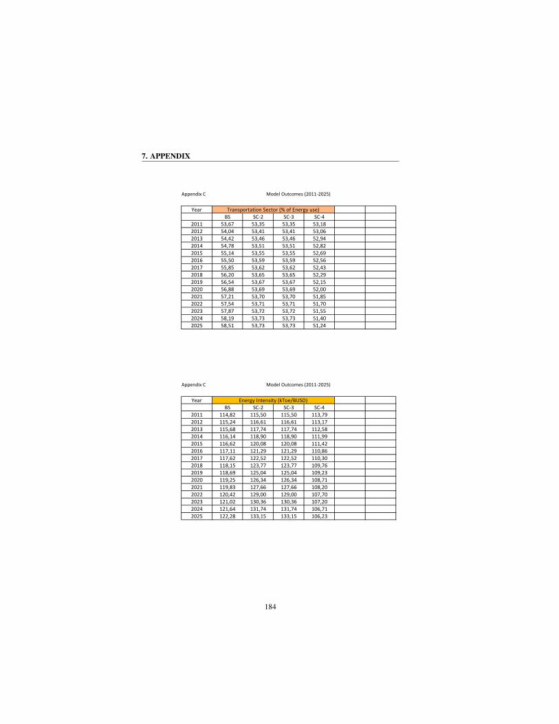
7. APPENDIX
184

7.3 Appendix C
185

7. APPENDIX
186

7.3 Appendix C
187

7. APPENDIX
188

7.3 Appendix C
189
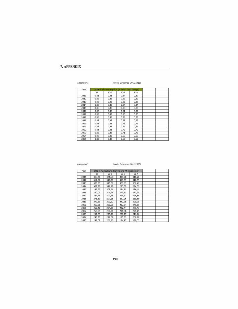
7. APPENDIX
190

7.3 Appendix C
191

7. APPENDIX
192

7.3 Appendix C
193
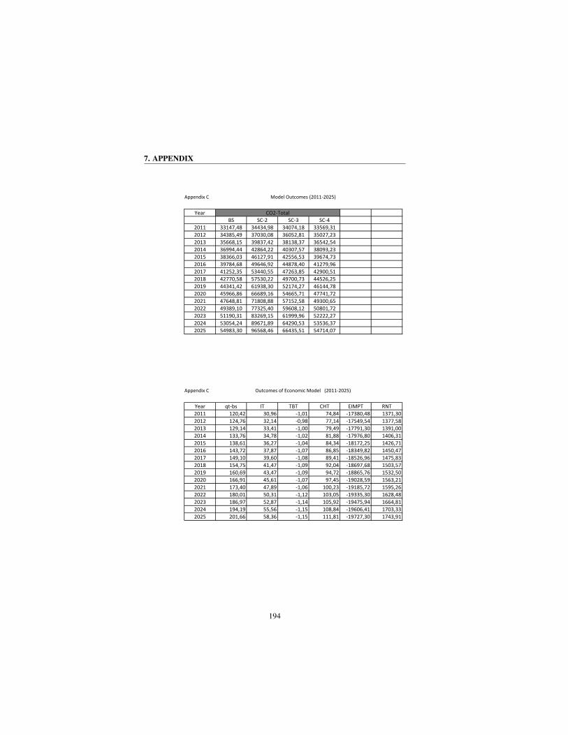
7. APPENDIX
194
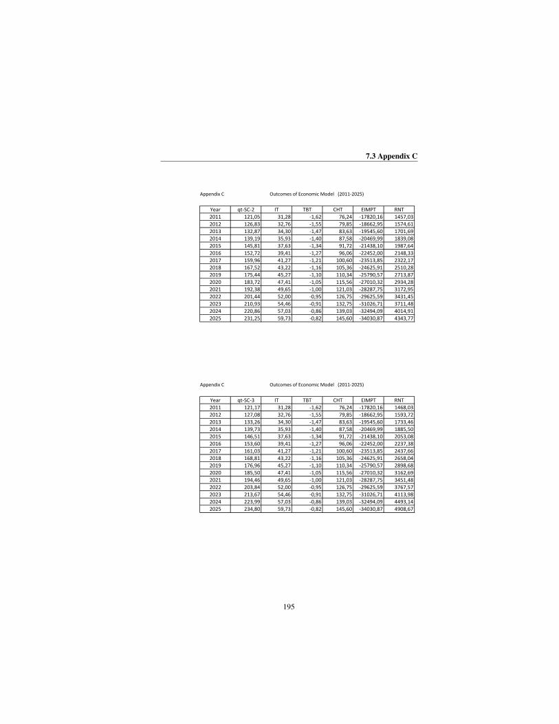
7.3 Appendix C
195
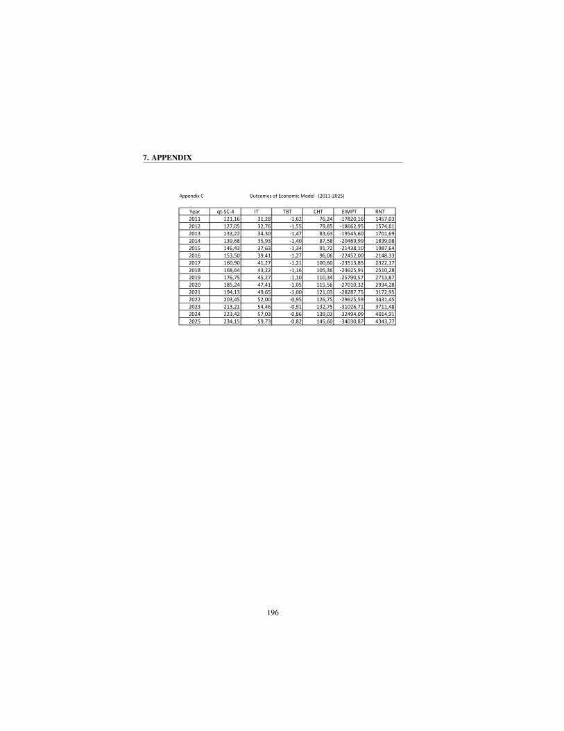
7. APPENDIX
196

7.4 Appendix D
7.4 Appendix D
Appendix D presents the outcomes of the LDMI analysis (Chapter 4) year by year
for the four considered scenarios in the period 1980-2025.
197

7. APPENDIX
198

7.4 Appendix D
199
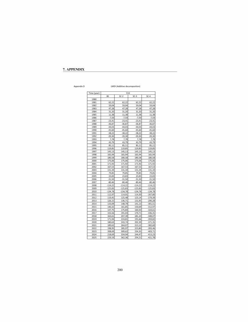
7. APPENDIX
200

7.4 Appendix D
201

7. APPENDIX
202
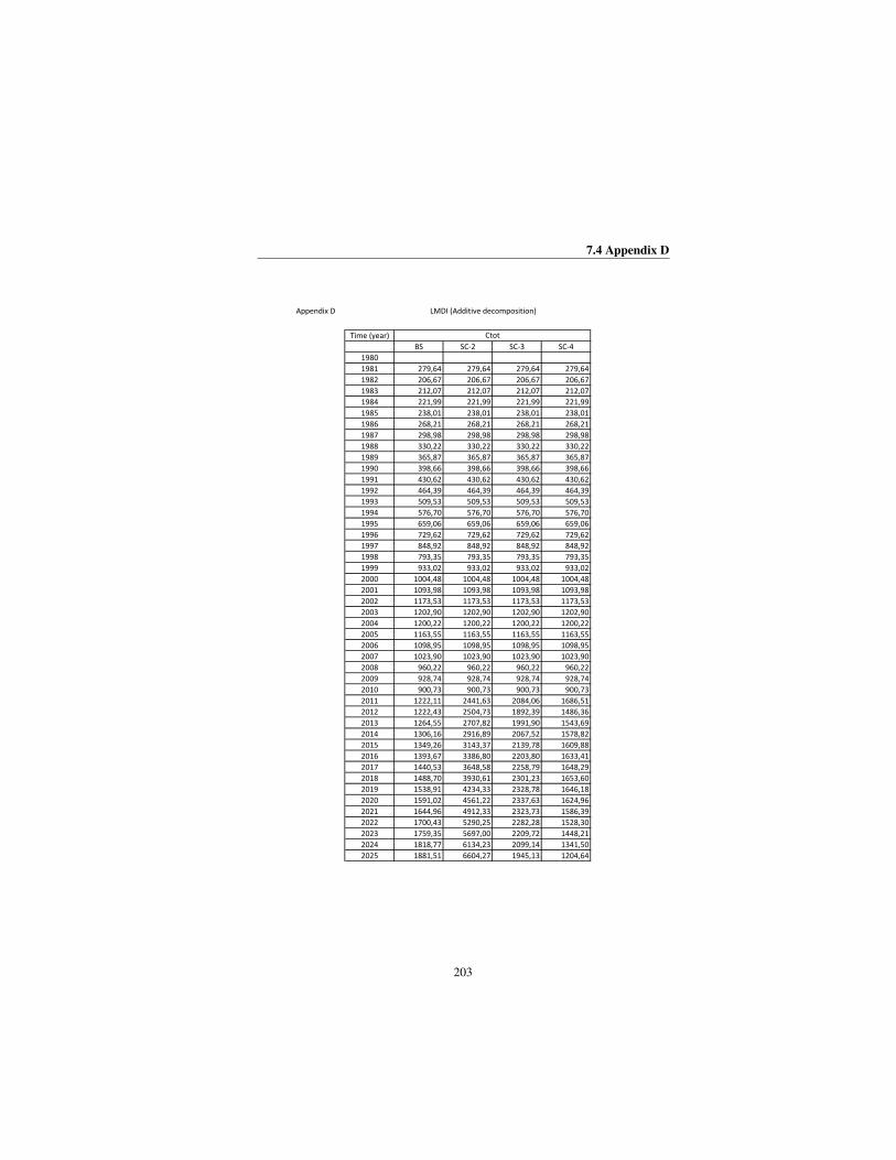
7.4 Appendix D
203
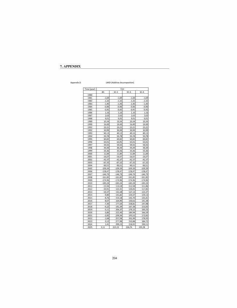
7. APPENDIX
204

7.5 Appendix E
7.5 Appendix E
Appendix E presents values of CO2-income elasticity for Ecuador (2011-2025).
Figure 5.5 in Chapter 5 is based on this data.
205

7. APPENDIX
206

7.6 Appendix F
7.6 Appendix F
Appendix F presents the programming of the model in Vensim platform. Note that
the programming is based on the equation system of Section 3.7 in Chapter 3.
207

7. APPENDIX
208

7.6 Appendix F
209

7. APPENDIX
210

7.6 Appendix F
211
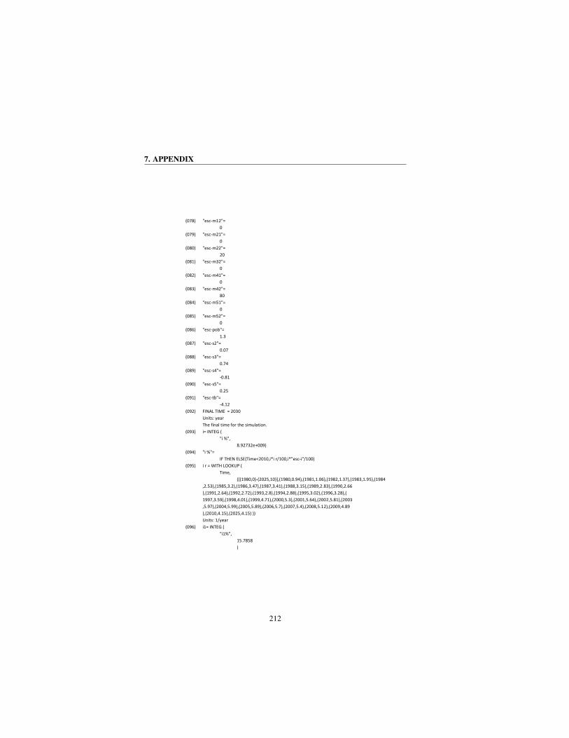
7. APPENDIX
212

7.6 Appendix F
213

7. APPENDIX
214
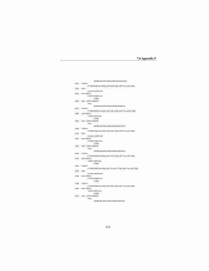
7.6 Appendix F
215

7. APPENDIX
216
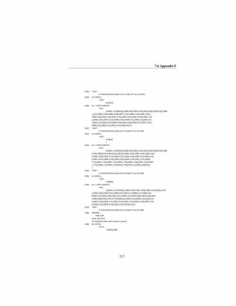
7.6 Appendix F
217

7. APPENDIX
218

7.7 Appendix G
7.7 Appendix G
Appendix G presents the outcomes of the Seemingly Unrelated Regression (SUR)
method that was used to solve the equation system in Section 3.7 in Chapter 3.
219
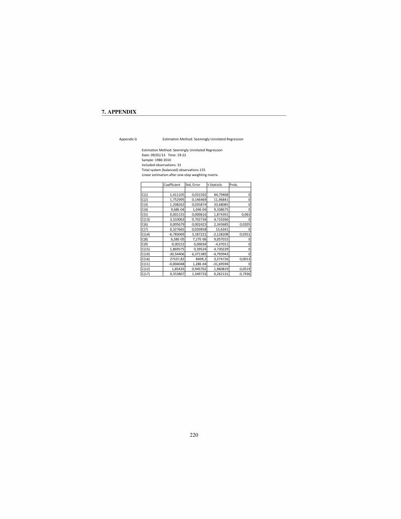
7. APPENDIX
220
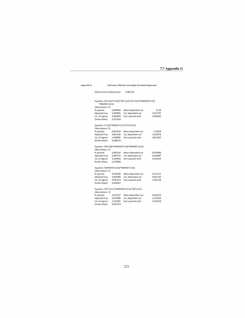
7.7 Appendix G
221

Bibliography
[1] Nickelback. When We Stand Together. http://www.youtube.com/
watch?v=B5VM5aq4rmY, 2011. i
[2] Arent D., Alison W., and Rachel G. The status and prospects of renewable
energy for combating global warming. Energy Economics: 33: 584–593,
2011. xv, 4, 5, 10, 66
[3] CONELEC (National Council for Electrification of Ecuador). Electri-
fication Master Plan 2009-2020. http://www.conelec.gob.ec/
documentos.php?cd=4171&l=1, 2009. xvi, 63, 64, 65, 67, 68
[4] Bruckner T., Chum H., Jager-Waldau A., Killingtveit A., Gutierrez-Negrın
L., Nyboer J., Musial W., Verbruggen A., 2011: Annex III: Cost Table.
In IPCC Special Report on Renewable Energy Sources Wiser R., Climate
Change Mitigation [Edenhofer O., Pichs-Madruga R., Sokona Y., Sey-
both K., Matschoss P., Kadner S., Zwickel T., Eickemeier P., Hansen G.,
Schlomer S., and von Stechow C. (eds)]. IPCC Special Report on Renew-
able Energy Sources and Climate Change Mitigation. Cambridge University
Press, Cambridge, United Kingdom and New York, NY, USA., 2011. xvi,
64, 67, 68
[5] Chien T. and Hu Jin-Li. Renewable energy: An efficient mechanism to
improve gdp. Energy Policy 36, 3045-3052, 2008. xvi, 72, 76, 78, 79, 80,
83, 152, 155
223
BIBLIOGRAPHY
[6] IPCC (Intergobernmental Panel on Climate Change). 2006 IPCC Guidelines
for National Greenhouse Gas Inventories, Prepared by the National Green-
house Gas Inventories Programme, Volume 2: Energy’. Cambridge Univer-
sity Press, 2006. xvi, 87, 88, 89, 90
[7] Islam N., Vincent J., and Panayotou T. Unveilingtheincome–environment
relationship: anexplorationintothedeterminantsofenvironmentalquality.
http://www.cid.harvard.edu/hiid/701.pdfS, 1999. xviii,
137
[8] Iglesias J., Carmona M., Golpe A., and Martin J.M. La curva de Kuznets
y la emission de CO2 en Espana, 1850-2008. Economıa Industrial, 2013.
xviii, 144
[9] EC (European Commission). Cimate action. The 2020 climate and energy
package’. http://ec.europa.eu/clima/policies/package/
index_en.htm, May 2014. 1
[10] Melillo Jerry M., Terese (T.C.) Richmond, and Gary W. Yohe. Highlights
of Climate Change Impacts in the United States: The Third National Cli-
mate Assessment. U.S. Global Change Research Program. U.S. Government
Printing Office. ISBN 9780160924033, 2014. 1
[11] United Nations (UN). Rio Declaration on Environment and Development
1992. Technical report, United Nations (UN), 1992. 2
[12] IEA (International Energy Agency). Clean Energy Progress Report. http:
//www.iea.org/publications/tcep_web.pdf, 2011. 4
[13] WEC (World Energy Council). 2010 Survey of Energy Resources.
http://www.worldenergy.org/documents/ser_2010_
report_1.pdf, 2010. 4
[14] Wiser R., Yang Z., Hand M., Hohmeyer O., Infield D., Jensen P. H., Nikolaev
V., O’Malley M., Sinden G., 2011: Wind Energy. In IPCC Special Report on
Renewable Energy Sources Zervos A., Climate Change Mitigation [Eden-
hofer O., Pichs-Madruga R., Sokona Y., Seyboth K., Matschoss P., Kadner
224
BIBLIOGRAPHY
S., Zwickel T., Eickemeier P., Hansen G., Schlomer S., and von Stechow
C. (eds)]. IPCC Special Report on Renewable Energy Sources and Cli-
mate Change Mitigation. Cambridge University Press, Cambridge, United
Kingdom and New York, NY, USA, 2011. 4, 5, 66
[15] Couture T., Cory K., Kreycik C., and Williams E. Policymaker’s Guide to
Feed-in Tariff Policy Design. National Renewable Energy Laboratory, U.S.
Dept. of Energy, 2010. 5
[16] Arvizu D., Balaya P., Cabeza L., Hollands T., Jager-Waldau A., Kondo M.,
Konseibo C., Meleshko V., Stein W., Tamaura Y., Xu H., 2011: Direct Solar
Energy. In IPCC Special Report on Renewable Energy Sources Zilles R.,
Climate Change Mitigation [Edenhofer O., Pichs-Madruga R., Sokona Y.,
Seyboth K., Matschoss P., Kadner S., Zwickel T., Eickemeier P., Hansen G.,
Schlomer S., and von Stechow C. (eds)]. IPCC Special Report on Renew-
able Energy Sources and Climate Change Mitigation. Cambridge University
Press, Cambridge, United Kingdom and New York, NY, USA., 2011. 5, 6
[17] Kammen D. Renewable Energy, Taxonomic Overview. En Cutler J. Cleve-
land (Ed.), Encyclopedia of Energy, Berkeley, Elsevier, 2004. 6
[18] Chum H., Faaij A., Moreira J., Berndes G., Dhamija P., Dong H., Gabrielle
B., Goss Eng A., Lucht W., Mapako M., Masera Cerutti O., McIntyre T.,
Minowa T., 2011: Bioenergy. In IPCC Special Report on Renewable En-
ergy Sources Pingoud K., Climate Change Mitigation [Edenhofer O., Pichs-
Madruga R., Sokona Y., Seyboth K., Matschoss P., Kadner S., Zwickel T.,
Eickemeier P., Hansen G., Schlomer S., and von Stechow C. (eds)]. IPCC
Special Report on Renewable Energy Sources and Climate Change Mitiga-
tion. Cambridge University Press, Cambridge, United Kingdom and New
York, NY, USA., 2011. 7, 8, 69
[19] Carriquiri M., Xiaodong D., and Govinda T. Second generation biofuels:
Economics and policies. Energy Policy 39: 4222–4234, 2011. 7
[20] REN 21 (Renewable Energy Policy Network for the 21st Century). Renew-
ables 2011 Global Status Report. Paris, REN 21 Secretariat, 2011. 8
225
BIBLIOGRAPHY
[21] A. Lewis, Estefen S., Huckerby J., Musial W., Pontes T., 2011: Ocean
Energy. In IPCC Special Report on Renewable Energy Sources Torres-
Martinez J. and, Climate Change Mitigation [Edenhofer O., Pichs-Madruga
R., Sokona Y., Seyboth K., Matschoss P., Kadner S., Zwickel T., Eickemeier
P., Hansen G., Schlomer S., and von Stechow C. (eds)]. IPCC Special Re-
port on Renewable Energy Sources and Climate Change Mitigation. Cam-
bridge University Press, Cambridge, United Kingdom and New York, NY,
USA., 2011. 8
[22] Goldstein B., Hiriart G., Bertani R., Bromley C., Gutierrez-Negrın L.,
Huenges E., Muraoka H., Ragnarsson A., Tester J., 2011: Geothermal En-
ergy. In IPCC Special Report on Renewable Energy Sources Zui V., Cli-
mate Change Mitigation[Edenhofer O., Pichs-Madruga R., Sokona Y., Sey-
both K., Matschoss P., Kadner S., Zwickel T., Eickemeier P., Hansen G.,
Schlomer S., and von Stechow C. (eds)]. IPCC Special Report on Renew-
able Energy Sources and Climate Change Mitigation. Cambridge University
Press, Cambridge, United Kingdom and New York, NY, USA., 2011. 8, 9
[23] Kriegler E. Comment. Energy Economics 33: 594–596, 2011. 11, 12
[24] R. Sims, Mercado P., Krewitt W., Bhuyan G., Flynn D., Holttinen H.,
Jannuzzi G., Khennas S., Liu Y., O’Malley M., Nilsson L. J., Ogden J.,
Ogimoto K., Outhred H., Ulleberg Ø., 2011: Integration of Renewable
Energy into Present van Hulle F., Future Energy Systems. In IPCC Spe-
cial Report on Renewable Energy Sources, Climate Change Mitigation [Ed-
enhofer O., Pichs-Madruga R., Sokona Y., Seyboth K., Matschoss P., Kad-
ner S., Zwickel T., Eickemeier P., Hansen G., Schlomer S., and von Stechow
C. (eds)]. IPCC Special Report on Renewable Energy Sources and Cli-
mate Change Mitigation. Cambridge University Press, Cambridge, United
Kingdom and New York, NY, USA, 2011. 11, 66
[25] IPCC (Intergobernmental Panel On Climate Change). Summary for Policy-
makers. in von Stechow C. and Edenhofer O. and Pichs-Madruga R. and
Sokona Y. and Seyboth K. and Matschoss P. and Kadner S. and Zwickel T.
226

BIBLIOGRAPHY
and Eickemeier P. and Hansen G. and Schlomer S.(Eds.), IPCC Special Re-
port on Renewable Energy Sources and Climate Change Mitigation. Cam-
bridge, Cambridge University Press, 2011. 11
[26] Lund H. and Mathiesen B. Energy system analysis of 100% renewable en-
ergy systems- The case of Denmark in years 2030 and 2050. Energy 34:
524– 531, 2009. 11
[27] Bayod-Rujula A. Future development of the electricity systems with distrib-
uted generation. Energy 34: 377-383, 2009. 12
[28] Ebinger J. and Vergara W. Climate Impacts on Energy Systems. Key Issues
for Energy Sector Adaptation. Energy Sector Management Assistance Pro-
gram (ESMAP). Technical report, Washington DC.,The World Bank, 2010.
12
[29] Bouffard F. and Kirschen D. Centralised and distributed electricity systems.
Energy Policy 36: 4504-4508, 2008. 12
[30] Nair N. and Zhang L. SmartGrid: Future networks for New Zealand power
systems incorporating distributed generation. Energy Policy 37: 3418–3427,
2009. 12
[31] Lindley D. The Energy Storage Problem. Nature. 463: 18-20, 2010. 12, 13
[32] Van’t Klooster S.A. and van Asselt M.B.A. Practicing the scenario-axis
technique. Futures 38 (1), 15-30, 2006. 13
[33] J.S. Armstrong. Principles of forecasting. A handbook for researchers and
practitioners. Springer science and business media, New York, New York,
2001. 13
[34] Agnolucci P., Ekins P. abd Iacopini G., Anderson K., Bows A., Mander
S., and S. Shackley. Different scenarios for achieving radical reduction
in carbon emissions: a decomposition analysis. Ecological Economics 68,
1652–1666, 2009. 13, 20
227

BIBLIOGRAPHY
[35] Linderoth H. Forecast errors in IEA-countries’ energy consumption. Energy
Policy 30, 53-61, 2002. 13, 14
[36] Winebrake J.J. and D. Savka. An evaluation of errors in US energy forecasts:
1982–2003. Energy Policy 34, 3475–3483, 2006. 13
[37] O’Neill B.C. and Desai M. Accuracy of past projections of US energy
consumption. Energy Policy 33 (8), 979-993, 1996. 14
[38] Pilavachi P.A., Dalamaga T., Rossetti di Valdalbero D., and Guilmot J.F.
Ex-post evaluation of European energy models. Energy Policy 36(5), 1726-
1735, 2008. 14
[39] H. de Jouvenel. A brief methodological guide to scenario building. Techno-
logical Forecasting and Social Change 65, 37–48, 2000. 14
[40] Nielsen S. K. and Karlsson K. Energy scenarios: a review of methods,
uses and suggestions for improvement. International Journal Global Energy
Issues 27 (3), 2007. 14, 21, 22, 95
[41] Middtun A. and Baumgartner T. Negotiating Energy Futures: The Politics
of Energy Forecasting. Energy Policy 14, 219-41, 1986. 14
[42] IPCC (Intergobernmental Panel on Climate-Change). 2006 IPCC Guidelines
for National Greenhouse Gas Inventories, Prepared by the National Green-
house Gas Inventories Programme’. Cambridge University Press, 2006. 16,
86, 94, 153, 154
[43] Pyle D. Data Preparation for Data Mining. Morgan Kaufmann Publishers,
Los Altos, California, 1999. 16
[44] Kotsiantis S., Kanellopoulos D., and Pintelas P. Data Preprocessing for Su-
pervised Leaning. International Journal of Computer Science, 2006, Vol 1
N. 2, pp 111-117, 2006. 17
[45] Hodrick R. and Prescott E. Postwar U.S. Business Cycles: an Empirical
Investigation. Carnegie-Mellon University; Discussion Papers 451, North-
western University, 1980. 17
228

BIBLIOGRAPHY
[46] Finn E. Kydland and Prescott E. Business Cycles: Real Facts and a Mon-
etary Myth. Quarterly Review 14 (2): 3–18, Federal Reserve Bank of Min-
neapolis, 1990. 17
[47] York R., Rosa E. A., and Dietz T. STIRPAT, IPAT and ImPACT: analytic
tools for unpacking the driving forces of environmental impacts. Ecological
Economics 46(3), 351–365, 2003. 18
[48] Commoner B. A Bulletin Dialogue on The Closing Circle. Response. Bul-
letin of the Atomic Scientists 28 (17), 42-56, 1972. 18
[49] Ehrlich P. R. and Holdren J.P. A Bulletin Dialogue on the Closing Circle:
Critique. One-Dimensional Ecology. Bulletin of the Atomic Scientists 28:16-
27, 1972. 18
[50] Y. Kaya. Impact of Carbon Dioxide Emission Control on GNP Growth:
Interpretation of Proposed Scenarios. Paper presented to the IPCC Energy
and Industry Subgroup, Response Strategies Working Group, Paris, (mimeo),
1990. 18, 20
[51] IPCC (Intergobernmental Panel On Climate Change). IPCC Special Reports.
Emissions Scenarios. Cambridge University Press, The Edinburgh Building
Shaftesbury Road, Cambridge CB2 2RU England, 2000. 18, 21
[52] Ang B.W. Decomposition analysis for policymaking in energy: which is the
preferred method? Energy Policy 32, 2004. 19, 112, 121, 126
[53] Steenhof P., Woudsma C., and Sparling E. Greenhouse gas emissions and
the surface transport of freight in Canada. Transportation Research Part
D-Transport and Environment 11 (5), 369–376, 2006. 19, 20
[54] Waggoner P.E. and Ausubel J.H. A framework for sustainability science: a
renovated IPAT identity. Proceedings of the National Academy of Sciences
99 (12), 7860-7865, 2002. 19
[55] Ang B.W. and Zhang F.Q. A survey of index decomposition analysis in
energy and environmental analysis. Energy 25, 1149-1176, 2000. 20, 115,
116, 118, 119, 120, 121
229

BIBLIOGRAPHY
[56] Sun J.W. Energy demand in the fifteen European Union countries by 2010
-A forecasting model based on the decomposition approach. Energy 26,
549–560, 2001. 20
[57] Sorrell S., Lehtonen M., Stapleton L., J. Pujol, and T. Champion. Decom-
posing road freight energy use in the United Kingdom. Energy Policy 37 (8),
3115-3129, 2009. 20
[58] Kwon T.H. A scenario analysis of CO2 emission trends from car travel:
Great Britain 2000–2030. Transport Policy 12 (2), 175–184, 2005. 20
[59] P. Steenhof. Decomposition for emission baseline setting in China’s electri-
city sector. Energy Policy 35 (1), 280–294, 2007. 20
[60] Van Notten P., Rotmans J., van Asselt M., and Rothman D. An updated
scenario typology. Futures 35 (5), 423-443, 2003. 21
[61] Silberglitt R., Hove A., and Shulman P. Silberglitt R. and Hove A. and
Shulman P. Technological Forecasting and Social Change 70 (4), 297-315,
2003. 21
[62] Alcamo J. Environmental Futures. The practice of environmental scenario
analysis. Developments in Integrated Environmental Assessment 2. Elsevier,
Amsterdam, the Netherlands, 2009. 21
[63] Borjeson L., Hojer M., Dreborg K., Ekvall T., and G. Finnveden. Scenario
types and techniques: towards a user’s guide. Futures 38, 723–739, 2006.
21
[64] Nakicenovic N., Alcamo J. abd Davis G., de Vries B., Fenham J., Gaffin
S., Gregory K., Grubler A., Jung T.-Y., Kram T., La Rovere E.L., Michaelis
L., Mori S., Morita T., Pepper W., Pitcher H., Price L., Riahi K., Reohrl
A., Rogner H.H., Sankovski A., Schlesinger M., Shukla P., Smith S., Swart
R., van Rooijen S., Victor N., and Dadi Z. Special report on emissions
scenarios. Working Group III, Intergovernmental Panel on Climate Change
(IPCC). Cambridge University Press, Cambridge, 2000. 21, 95, 161
230
BIBLIOGRAPHY
[65] Great Britain. Dept. of Energy. Economics and Statistics Division Great Bri-
tain. Dept. of Energy. Energy Forecasting Methodology Numero 29 de En-
ergy paper. Stationery Office, ISBN 0114106509, 9780114106508, 1978.
22
[66] Johansen L. A multi-sectoral study of economic growth. North-Holland Pub.
Co., 1974 - Business and Economics, 74. 22
[67] Toshihiko N. Energy-economic models and the environment. Progress in
Energy and Combustion Science 2004;30(4):417-475, 2004. 22
[68] Wei Y.M., Wu G., Liu L.C., and Fan Y. Progress in modeling for
energy-economy-environment complex system and its applications. Chinese
Journal of Management 2005;3(2):159-170, 2005. 23
[69] Grohnheit P. Economic interpretation of the EFOM model. Butterworth-
Heinemann Ltd-0140-9883/91/020143-10 1991, 1991. 23
[70] Van der Voort E., Donni E., Thonet C., Bois d’Enghien, Dechamps C., and
Guilmot J. F. Energy Supply Modelling Package EFOM 12 C Mark I -
Mathematical Description, CABAY,. Technical report, Commission of the
European Communities, 1984. 23
[71] Leontief W. Input-output economics. New York, Oxford University Press,
1966, 1966. 23
[72] Thijs Ten Raa. Input–output economics: theory and applications: featuring
Asian economies. World Scientific Publishing Co. Pte. Ltd., 2010. 23
[73] William H.M. Basic Theory of input-output analysis. Beijing: China Social
Sciences Press, 1980. 23
[74] Lazarus M., Heaps C., and von Hippel D. Methods for assessment of mit-
igation options Appendix IV: Mitigation Assessment Handbook. Technical
report, Stockholm Environment Institute and Tellus Institute, 1994. 24
231

BIBLIOGRAPHY
[75] Joost S. The Long–range energy alternatives planning model (LEAP) and
wood energy planning. http://www.rwedp.org/p_leap.html,
2004. 24
[76] Naughten B. Economic assessment of combined cycle gas turbines in Aus-
tralia some fffects of microeconomic reform and technological change. En-
ergy Policy 2003;31(3):225–245, 2003. 24
[77] Evasio L. Exploring energy technology perspectives. http://www.
etsap.org/markal/main.html, March 2004. 24
[78] Radzicki M.J. and Taylor R.A. Origin of System Dynamics: Jay W. For-
rester and the History of System Dynamics. U.S. Department of Energy’s
Introduction to System Dynamics, 2008. 25
[79] Meadows D.H., Meadows D.M., Randers J., and Behrems W. Limits to
Growth. New York, Universe books. ISBN 0-87663-165-0, 1972. 25
[80] Naill R.F., Gelanger S., Klinger A., and Petersen E. An analysis of cost
effectiveness of US energy policies to mitigate global warming. System Dy-
namics Review 8, 111-118, 1992. 26
[81] Nordhaus W. and Z Yang. A regional dynamic general-equilibrium model of
Alternative climate-change strategies. The American Economic Review 86,
741-765, 1996. 26
[82] Fiddaman Thomas S. Exploring policy with a behavioral climate-economy
model. System Dynamics Review. 18, 243-267, 2002. 26, 71
[83] Feng Y.Y., Chen S.Q., and Zhang L.X. System dynamics modeling for urban
energy consumption and CO2 emissions: a case study of Beijing, China.
Ecological Modelling 2013;252:44–52, 2012. 26
[84] A. Bassi and Baer A. Quantifying cross-sectoral impacts of investments in
climate change mitigation in Ecuador. Energy for Sustainable Development
13, 116-123, 2009. 26
232

BIBLIOGRAPHY
[85] System Dynamics Society. Introduction to System Dynamics. http://
www.systemdynamics.org/what-is-s/, January 2014. 26
[86] Garcıa J. Theory and Practical Exercises of System Dynamics. Spain. ISBN
84-607-9304-4, Legal Deposit B-4958-2003, 2011. 26, 72
[87] Forrester J.W. Urban Dynamics. Cambridge, MA: The MIT Press. Reprinted
by Pegasus Communications, 1969. 29, 30
[88] Kuznets P. and Simon P. Economic growth and income inequality. American
Economic Review 45, 1– 28, 1955. 31, 135
[89] Dasgupta S., Laplante B., Wang H., and Wheeler D. Confronting the
Environmental Kuznets Curve. Journal of Economic Perspectives 16 (1),
147–168, 2002. 32
[90] Anderson D. and Cavandish W. Dynamic simulation and environmental
policy analysis: beyond comparative statics and environmental Kuznets
curve. Oxford Economic Papers 53, 721– 746, 2001. 32, 40
[91] Beckerman W. Economic growth and the environment: whose growth?
Whose environment? Development 20, 481–496, 1992. 32, 138
[92] Shafik N. and Bandyopadhyay S. Economic Growth and Environmental
Quality: Time Series and Cross-Country Evidence. Background Paper for
the World Development Reportk. Technical report, The World Bank, Wash-
ington, DC, 1992. 32, 136
[93] Dinda S. Environmental Kuznets Curve Hypothesis: A Survey. Ecological
Economics 49 (2004) 431–455, 2004. 32, 34, 35, 38, 39, 40, 136, 137, 138,
139, 140, 142
[94] Gangadharan L. and Valenzuela M.R. Inter-relationships between income,
health and the environment: extending the Environmental Kuznets curve
hypothesis. Ecological Economics 36 (3), 513– 531, 2001. 33
[95] Dinda S., Coondoo D., and Pal M. Air quality and economic growth: an
empirical study. Ecological Economics 34 (3), 409– 423, 2000. 33
233

BIBLIOGRAPHY
[96] Grossman G.M. and Krueger A.B. Economic growth and the environment.
Quarterly Journal of Economics 110 (2), 353– 377, 1995. 33, 35
[97] de Bruyn S.M. and J.B. Opschoor. Developments in the throughput – income
relationship: theoretical and empirical observations. Ecological Economics
20, 255– 268, 1997. 33
[98] Sengupta R.P. CO2 emission–income relationship: policy approach for cli-
mate control. Pacific Asia Journal of Energy 7 (2), 207– 229, 1997. 33
[99] de Bruyn S.M., van den bergh J.C.J.M., and Opschoor J.B. Economic growth
and emissions: reconsidering the empirical basis of Environmental Kuznets
Curves. Ecological Economics 25, 161–175, 1998. 33
[100] Dijkgraaf E. and Vollebergh H.R.S. Growth and environment— is there a
Kuznets curve for carbon emissions? University of Geneva, 1998. 33, 37
[101] Stern D.I. and Common M.S. Is there an environmental Kuznets curve for
sulfur? Journal of Environmental Economics and Management 41 (2), 162–
178, 2001. 33
[102] Stern D.I., Common M.S., and Barbier E.B. Economic growth and environ-
mental degradation: a critique of the environmental Kuznets curve. World
Development 24, 1151– 1160, 1996. 33, 38
[103] Selden T. and Song D. Neoclassical growth, the J Curve for abatement, and
the inverted-U Curve for pollution. Journal of Environmental Economics
and management 29, 162– 168, 1995. 33, 142
[104] Arrow K., Bolin B., Costanza R., Folke C., Holling C.S., Janson B., Levin
S., K. Maler, Perrings C., and D. Pimental. Economic growth, carrying
capacity, and the environment. Science 15, 91– 95 (reprint in Ecological
Economics), 1995. 34, 38
[105] Dinda S. Economic growth with environmental and physical capital: a con-
vergence approach. Mimeo, 2003. 34
234
BIBLIOGRAPHY
[106] Ekins P. Economic Growth and Environmental Sustainability. 182– 214
(chap. 7), 1998. 34, 35
[107] Gruver G.W. Optimal investment in pollution control capital in a neoclas-
sical growth context. Journal of Environmental Economics and Management
5, 165– 177, 1976. 34
[108] Zang H. The stability of the Kuznets Curve: some further evidence. Applic-
ation of Economics Letters 5, 131– 133, 1998. 34
[109] Panayotou T. Demystifying the environmental Kuznets curve: turning a
black box into a policy tool. Environment and Development Economics 2,
465– 484, 1997. 34, 35, 38
[110] Ezzati M., Singer B.H., and D.M. Kammen. Towards an integrated frame-
work for development and environmental policy: the dynamics of Environ-
mental Kuznets Curves. World Development 29 (8), 1421–1434, 2001. 35,
142
[111] Hung M.F. and Shaw D. TEconomic growth and the Environmental Kuznets
Curve in Taiwan: a simultaneity model analysis. Department of Economics,
National Cheng-Chi University. Mimeo, 2002. 35
[112] O’Neill R.V., Kahn J.R., Duncan J.R., Elliott S., Efroymson R., Cardwell
H., and D.W. Jones. Economic growth and sustainability: a new challenge.
Ecological Applications 6 (1), 23–24, 1996. 35
[113] Kaufmann R.K., Davidsdottir B., Garnham S., and P. Pauly. The determ-
inants of atmospheric SO2 concentrations: reconsidering the environmental
Kuznets curve. Ecological Economics 25, 209– 220, 1998. 35
[114] Dinda S. A theoretical basis for Environmental Kuznets Curve. Economic
Research Unit, Indian Statistical Institute, Kolkata. Mimeo, 2002. 36, 141,
142
[115] Tisdell C. Globalisation and sustainability: environmental Kuznets curve
and the WTO. Ecological Economics 39, 185–196, 2001. 36
235

BIBLIOGRAPHY
[116] Koop G. and Tole L. Is there an environmental Kuznets curve for deforesta-
tion? Journal of Development Economics 58, 231– 244, 1999. 36
[117] Taskin F. and O. Zaim. Searching for a Kuznets Curve in environmental
efficiency using kernel estimation. Economics Letters 68, 217– 223, 2000.
37
[118] Halkos G.E. and Tsionas E.G. Environmantal Kuznets Curves: Bayesian
evidence from switching regime models. Energy Economics 23, 191– 210,
2001. 37
[119] Bartoszezuk P., Ma T., and Y. Nakamari. Environmental Kuznets curve for
some countries—regression and agent-based approach. Japan Advance In-
stitute of science and Technology (mimeo), 2001. 37
[120] Perman R. and Stern D.I. The Environmental Kuznets Curve: implications
of non-stationarity. Australian National University. Mimeo, 1999. 37
[121] Coondoo D. and S Dinda. Causality between income and emission: a coun-
try group-specific econometric analysis. Ecological Economics 40 (3), 351–
367, 2002. 37
[122] Ansuategi A., Barbier E., and Perrings C. The Environmental Kuznets Curve.
In: van den Bergh, J.C.J.M., Hofkes, M.W. (Eds.). Theory and Implementa-
tion of Sustainable Development Modelling. Kluwer Academic, Dordrecht,
1998. 37
[123] Copeland B.R. and Taylor M.S. Trade and environment: a partial synthesis.
American Journal of Agricultural Economics 77, 765– 771, 1995. 37, 140
[124] Suri V. and D. Chapman. Economic growth, trade and the environment:
implications for the environmental Kuznets curve. Ecological Economics
25, 195– 208, 1998. 37
[125] Agras J. and Chapman D. A dynamic approach to the Environmental
Kuznets Curve hypothesis. Ecological Economics 28 (2), 267– 277, 1999.
37
236
BIBLIOGRAPHY
[126] Fare R., Grosskopt S., and O. Zaim. An index number approach to meas-
uring environmental performance: an Environmental Kuznets Curve for the
OECD countries, (mimeo). Department of economics, Oregon State Univer-
sity, USA, 2001. 37
[127] Grossman G.M. and Krueger A.B. The inverted-U: what does it mean? En-
vironment and Development Economics 1 (2), 119–122, 1996. 37
[128] Dinda S. A note on global EKC in case of CO2 emission. Economic Re-
search Unit, Indian Statistical Institute, Kolkata. Mimeo, 2001. 37
[129] Cole M.A., Rayner A.J., and Bates J.M. The Environmental Kuznets Curve
: an empirical analysis. Environment and Development. Economics 2, 401–
416, 1997. 38
[130] John A., Pecchenino R., Schimmelpfenning D., and Schreft S. Short-lived
agents and the long-lived environment. Journal of Public Economics 58,
127– 141, 1995. 38
[131] Grossman G.M. and Krueger A.B. Environmental impacts of the North
American Free Trade Agreement. NBER. Working paper 3914, 1991. 38,
114, 136, 137, 139
[132] Vukina T., Beghin J.C., and Solakoglu E.G. Transition to markets and the
environment: effects of the change in the composition of manufacturing out-
put. Environment and Development Economics 4 (4), 582– 598, 1999. 38,
139
[133] Xiaoli H. and Chatterjee L. Impact of growth and structural change on CO2
emissions of developing countries. World Development 25 (3), 395–407,
1997. 38
[134] Lucas R.E.B., Wheeler D., and Hettige H. Economic development, envir-
onmental regulation and the international migration of toxic industrial pol-
lution: 1960 – 1988. In: Low P. (Ed.) International Trade and the Environ-
ment, World Bank discussion paper 159, 67– 87, 1997. 38
237
BIBLIOGRAPHY
[135] Komen R., Gerking S., and Folmer H. Income and environmental R and D:
empirical evidence from OECD countries. Environment and Development
Economics 2, 505–515, 1997. 39, 139
[136] Smulder S. and Bretschger L. Explaining Environmental Kuznets Curves:
how pollution induces policy and new technologies. Center for Economic
Research working paper No. 2000- 95, Tilburg University, 2000. 39
[137] Lindmark M. An EKC-pattern in historical perspective: carbon dioxide
emissions, technology, fuel prices and growth in Sweden 1870– 1997. Eco-
logical Economics 42, 333– 347, 2002. 39
[138] Labys W.C. and Wadell L.M. Commodity lifecycles in US materials de-
mand. Resources Policy 15, 238–252, 1989. 39
[139] Pasche D. and Markus D. Technical progress, structural change, and the
environmental Kuznets curve. Ecological Economics 42, 381– 389, 2002.
40
[140] Munasinghe M. Is environmental degradation an inevitable consequence
of economic growth: tunneling through the environmental Kuznets curve.
Ecological Economics 29, 89– 109, 1999. 40, 141
[141] Robalino-Lopez A., Garcıa-Ramos J.E., Mena-Nieto A., and Golpe A. Sys-
tem dynamic modelling and the environmental Kuznets curve in Ecuador
(1980-2025). Energy Policy 67 (2014) 923-931, 2013. 42
[142] Robalino-Lopez A., Mena-Nieto A., and Garcıa-Ramos J.E. System dy-
namics modeling for renewable energy and CO2 emissions: A case study of
Ecuador. Energy for Sustainable Development 20 (2014) 11-20, 2014. 42
[143] Robalino-Lopez A., Mena-Nieto A., Garcıa-Ramos J.E., and Golpe A.
“Studying the relationship between economic growth, CO2 emissions, and
the environmental Kuznets curve in Venezuela (1980–2025)”. Renewable
and Sustainable Energy Reviews 41 (2015) 602–614, 2015. 42
238
BIBLIOGRAPHY
[144] Stock J. H. and Watson M. W. A simple estimator of cointegrating vectors
in higher order integrated systems. Econometrica 61, 783-820, 2010. 42,
149, 151, 159
[145] Jaunky V. C. The CO2 emissions-income nexus: Evidence from rich coun-
tries. Energy Policy, 39 (3), 1228-1240, 2011. 42, 143, 145, 146, 149, 152,
159
[146] WB (World Bank). Data, statistics and National referents-Ecuador. http:
//data.worldbank.org/country/ecuador, July 2012. 45, 46,
47, 48, 56, 72, 85, 86, 164
[147] CI (Conservation International). Megadiversity: The 17 Biodiversity
Superstars. http://www.conservation.org/documentaries/
Pages/megadiversity.aspx, March 2012. 45
[148] TCELDF (The Community Environmental Legal Defense Fund). About the
New Constitution 2008. http://www.Celdf.org, October 2011. 45,
47
[149] UNDP (United Nations Development Program). Human Development Re-
port 2011. United Nations Development Programme (UNDP), ISBN:
9780230363311, 2012. 45
[150] IM (IndexMundi). IndexMundi. http://www.indexmundi.com,
April 2014. 45, 48
[151] WB (World Bank). Data, statistics and National referents-Ecuador. http:
//data.worldbank.org/country/ecuador, April 2014. 45, 46,
48, 153
[152] BCE (Ecuadorian Central Bank). BCE indicators homepage. http://
www.bce.fin.ec/indicador.php, March 2012. 46, 72, 164
[153] IEA (International Energy Agency). Data Services homepage. http://
www.iea.org/, 2013. 46, 72, 164
239

BIBLIOGRAPHY
[154] A. Mosquera-Rodrıguez. Policies and Strategies for Changing the Energy
Matrix in Ecuador. Ministry of Electricity and Renewable Energy, Ecuador,
2008. 48, 52, 53, 54, 55, 62, 85, 97
[155] UN (United Nations). ST/ESA/STAT/SER.M/4/Rev.4. UNITED NATIONS
PUBLICATION, ISBN: 978-92-1-161518-0, 2008. 49
[156] IPCC (Intergobernmental Panel On Climate Change). Synthesis Report.
Contribution of Working Groups I, II, and III to the Fourth Assessment Re-
port of the Intergovernmental Panel on Climate Change’. Cambridge Uni-
versity Press, 2007. 58, 153
[157] CONELEC (National Council for Electrification of Ecuador). National
Council for Electrification (Consejo Nacional de Electrificacion). Treatment
for energy produced from non-conventional renewable energy resources
(CONELEC regulation no. 004/11). http://www.conelec.gob.ec,
2011. 62, 63
[158] Aquaculture MAG (Ministry of Agriculture, Livestock and Fisheries
of Ecuador). Major crops of Ecuador, total cropped area, historical
series 2000–2011. http://servicios.agricultura.gob.ec,
Dec 2011. 63
[159] MEER (Ministry of Electricity and Renewable Energy of Ecuador). Flagship
projects. http://www.energia.gob.ec, Dec 2011. 63, 65, 67
[160] ANCUPA (Area national oil palm. Ecuador Association of African
Palm Growers). Statistics. http://www.ancupa.com, 2013. 63
[161] USDA (United States Department of Agriculture). Ecuador 2011 biofuels
(biodiesel, biotethanol, biomass) sector policy development and outlook.
http://gain.fas.usda.gov., 2011. 63
[162] Neira D., Van Den Berg B., and De la Torre F. The Clean Development
Mechanism in Ecuador: A rapid diagnosis of the challenges and opportun-
ities in the Carbon Market. Interamerican Development Bank, 2006. 63
240

BIBLIOGRAPHY
[163] CEPAL (Comision Economica para America Latina y el Caribe). PROJECT
OLADE/CEPAL/GTZ: Study for the Environmental Assessment of the Bina-
tional Geothermal Projec Tufino-Chiles-Cerro Negro, LC/R. CEPAL, 2010.
64
[164] CONELEC (National Council for Electrification of Ecuador). National stat-
istics. http://www.conelec.gob.ec/documentos.php?cd=
4171&l=1, 2009. 64, 67
[165] CIE (Corporation for the Energy Research). Solar Atlas of Ecuador purposes
Electricity Generation. http://www.conelec.gob.ec/archivos_
articulo/Atlas.pdf, 2008. 65
[166] Taylor D. Wind Energy. En Godfrey Boyle (Ed.), Renewable Energy: Power
for a sustainable future. Cambridge, Oxford University Press, The Open
University, 2011. 66
[167] Caspary G. Gauging the future competitiveness of renewable energy in
Colombia. Energy Economics, 31: 443-449, 2009. 67
[168] Bahrman S., C. Lenker, and Michalek J. A Model Based Approach to Ana-
lyze the Effects of Automotive Air Emissions Policy on Consumers, Produ-
cers, and Air Quality. Eco Design and Manufacturing, 2007. 71
[169] Kaya Y. and Yokobori K. Environment, Energy, and Economy: strategies for
sustainability. Conference on Global Environment, Energy, and Economic
Development (1993 : Tokyo, Japan)., 1993. 72, 155
[170] Forrester J. Industrial Dynamics. Pegasus Communications, 1961. 72
[171] Vensim. Simulation environment window. Version PLE. http://www.
vensim.com/, October 2011. 72
[172] INEC (Ecuadorian Institute of Statistics and Censuses). National statistics.
http://www.inec.gov.ec, March 2012. 72, 164
241
BIBLIOGRAPHY
[173] Hodrick R. and Prescott E. Postwar U.S. Business Cycles: An Empirical
Investigation . Journal of Money, Credit and Banking, Vol. 29, No. 1 (Feb.,
1997), pp. 1-16, 1997. 72, 73, 74
[174] Alcantara V. and Padilla E. Analysis of CO2 and its explanatory factors in
the different areas of the world. Technical report, Universidad Autonoma de
Barcelona, Department of Economics Applied, Spain, 2005. 72
[175] Mena-Nieto A., Menaca C., Barrero A., and Bellido M. Application of the
system dynamics methodology for modeling and simulation of the green-
house gas emissions in Cartagena de Indias (Colombia). In: AEIPRO, editor.
Selected proceedings fromthe 13th international congress on project engin-
eering. Spain: Badajoz; 2009. p. 260–77, 2009. 72
[176] Begueri G. System Dynamics: A New Approach. Technical report, Univer-
sidad Nacional de San Juan, Argentina, 2001. 72
[177] Radzicki M.J. and Tauheed L. In Defense of System Dynamics: A Response
to Professor Hayden . Journal of Economic Issues 43 (4), 1043-1061, 2009.
72
[178] Tan B., Anderson E.G.Jr., Dyer J.S., and Parker G.G. Evaluating system
dynamics models of risky projects using decision trees: alternative energy
projects as an illustrative example. System Dynamics Review 26 (1), 1-17,
2010. 72
[179] Rowland D. Demographic methods and concepts, chap 2, population growth
and decline. Oxford University PressOxford University Press; 2003, 2003.
74, 91
[180] Jin Y., Yumi T., Tatsuya T., Shigehide S., and Kei ichi T. Mathematical
equivalence of geometric mean fitness with probabilistic optimization under
environmental uncertainty. Ecol Model 2009;220:26112617, 2009. 74, 91
[181] Zellner A. An Efficient Method of Estimating Seemingly Unrelated Regres-
sions and Tests for Aggregation Bias. Journal of the American Statistical
Association, Vol. 57, No. 298, 1962. 74, 82
242
BIBLIOGRAPHY
[182] StataCorp LP. StataCorp LP. http://www.stata.com/, 2012. 74
[183] Chien T. and Hu J.L. Renewable energy and macroeconomic efficiency of
OECD and non-OECD economies. Energy Policy 35, 3606–3615, 2007. 75,
76, 82
[184] Hu J.L. and Kao C.H. Efficient Energy-saving Targets for APEC Economies.
Energy Policy 35: 373–382, 2007. 75
[185] Hu J.L. and Wang S.C. Total-factor energy efficiency of regions in China.
Energy Policy 34 (17), 3206–3217, 2006. 75
[186] Schneider U.A. and McCarl B.A. Economic potential of biomass based
fuels for greenhouse gas emission mitigation. Environmental and Resource
Economics 24, 291–312, 2003. 75
[187] Dowaki K. and Mori S. Biomass energy used in a sawmill. Applied Energy
80, 327–339, 2005. 75
[188] Caputo A. Economics of biomass energy utilization in combustion and gas-
ification plants: effects of logistic variables. Biomass and Bioenergy 28,
35–51, 2005. 75
[189] Abulfotuh F. Energy efficiency and renewable technologies: the way to
sustainable energy future. Desalination 209, 275–282, 2007. 75
[190] Lund P.D. Effectiveness of policy measures in transforming the energy sys-
tem. Energy Policy 35, 627–639, 2007. 75
[191] REN 21 (Renewable Energy Policy Network for the 21st Century). Renew-
ables 2012 Global Status Report. Paris, REN 21 Secretariat, 2012. 76
[192] Domac J., Richards K., and Risovic S. Socio-economic drivers in imple-
menting bioenergy projects. Biomass and Bioenergy 28, 97–106, 2005. 76,
82
243
BIBLIOGRAPHY
[193] Mack Ott. National Income Accounts. Technical report, The Concise En-
cyclopedia of Economics. 2008. Library of Economics and Liberty. 12 May
2014., 2008. 77
[194] Cancelo M. and Dıaz M. CO2 emissions and economic growth in EU coun-
tries. Journal of International Development Economic Research. Technical
report, Universidad de Santiago de Compostela, Spain. JEL classification:
O13, O14, O52., 2002. 86
[195] Abulfotuh F. Simple versus Complex Models: Evaluation, Accuracy, and
Combining. Mathematical Population Studies 5: 281-90, 1995. 93
[196] Campbell P. Evaluating Forecast Error in State Population Projections Using
Census 2000 Counts. Population Division Working Paper Series No. 57.
Washington, D.C.: U. S. Census Bureau, 2002. 93
[197] Hyndman R. and Koehler A. Another Look at Measures of Forecast Accur-
acy. International Journal of Forecasting 22: 679-688, 2006. 93
[198] Isserman A. The Accuracy of Population Projections for Subcounty Areas.
Journal of the American Institute for Planners 43: 247-59, 1977. 93
[199] Miller E.R. Evaluation of the 1990 School District Level Population Estim-
ates Based on the Synthetic Ratio Approach. Population Division Working
Paper No. 54. Washington D.C.: US Census Bureau, 2001. 93
[200] Murdock S., Leistritz L., Hamm R., Hwang S., and Parpia B. An Assessment
of the Accuracy of a Regional Economic-Demographic Projection Model.
Demography 21: 383- 404, 1984. 93
[201] Rayer S. Population Forecast Accuracy: Does the Choice of Summary
Measure of Error Matter? Population Research and Policy Review 26: 163-
184, 2007. 93
[202] Sink L. Race and Ethnicity Classification Consistency between the Census
Bureau and the National Center for Health Statistics. Population Division
Working Paper No. 17. Washington, D.C.: U.S. Census Bureau, 1997. 93
244
BIBLIOGRAPHY
[203] Smith S. Tests of Accuracy and Bias for County Population Projections.
Journal of the American Statistical Association 82: 991-1003, 1987. 93
[204] Smith S. and Sincich T. On the Relationship Between Length of Base Period
and Population Forecast Errors. Journal of the American Statistical Associ-
ation 85: 367-75, 1990. 94
[205] Smith S. and Sincich T. Evaluating the Forecast Accuracy and Bias of Al-
ternative Projections for States. International Journal of Forecasting 8: 495-
508, 1992. 94
[206] Smith S., Tayman J., and Swanson D.A. State and Local Population Pro-
jections: Methodology and Analysis. New York: Kluwer Academic/Plenum
Publishers, 2001. 94
[207] Tayman J., Schafer E., and Carter L. The Role of Population Size in the De-
termination of Population Forecast Errors: An Evaluation using Confidence
Intervals for Subcounty Areas. Population Research and Policy Review 17:
1-20, 1998. 94
[208] Wilson T. The Forecast Accuracy of Australian Bureau of Statistics National
Population Projections. Journal of Population Research 24 (1): 91-117,
2007. 94
[209] Holmes H.H. Interpreting global energy and emission scenarios: methods
for understanding and communicating policy insights. Doctoral dissertation,
Stanford University, 2007. 95
[210] Hoekstra R. and Van der Bergh J.C.J.M. Comparing structural and index
decomposition analysis. Energy Economics 25 (1), 39–64, 2003. 112, 125
[211] Ang B.W. Decomposition analysis applied to energy. In: C.J. Cleveland,
Editor, Encyclopedia of Energy, Elsevier, Amsterdam, pp. 761–769, 2004.
112, 113
245

BIBLIOGRAPHY
[212] Hatzigeorgiou E., Polatidis H., and Haralambopoulos D. A decomposition
analysis and comparison of results using the Arithmetic Mean Divisia Index
and Logarithmic Mean Divisia Index techniques. Energy 33 (3), 492-499,
2008. 112
[213] Zhou P. and Ang B.W. CO2 emissions: a production-theoretical approach.
Energy Economics 30, 1054-1067, 2008. 112
[214] Proops J., Faber M., and Wagenhals G. Reducing CO2 emissions. A compar-
ative Input-Output study for Germany and the UK. Springer-Verlag, Berlin,
1993. 113, 114
[215] Ang B.W. Decomposition of industrial energy consumption. The energy
intensity approach. Energy Economics, 16(3), pp. 163-174, 1994. 115, 117,
118, 119
[216] Ang B.W. The LMDI approach to decomposition analysis: a practical guide.
Energy Policy 33 (2005) 867–871, 2005. 120, 126
[217] Ang B.W., Liu F.L., and Chew E.P. Perfect decomposition techniques in
energy and environmental analysis. Energy Policy 31, 1561–1566, 2003.
120
[218] Rose A. and Chen C.Y. Sources of change in energy use in the US economy,
1972-1982: a structural decomposition analysis. Resources and Energy, 13,
1991. 121
[219] Rose A. and Casler S. Input-Output structural decomposition analysis: a
critical appraisal. Economic Systems Research, 1996. 121
[220] Hoekstra R. and van den Bergh J.C.J:M. Structural decomposition analysis
of physical flows in the economy. Environmental and Resource Economics,
2002. 122, 123, 124, 125
[221] Miller R.E and Blair P.D. Input-Output analysis: foundations and exten-
sions. Prentice-Hall, Englewood-Cliffs, New Jersey, 1985. 123
246

BIBLIOGRAPHY
[222] UN Department of Economics and Social Affairs. Handbook of Input-
Output Table Compilation and Analysis. Studies in Methods – Handbook
of National Accounting: Series F. United Nations, NY., 1999. 124
[223] Panayotou T. Empirical tests and policy analysis of environmental degrad-
ation at different stages of economic development. ILO, Technology and
Employment Programme, Geneva, 1993. 136
[224] Pezzey J.C.V. Economic analysis of sustainable growth and sustainable de-
velopment. Environment Department working paper 15, 1989. 138
[225] Selden T. and Song D. Environmental quality and development: is there
a Kuznets Curve for air pollution emissions? Journal of Environmental
Economics and management 27, 147– 162, 1994. 138, 142
[226] Baldwin R. Does sustainability require growth? In: Goldin, I., Winters,
L.A. (Eds.). The Economics of Sustainable Development. Cambridge Univ.
Press, Cambridge, UK, pp. 19–47, 1995. 138
[227] Roca J. Do individual preferences explain Environmental Kuznets Curve?
Ecological Economics 45 (1), 3– 10, 2003. 138
[228] Carson R.T., Jeon Y., and McCubbin D.R. The relationship between air
pollution emissions and income : US data. Environment and Development
Economics 2, 433– 450, 1997. 138
[229] Chaudhuri S. and Pfaff A. Household income, fuel choice, and indoor air
quality: micro-foundations of an Environmental Kuznets Curve. Economics
Department, Columbia University. Mimeo, 1998. 138
[230] McConnell K.E. Income and the demand for environmental quality. Envir-
onment and Development Economics 2, 383– 399, 1997. 138
[231] Shafik N. Economic development and environmental quality: an economet-
ric analysis. Oxford Economic Papers 46, 1994. 138
247
BIBLIOGRAPHY
[232] Birdsall N. and Wheeler D. Trade policy and industrial pollution in Latin
America: where are the pollution havens? Journal of Environment and
Development 2, 137–149, 1993. 139
[233] Lee H. and Roland-Holst D. The environment and welfare implications of
trade and tax policy. Journal of Development Economics 52 (1), 65– 82,
1997. 139
[234] Jones L.E. and Rodolfo E.M. A positive model of growth and pollution
controls. NBER working paper 5205, 1995. 139, 142
[235] Harrison A. Openness and growth: a time-series, crosscountry analysis for
developing countries. Journal of Development Economics 48, 419– 447,
1996. 140
[236] Rock M.T. Pollution intensity of GDP and trade policy: can the World Bank
be wrong. World Development 24, 471– 479, 1996. 140
[237] Tobey J.A. The effects of domestic environmental policies on patterns of
world trade: an empirical test. Kyklos 43, 191–209, 1990. 140
[238] Martin P. and Wheeler D. Price, policies and the international diffusion of
clean technology: the case of wood pulp production. In: Low, P. (Ed.). In-
ternational Trade and the Environment. World Bank, Washington, 197–224,
1992. 140
[239] Reppelin-Hill V. Trade and environment: an empirical analysis of the tech-
nology effect in the steel industry. Journal of Environmental Economics and
Management 38, 283– 301, 1999. 140
[240] Wheeler D. Racing to the bottom? Foreign investment and air pollution in
developing countries. World Bank Development Research Group working
paper no. 2524, 2006. 141
[241] Jaffe A., Peterson S., Portney P., and Stavins R. Environmental regulation
and the competitiveness of U.S. manufacturing: what does the evidence tell
us? Journal of Economic Literature 33 (1), 132–163, 1995. 141
248
BIBLIOGRAPHY
[242] Mani M. and Wheeler D. In search of pollution havens? Dirty industry in
the world economy: 1960– 1995. Journal of Environment and Development
7 (3), 215– 247, 1998. 141
[243] Robinson D.H. Industrial pollution abatement: the impact on the balance of
trade. Canadian Journal of Economics 21, 187– 199, 1988. 141
[244] Dessus S. and Bussolo M. Is there a trade-off between trade liberalization
and pollution abatement? A computable general equilibrium assessment ap-
plied to Costa Rica. Journal of Policy Modeling 20 (1), 11 – 31, 1998. 141,
142
[245] Grether J.M. and Melo J. Globalization and dirty industries: do pollution
havens matter? Department d’economie and Politique, Neuchatel, Switzer-
land. Mimeo, 2002. 141
[246] Andreoni J. and Levinson A. The simple analytics of the Environmental
Kuznets Curve. Journal of Public Economics 80 (2), 269– 286, 2001. 141
[247] Lopez R. The environment as a factor of production: the effects of economic
growth and trade liberalization. Journal of Environmental Economics and
management 27, 163–184, 1994. 141
[248] Jaeger W., Patel S., and Pinckney T. Smallholder wood production and
population pressure in East Africa: evidence of an Environmental Kuznets
Curve? JLand Economics vol. 71, 1 –21, 1998. 142
[249] Gawande K., Berrens R.P., and Bohara A.K. A consumptionbased theory of
the environmental Kuznets curve. Ecological economics 37 (1), 101–112,
2001. 142
[250] John A. and Pecchenino R. An overlapping generations model of growth
and the environment. Economic Journal 104, 1393–1410, 1994. 142
[251] Beltratti A. Models of Economic Growth with Environmental Assets.
Kluwer Academic, London, 1997. 142
249

BIBLIOGRAPHY
[252] Stokey N.L. Are there limits to growth? International Economic Review 39
(1), 1– 31, 1998. 142
[253] Kadekodi G. and Agarwal S. Why an inverted U-shaped Environmental
Kuznets Curve may not exist? Institute of Economic Growth, Delhi. Mimeo,
1999. 142
[254] Bulte E.H. and van Soest D.P. Environmental degradation in develop-
ing countries: households and the (reverse) environmental Kuznets curve.
Kluwer Academic, London, 2001. 142
[255] Canas A., Ferrao P., and Conceicao P. A new environmental Kuznets curve?
Relationship between direct material input and income per capita: evidence
from industrialised countries. Ecological Economics 46, 217229, 2003. 143
[256] Shen J. and Hashimoto Y. Environmental Kuznets curve on country
level: evidence from China. http://www2.econ.osaka-u.ac.jp/
library/global/dp/0409.pdf, 2004. 143
[257] Cole M.A. Re-examining the pollution–income relationship: a random coef-
ficients approach. Econ. Bull. 14 (1), 17, 2005. 143
[258] Galeotti M., Lanza A., and Pauli F. Reassessing the environmental Kuznets
curve for CO2 emissions: a robustness exercise. Ecological Economics 57,
152163, 2006. 143
[259] Esteve V. and Tamarit C. Threshold cointegration and nonlinear adjustment
between CO2 and income: the environmental Kuznets curve in Spain, 1857-
2007. Energy Economics , 34 (6) 2148-2156, 2012. 143, 144
[260] Narayan P.K and Narayan S. Carbon dioxide and economic growth: panel
data evidence from developing countries. Energy Policy 38, 661-666, 2010.
143
[261] Soytas U., Sari R., and Ozdemir O. Energy consumption and GDP relation
in Turkey: a cointegration and vector error correction analysis. Economies
and Business in Transition: Facilitating Competitiveness and Change in the
250
BIBLIOGRAPHY
Global Environment Proceedings. Global Business and Technology Associ-
ation, Vol. 1, pp. 838-844, 2001. 144
[262] Soytas U. and Sari R. Energy consumption and GDP: causality relationship
in G-7 countries and emerging markets. Energy Econ. 25, 33-37, 2003. 144
[263] Lee C. Energy consumption and GDP in developing countries: a cointeg-
rated panel analysis. Energy Econ. 27, 415-427, 2005. 144
[264] Lise W. Decomposition of CO2 emissions over 1980-2003 in Turkey. Energy
Policy 34, 1841-1852, 2006. 144
[265] Chontanawat J., Hunt L.C., and Pierse R. Does energy consumption cause
economic growth? Evidence from a systematic study of over 100 countries.
J. Policy Model. 30, 209-220, 2008. 144
[266] Halicioglu F. An econometric study of CO2 emissions, energy consumption,
income and foreign trade in Turkey. Energy Policy 37, 699-702, 2009. 144
[267] Ozturk I. and Acaravci A. The causal relationship between energy consump-
tion and GDP in Albania, Bulgaria, Hungary and Romania: evidence from
ARDL bound testing approach. Energy 87, 1938-1943, 2010. 144
[268] Esteve V. and Tamarit C. Is there and the environmental Kuznets curve for
Spain? Fresh evidence from old data. Economic Modelling , 29 (6), 2012.
144
[269] Fosten J., Morley B., and Taylor T. Dynamic misspecification in the environ-
mental Kuznets curve: evidence from CO2 and SO2 emissions in the United
Kingdom. Ecological Economics 76, 25-33, 2012. 144
[270] Ng S. and Perron P. Lag Length Selection and the Construction of Unit Root
Tests with Good Size and Power. Econometrica 69, 1519-1554, 2001. 148
[271] Shin B. A residual-based test of the null of cointegration against the altern-
ative of no cointegration. Econ. Theory 10, 91–115, 1994. 149, 150, 151
251

BIBLIOGRAPHY
[272] Kwiatkowski D., Phillips P.C.P., and P. Schmidt. Testing for Stationarity
in the Components Representation of a Time-series. Cambridge University
Press, New York, NY, 1992. 149
[273] Newey W.K. and West K.D. A simple positive semi-definite, heteroske-
dasticity and autocorrelation consistent covariantce matrix. Econometrica
55, 703–708, 1987. 151
[274] Tapio P., Banister D., Luukkanen J., Vehmas J., and Willamo R. Energy and
transport in comparison: Immaterialisation, dematerialisation and decarbon-
isation in the EU15 between 1970 and 2000. Energy Policy 35, 433-451,
2007. 160
[275] Goodwin P., Dargay J., and Hanly M. Elasticities of Road Traffic and Fuel
Consumption with Respect to Price and Income: A Review. Transport Re-
views 24 (3), 275-292, 2003. 161
252


Top Related