Computational modeling and rational design of ...
133
Doctoral Thesis Barcelona, June 2021 Alice Mocci COMPUTATIONAL MODELING AND RATIONAL DESIGN OF FLEXOELECTRIC METAMATERIALS AND DEVICES
Transcript of Computational modeling and rational design of ...
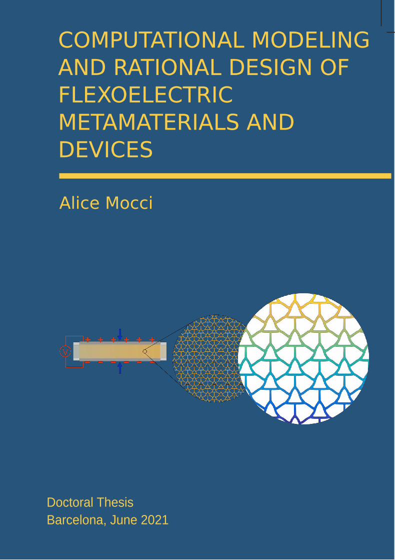
Doctoral ThesisBarcelona, June 2021
Alice Mocci
COMPUTATIONAL MODELING AND RATIONAL DESIGN OF FLEXOELECTRIC METAMATERIALS AND DEVICES
Computational modeling and
rational design of flexoelectric metamaterials and devices
Alice Mocci
ADVERTIMENT La consulta d’aquesta tesi queda condicionada a l’acceptació de les següents condicions d'ús: La difusió d’aquesta tesi per mitjà del repositori institucional UPCommons (http://upcommons.upc.edu/tesis) i el repositori cooperatiu TDX ( h t t p : / / w w w . t d x . c a t / ) ha estat autoritzada pels titulars dels drets de propietat intel·lectual únicament per a usos privats emmarcats en activitats d’investigació i docència. No s’autoritza la seva reproducció amb finalitats de lucre ni la seva difusió i posada a disposició des d’un lloc aliè al servei UPCommons o TDX. No s’autoritza la presentació del seu contingut en una finestra o marc aliè a UPCommons (framing). Aquesta reserva de drets afecta tant al resum de presentació de la tesi com als seus continguts. En la utilització o cita de parts de la tesi és obligat indicar el nom de la persona autora. ADVERTENCIA La consulta de esta tesis queda condicionada a la aceptación de las siguientes condiciones de uso: La difusión de esta tesis por medio del repositorio institucional UPCommons (http://upcommons.upc.edu/tesis) y el repositorio cooperativo TDR (http://www.tdx.cat/?locale- attribute=es) ha sido autorizada por los titulares de los derechos de propiedad intelectual únicamente para usos privados enmarcados en actividades de investigación y docencia. No se autoriza su reproducción con finalidades de lucro ni su difusión y puesta a disposición desde un sitio ajeno al servicio UPCommons No se autoriza la presentación de su contenido en una ventana o marco ajeno a UPCommons (framing). Esta reserva de derechos afecta tanto al resumen de presentación de la tesis como a sus contenidos. En la utilización o cita de partes de la tesis es obligado indicar el nombre de la persona autora. WARNING On having consulted this thesis you’re accepting the following use conditions: Spreading this thesis by the institutional repository UPCommons (http://upcommons.upc.edu/tesis) and the cooperative repository TDX (http://www.tdx.cat/?locale- attribute=en) has been authorized by the titular of the intellectual property rights only for private uses placed in investigation and teaching activities. Reproduction with lucrative aims is not authorized neither its spreading nor availability from a site foreign to the UPCommons service. Introducing its content in a window or frame foreign to the UPCommons service is not authorized (framing). These rights affect to the presentation summary of the thesis as well as to its contents. In the using or citation of parts of the thesis it’s obliged to indicate the name of the author.
Doctoral ThesisAdvisor: Irene AriasBarcelona, June 2021
Alice Mocci
Doctoral degree in Civil EngineeringDepartment of Civil and Environmental EngineeringUniversitat Politècnica de Catalunya
COMPUTATIONAL MODELING AND RATIONAL DESIGN OF FLEXOELECTRIC METAMATERIALS AND DEVICES

iii
UNIVERSITAT POLITÈCNICA DE CATALUNYA
Abstract
Computational modeling and rational design of flexoelectric metamaterials and devices
by Alice Mocci
Piezoelectricity, the two-way coupling between electric polarization and strain is the basicmechanism behind most electromechanical transduction technologies. It is possible onlyin a limited number of materials, namely those exhibiting a non-centrosymmetric atomicor molecular structure. Flexoelectricity, the two-way coupling between strain gradient andpolarization, and conversely polarization gradient and strain, is a universal property of alldielectrics. For most materials the flexoelectric coupling is relatively weak, and thus requireslarge gradients, which are attainable at small scales. Flexoelectricity thus provides a route todesign alternative materials and devices for electromechanical transduction exploiting fieldgradients at small scales, by itself or as a complement to piezoelectricity. It also broadens theclass of materials that can be used in these applications, overcoming the limitations of piezo-electrics regarding biocompatibility, toxicity and operating temperature. The present thesisfocuses on exploring theoretically the engineering concepts for the rational design of piezo-electric metamaterials and devices exploiting the flexoelectric effect in general dielectrics,including non-piezoelectrics.
This work relies on the premise that the material polarity required for an effective piezo-electric response, can be imprinted in the metamaterial through material architecture atthe microscale, thus eliminating the need for a non-centrosymmetric atomic and molecu-lar structure of the base-material. This concept is explored in detail and demonstrated in thethesis through accurate self-consistent simulations, showing that significant effective piezo-electricity can be achieved in non-piezoelectrics by accumulating the flexoelectric responseof small features under bending or torsion. This thesis proposes low area-fraction bending-dominated piezoelectric 2D periodic lattice metamaterial designs. The effective piezoelectricresponse is quantified and the effect of lattice geometry, orientation, feature size and area-fraction is revealed. Through computational homogenization, the full effective piezoelectrictensor is characterized, and a simple shape optimization study is presented, showing signif-icant enhancements relative to the initial designs. Designs for flexoelectric devices combin-ing multiple materials are also proposed, analyzed and quantified. As a possible buildingblock for three-dimensional metamaterials, the flexoelectric response of bars under torsionis studied in detail, identifying the conditions under which such a response is possible. Fur-thermore, this study has allowed us to propose an experimental setup to quantify the elusiveshear flexoelectric coefficient, one of the three independent components in cubic flexoelectricsystems.


v
Acknowledgements
At first, I would like to express my sincere gratitude to my supervisor, Prof. Irene Ariasfor sharing her deep knowledge enthusiastically, for creating an enjoyable environment thatstimulates original thinking and initiatives, and for allowing me to work on such a chal-lenging project. I truly appreciate her humanity and politeness, and her being continuouslysupportive, and patient.
I also want to acknowledge Dr. Amir Abdollahi for his kindness, support, and preciousadvice during the first years of my research. I am grateful for all the enjoyable moments andto have had the opportunity to work with him.
I extend my gratitude to Prof. Sonia Fernández-Méndez and my closer colleagues David,Jordi, and Prakhar. I enjoyed debating with them and I truly appreciate their constant sup-port and help.
I want to thank all my friends, for their true friendship and all the great shared moments.A special thanks to Caterina, for being the most amazing officemate, for her unfailing goodhumor, the relaxing coffee breaks and the happy times. To Carmen, my favorite flatmate andSpanish teacher other than a true friend, for all the wonderful memories.
I finally owe my heartfelt thankfulness to Luca and my family for their unconditionallove, support, and encouragement throughout all these years.
I gratefully acknowledge the financial support of the European Research Council (Start-ing Grant 679451 to Prof. Irene Arias).

vii
Contents
Abstract iii
Acknowledgements v
1 Introduction 11.1 Motivation . . . . . . . . . . . . . . . . . . . . . . . . . . . . . . . . . . . . . . . 11.2 Flexoelectricity: state of the art . . . . . . . . . . . . . . . . . . . . . . . . . . . 4
1.2.1 Evidence of flexoelectricity in various materials . . . . . . . . . . . . . 51.2.2 Characterization of flexoelectricity . . . . . . . . . . . . . . . . . . . . . 71.2.3 Harnessing flexoelectricity as a functional property . . . . . . . . . . . 101.2.4 Coexistence and competition between flexoelectricity and piezoelec-
tricity . . . . . . . . . . . . . . . . . . . . . . . . . . . . . . . . . . . . . . 121.3 Objectives of the thesis . . . . . . . . . . . . . . . . . . . . . . . . . . . . . . . . 131.4 Chapter overview . . . . . . . . . . . . . . . . . . . . . . . . . . . . . . . . . . . 151.5 List of publications . . . . . . . . . . . . . . . . . . . . . . . . . . . . . . . . . . 15
1.5.1 Publications derived from this thesis . . . . . . . . . . . . . . . . . . . . 151.5.2 Other related publications . . . . . . . . . . . . . . . . . . . . . . . . . . 16
1.6 Patents . . . . . . . . . . . . . . . . . . . . . . . . . . . . . . . . . . . . . . . . . 161.7 Conference proceedings . . . . . . . . . . . . . . . . . . . . . . . . . . . . . . . 16
2 Continuum model and two computational approaches for flexoelectricity 192.1 Continuum model . . . . . . . . . . . . . . . . . . . . . . . . . . . . . . . . . . . 192.2 Variational models . . . . . . . . . . . . . . . . . . . . . . . . . . . . . . . . . . 20
2.2.1 Direct flexoelectric form . . . . . . . . . . . . . . . . . . . . . . . . . . . 202.2.2 Lifshitz-invariant flexoelectric form . . . . . . . . . . . . . . . . . . . . 23
2.3 Numerical methods . . . . . . . . . . . . . . . . . . . . . . . . . . . . . . . . . . 252.3.1 Immersed boundary hierarchical B-splines approach . . . . . . . . . . 26
Nitsche’s method . . . . . . . . . . . . . . . . . . . . . . . . . . . . . . . 26B-spline basis functions . . . . . . . . . . . . . . . . . . . . . . . . . . . 27Immersed boundary method . . . . . . . . . . . . . . . . . . . . . . . . 28
2.3.2 Meshfree approximation scheme . . . . . . . . . . . . . . . . . . . . . . 29
3 Flexoelectricity-based piezoelectric metamaterials and devices 313.1 Introduction . . . . . . . . . . . . . . . . . . . . . . . . . . . . . . . . . . . . . . 313.2 Flexural scalable flexoelectric transducers . . . . . . . . . . . . . . . . . . . . . 333.3 Geometrically polarized architected dielectrics with effective piezoelectricity 34
3.3.1 Theoretical model and setup . . . . . . . . . . . . . . . . . . . . . . . . 353.3.2 Bending-dominated non-centrosymmetric lattices . . . . . . . . . . . . 373.3.3 Anisotropy and area fraction . . . . . . . . . . . . . . . . . . . . . . . . 393.3.4 Effective piezoelectric performance . . . . . . . . . . . . . . . . . . . . 41
viii
3.3.5 Generalized-periodic boundary conditions, validation and convergence 42Generalized-periodic boundary conditions . . . . . . . . . . . . . . . . 42Validation . . . . . . . . . . . . . . . . . . . . . . . . . . . . . . . . . . . 44Convergence . . . . . . . . . . . . . . . . . . . . . . . . . . . . . . . . . 44
3.4 Concluding remarks . . . . . . . . . . . . . . . . . . . . . . . . . . . . . . . . . 45
4 Computational homogenization of flexoelectric metamaterials 474.1 Introduction . . . . . . . . . . . . . . . . . . . . . . . . . . . . . . . . . . . . . . 474.2 Energy equivalence . . . . . . . . . . . . . . . . . . . . . . . . . . . . . . . . . . 484.3 Effective material tensors in the homogenized piezoelectric medium . . . . . 51
4.3.1 Computational homogenization: numerical approach . . . . . . . . . . 524.4 Results and Discussions . . . . . . . . . . . . . . . . . . . . . . . . . . . . . . . 53
4.4.1 Surface representation and symmetries . . . . . . . . . . . . . . . . . . 534.4.2 Effect of the nominal material properties . . . . . . . . . . . . . . . . . 55
4.5 Concluding remark . . . . . . . . . . . . . . . . . . . . . . . . . . . . . . . . . . 59
5 On-going work 615.1 Optimization methods . . . . . . . . . . . . . . . . . . . . . . . . . . . . . . . . 61
5.1.1 Gradient-based methods . . . . . . . . . . . . . . . . . . . . . . . . . . . 615.1.2 Genetic, population-based methods . . . . . . . . . . . . . . . . . . . . 63
5.2 Shape optimization of Design D0 . . . . . . . . . . . . . . . . . . . . . . . . . . 645.2.1 Longitudinal operation mode . . . . . . . . . . . . . . . . . . . . . . . . 655.2.2 Effect of the nominal material properties on the geometrically polar-
ized lattice . . . . . . . . . . . . . . . . . . . . . . . . . . . . . . . . . . . 665.3 On-going work . . . . . . . . . . . . . . . . . . . . . . . . . . . . . . . . . . . . 69
5.3.1 Transverse and shear operation mode . . . . . . . . . . . . . . . . . . . 69
6 Towards 3D flexoelectric metamaterials and devices: flexoelectricity under torsion 716.1 Torsion of a conical shaft with general cross section . . . . . . . . . . . . . . . 726.2 Self consistent quantification of flexoelectric roads under torsion . . . . . . . . 736.3 Chasing the elusive shear flexoelectricity . . . . . . . . . . . . . . . . . . . . . 796.4 Concluding remarks . . . . . . . . . . . . . . . . . . . . . . . . . . . . . . . . . 84
7 Conclusions and future work 877.1 Future work . . . . . . . . . . . . . . . . . . . . . . . . . . . . . . . . . . . . . . 88
A Immersed boundary B-Spline framework 91A.1 Material tensors . . . . . . . . . . . . . . . . . . . . . . . . . . . . . . . . . . . . 91
Elasticity tensor C . . . . . . . . . . . . . . . . . . . . . . . . . . . . . . 91Strain gradient elasticity tensor h . . . . . . . . . . . . . . . . . . . . . . 91Dielectricity tensor k . . . . . . . . . . . . . . . . . . . . . . . . . . . . . 92Electric field gradient dielectricity b . . . . . . . . . . . . . . . . . . . . 92Flexoelectricity tensor µ . . . . . . . . . . . . . . . . . . . . . . . . . . . 92
A.1.1 Strain gradient elasticity and electric field gradient dielectricity: sensi-tivity analysis . . . . . . . . . . . . . . . . . . . . . . . . . . . . . . . . . 92Cantilever beam bending . . . . . . . . . . . . . . . . . . . . . . . . . . 92Bending-dominated lattice metamaterials . . . . . . . . . . . . . . . . . 93
ix
B Piezoelectric coefficients and boundary conditions derivation for the homogenizedRVE 95B.1 Piezoelectricity . . . . . . . . . . . . . . . . . . . . . . . . . . . . . . . . . . . . 95
B.1.1 Energy forms . . . . . . . . . . . . . . . . . . . . . . . . . . . . . . . . . 95Internal energy U (#, D), h-form . . . . . . . . . . . . . . . . . . . . . . 95Gibbs energy F (s, E), d-form . . . . . . . . . . . . . . . . . . . . . . . 96Electric enthalpy H (#, E), e-form . . . . . . . . . . . . . . . . . . . . . . 97Elastic Gibbs function G1 (s, D), g-form . . . . . . . . . . . . . . . . . . 97
B.1.2 Relationship between piezoelectric tensors . . . . . . . . . . . . . . . . 98B.2 Tensor surface representation . . . . . . . . . . . . . . . . . . . . . . . . . . . . 99
C Meshfree approximation method 101C.1 Material characterization . . . . . . . . . . . . . . . . . . . . . . . . . . . . . . . 101
Elasticity tensor C . . . . . . . . . . . . . . . . . . . . . . . . . . . . . . 101Dielectricity tensor k . . . . . . . . . . . . . . . . . . . . . . . . . . . . . 101Flexoelectricity tensor µ . . . . . . . . . . . . . . . . . . . . . . . . . . . 101Gradient operators Bu and Bf . . . . . . . . . . . . . . . . . . . . . . . 102Hessian operators Hu and Hf . . . . . . . . . . . . . . . . . . . . . . . . 102
C.2 Derivation of the elastic torsion problem in cylindrical coordinates . . . . . . 102C.3 Mesh and convergence . . . . . . . . . . . . . . . . . . . . . . . . . . . . . . . . 103
Bibliography 105

xi
List of Figures
1.1 Electromechanical systems, adapted from Dagdeviren et al.[1]. . . . . . . . . . 11.2 Comparison of the main distinctive features of piezoelectricity, electrostriction
and flexoelectricity. . . . . . . . . . . . . . . . . . . . . . . . . . . . . . . . . . . 31.3 Number of publications on flexoelectricity from 1974 to 2020. Data has been
obtained from https://www.scopus.com/. . . . . . . . . . . . . . . . . . . . . 41.4 Flexoelectric mechanism in liquid crystals (LCs). . . . . . . . . . . . . . . . . . 51.5 Flexoelectricity in cellular membranes. . . . . . . . . . . . . . . . . . . . . . . . 61.6 Flexoelectricity in stereocilia in inner hair cells. . . . . . . . . . . . . . . . . . . 61.7 Flexoelectricity in bones. . . . . . . . . . . . . . . . . . . . . . . . . . . . . . . . 71.8 Flexoelectricity in hard materials. . . . . . . . . . . . . . . . . . . . . . . . . . . 71.9 Quantification of transverse and longitudinal flexoelectricity . . . . . . . . . . 91.10 Deformation mode in truncated pyramid under compression. . . . . . . . . . 101.11 Piezoelectric vs flexoelectric high-frequency bending resonator [42]. . . . . . . 101.12 Polarization switching in ferroelectric thin films due to flexoelectricity [51]. . 111.13 Nonpiezoelectric 2D sheets with circular and triangular inclusions . . . . . . 111.14 Piezoelectric composites based on flexoelectricity. . . . . . . . . . . . . . . . . 121.15 Interplay between piezoelectricity and flexoelectricity. . . . . . . . . . . . . . . 131.16 A properly designed flexoelectric metamaterial behaves as a piezoelectric ma-
terial at the macroscale. An electrical output is generated when a homoge-neous deformation is applied, or conversely it deforms under a uniform elec-trical bias. . . . . . . . . . . . . . . . . . . . . . . . . . . . . . . . . . . . . . . . 14
3.1 Publications on lead-free piezoceramics, from https://www.scopus.com/. . . . 323.2 Sketch of a piezoelectric device. . . . . . . . . . . . . . . . . . . . . . . . . . . . 323.3 Scalable effect in thin structural elements under bending . . . . . . . . . . . . 333.4 Scalable flexoelectric device. . . . . . . . . . . . . . . . . . . . . . . . . . . . . . 343.5 Schematic depiction of a periodic metamaterial in sensor or actuation mode . 353.6 Illustration of the generalized-periodic boundary conditions on a unit cell of
the periodic metamaterial. . . . . . . . . . . . . . . . . . . . . . . . . . . . . . . 363.7 Electric potential and displacements in centrosymmetric and non-centrosymmetric
devices under an applied deformation (sensor mode) and electric field (actu-ator mode). . . . . . . . . . . . . . . . . . . . . . . . . . . . . . . . . . . . . . . . 37
3.8 Geometrical parameters of the unit cell. . . . . . . . . . . . . . . . . . . . . . . 373.9 Electric field and y�displacement plotted on the deformed configuration for
various material designs in sensor and actuator mode. . . . . . . . . . . . . . . 383.10 Anisotropy of the effective piezoelectric coefficient in sensor and actuator
mode for Designs A to D. . . . . . . . . . . . . . . . . . . . . . . . . . . . . . . 403.11 Systematic examination of effective piezoelectric response of the architected
dielectrics, considering the optimal orientation and varying area fraction. . . 41
xii
3.12 Representative volume element (RVE) or unit cell of lattice design D. . . . . . 433.13 Electric potential jump as a function of the number of vertically stacked unit
cells for lattice Design C in displacement sensor mode. . . . . . . . . . . . . . 443.14 Relative error of two quantities of interest as a function of the element mesh
size h. The inset shows three representative computational mesh details. Allsimulations in this work have been computed with mesh level M1. . . . . . . 45
4.1 Heterogeneous structure and its equivalent homogeneous medium. . . . . . . 474.2 Effective elasticity, dielectricity and piezoelectricity tensors for Design A and
their surface representation. . . . . . . . . . . . . . . . . . . . . . . . . . . . . . 534.3 Effective elasticity, dielectricity and piezoelectricity tensors for Design B and
their surface representation. . . . . . . . . . . . . . . . . . . . . . . . . . . . . . 544.4 Effective elasticity, dielectricity and piezoelectricity tensors for Design C and
their surface representation. . . . . . . . . . . . . . . . . . . . . . . . . . . . . . 554.5 Effective elasticity, dielectricity and piezoelectricity tensors for Design D and
their surface representation. . . . . . . . . . . . . . . . . . . . . . . . . . . . . . 564.6 Effective elasticity, dielectricity and piezoelectricity tensors for Design D’ and
their surface representation. . . . . . . . . . . . . . . . . . . . . . . . . . . . . . 564.7 Non-zero independent components for the dielectricity, elasticity and piezo-
electricity tensors as a function of the nominal Young’s modulus. . . . . . . . 584.8 Non-zero independent components for the dielectricity, elasticity and piezo-
electricity tensors as a function of the nominal Young’s modulus. . . . . . . . 59
5.1 Gradient-based algorithm for optimization. . . . . . . . . . . . . . . . . . . . . 625.2 At each step the trust region is identified in order to better approximate the ob-
jective function f (xk). The picture has been taken from https://optimization.mccormick.northwestern.edu/index.php/Trust-region_methods. . . . . . 63
5.3 Population-based algorithm for optimization and terminology. . . . . . . . . . 645.4 The geometrical configuration of the most performant lattice design D’ is de-
fined by 8 parameters. . . . . . . . . . . . . . . . . . . . . . . . . . . . . . . . . 655.5 Shape optimization process for design D’ in longitudinal sensor h22 and g22
operation mode. A slab of the dimension of L = 10 ⇥ 10µm have been ex-tracted from our 2D lattice, therefore the resulting optimal shapes are in thesame scale and have the same fixed thickness t = 160nm. . . . . . . . . . . . . 66
5.6 Shape optimization process for design D0 in longitudinal actuator d22 and e22
operation mode. A slab of the dimension of L = 10 ⇥ 10µm have been ex-tracted from our 2D lattice, therefore the resulting optimal shapes are in thesame scale and have the same fixed thickness t = 160nm. . . . . . . . . . . . . 67
5.7 Cubic flexoelectric tensor . . . . . . . . . . . . . . . . . . . . . . . . . . . . . . . 675.8 . . . . . . . . . . . . . . . . . . . . . . . . . . . . . . . . . . . . . . . . . . . . . 695.9 Shape optimization process for design D’ in transverse d122 and shear d121 op-
eration mode. A slab of the dimension of L = 10 ⇥ 10µm have been extractedfrom our 2D lattice, therefore the resulting optimal shapes are in the samescale and have the same fixed thickness t = 160nm. . . . . . . . . . . . . . . . 70
6.1 Prismatic shaft under an applied constant torque T. The Cartesian (Ox1x2x3)
and the cylindrical (Orqz) reference systems are also reported. . . . . . . . . . 72
xiii
6.2 Twisting of a bar under an applied torque T around the z-axis. The infinitesi-mal angle df is the angle of torsion between a pair of cross-sections with theinfinitesimal distance dz apart. Cylindrical (r, q, z) coordinate system is de-picted. . . . . . . . . . . . . . . . . . . . . . . . . . . . . . . . . . . . . . . . . . 74
6.3 Electric potential distribution in (a) circular cross-section and (b) square cross-section. Electric potential is not generated in these setups.For visualizationpurposes, deformations are amplified by a factor of 30. . . . . . . . . . . . . . 75
6.4 Cone geometrical parameters, R1, R2 and L. . . . . . . . . . . . . . . . . . . . . 756.5 Distribution of electric potential for (a) anisotropic flexoelectricity and (b)
isotropic flexoelectricity. A non-ferroelectric electric potential pattern is ob-served for the case of anisotropic flexoelectricity only. Isotropic elastic proper-ties and circular cross-section are considered to isolate flexoelectric anisotropyfrom other sources of material or geometrical anisotropy.For visualization pur-poses, deformations are amplified by a factor of 30. . . . . . . . . . . . . . . . 75
6.6 Vector plot of the electric displacement D = µr# � krf along a circle on thecross-section not located on the lateral surface of the cone. Both individualcontributions to D are shown, the first one is decomposed into the angularand radial components, (µr#)q = µr# � µr# · n and (µr#)r = µr# · n, nbeing the outward unit normal to the circular cross-section. . . . . . . . . . . . 76
6.7 Distribution of electric potential in a truncated cone under (g) compressionand (h) bending. The yellow arrows represent the polarization direction. Theapplied displacements are represented by the black arrows. For visualizationpurposes, deformations are amplified by a factor of 30. . . . . . . . . . . . . . 76
6.8 (a) Distribution of electric potential in three different simulations with flex-oelectric tensors rotated different angles q = 0, p/6 and p/4, respectively.(b) Maximum magnitude of electric potential as a function of the flexoelectricanisotropy parameter for different geometrical configurations. . . . . . . . . . 78
6.9 Maximum magnitude of electric potential on the surface as a function of thegeometrical parameters. . . . . . . . . . . . . . . . . . . . . . . . . . . . . . . . 79
6.10 Truncated cone having radius R1, R2, respectively and length L. A groundelectrode is placed on the clamped end of the shaft while a torque T is appliedon the free-end. . . . . . . . . . . . . . . . . . . . . . . . . . . . . . . . . . . . . 80
6.11 Distribution of the electric potential f in a half truncated cone where a con-stant torque is applied on the right-end while the displacement and electricpotential are fixed on the left end. . . . . . . . . . . . . . . . . . . . . . . . . . . 81
6.12 Longitudinal and radial polarization in a half truncated cone under torsion. . 826.13 a) Deviation between the simulation and analytical results as a function of the
longitudinal µl and transversal µt flexoelectric coefficients. (b) Cross-sectionsof the deviation plot where µl = 0 (right) and µt = 0 (left). . . . . . . . . . . . 84
7.1 Electric potential distribution in the 3D extruded scalable flexoelectric deviceunder bending. . . . . . . . . . . . . . . . . . . . . . . . . . . . . . . . . . . . . 89
xiv
A.1 Flexoelectric cantilever beam with thickness t = 160nm. (a) Sensor mode, aforce F is enforced at the free end of the cantilever beam, the electric potentialf, reported in the contour plot, is measured at the top surface. (b) Actuatormode, an electric potential V is applied on the top face, while the bottom sidehas been grounded. The deflection j is measured. . . . . . . . . . . . . . . . . 93
A.2 Sensitivity analysis for Design D, with t = 40nm and t = 400nm. . . . . . . . 94
B.1 Spherical reference system Orqf. . . . . . . . . . . . . . . . . . . . . . . . . . . 100
C.1 (a) The rotation of the structured mesh by an angle z = 20 degrees does not af-fect the generation of the patterns in the electric potential distribution. Yellowlines have been added to highlight the rotation of the mesh. (b) Convergencestudy of the numerical simulations. The electric potential distribution doesnot change upon mesh refinement. . . . . . . . . . . . . . . . . . . . . . . . . . 104
xv
List of Tables
1.1 Centrosymmetric and non-centrosymmetric point groups . . . . . . . . . . . . 4
3.1 Material parameters . . . . . . . . . . . . . . . . . . . . . . . . . . . . . . . . . 343.2 Material parameters . . . . . . . . . . . . . . . . . . . . . . . . . . . . . . . . . 36
4.1 Numerical boundary conditions used to determine the unknown concentra-tion tensors and their derivatives. . . . . . . . . . . . . . . . . . . . . . . . . . . 52
4.2 Effective tensors coefficients . . . . . . . . . . . . . . . . . . . . . . . . . . . . . 57
5.1 Lower and upper bounds for the 8 design variables selected as minimizers forthis problem. . . . . . . . . . . . . . . . . . . . . . . . . . . . . . . . . . . . . . . 65
5.2 Lower and upper bounds for the 7 design variables selected as minimizers forthis problem. . . . . . . . . . . . . . . . . . . . . . . . . . . . . . . . . . . . . . . 68
6.1 Barium Strontium Titanate (BST). Material parameters. . . . . . . . . . . . . . 746.2 f coefficients . . . . . . . . . . . . . . . . . . . . . . . . . . . . . . . . . . . . . . 83

A nonno Antonino,che oggi sarebbe fiero di me.
1
Chapter 1
Introduction
1.1 Motivation
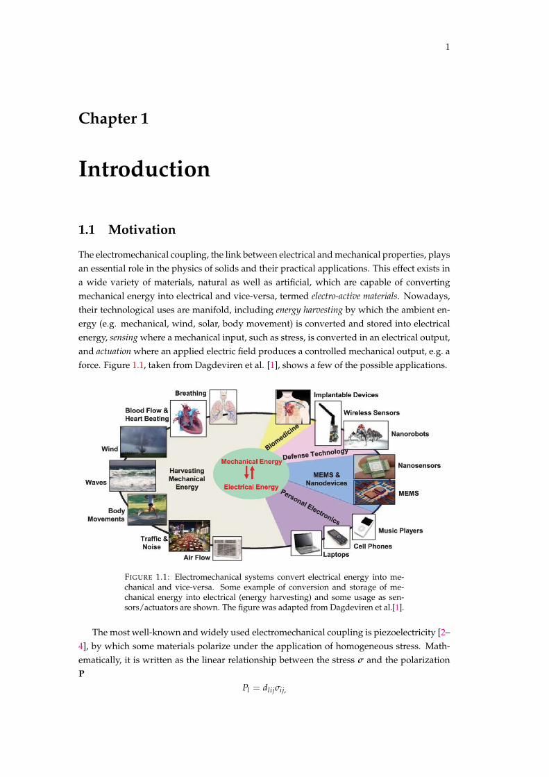
The electromechanical coupling, the link between electrical and mechanical properties, playsan essential role in the physics of solids and their practical applications. This effect exists ina wide variety of materials, natural as well as artificial, which are capable of convertingmechanical energy into electrical and vice-versa, termed electro-active materials. Nowadays,their technological uses are manifold, including energy harvesting by which the ambient en-ergy (e.g. mechanical, wind, solar, body movement) is converted and stored into electricalenergy, sensing where a mechanical input, such as stress, is converted in an electrical output,and actuation where an applied electric field produces a controlled mechanical output, e.g. aforce. Figure 1.1, taken from Dagdeviren et al. [1], shows a few of the possible applications.
FIGURE 1.1: Electromechanical systems convert electrical energy into me-chanical and vice-versa. Some example of conversion and storage of me-chanical energy into electrical (energy harvesting) and some usage as sen-sors/actuators are shown. The figure was adapted from Dagdeviren et al.[1].
The most well-known and widely used electromechanical coupling is piezoelectricity [2–4], by which some materials polarize under the application of homogeneous stress. Math-ematically, it is written as the linear relationship between the stress s and the polarizationP
Pl = dlijsij,
2 Chapter 1. Introduction
where d is the third-rank tensor of piezoelectricity [5]. The converse effect also exists,i.e. piezoelectric materials deform under an applied electrical field E,
#ij = dlijEl ,
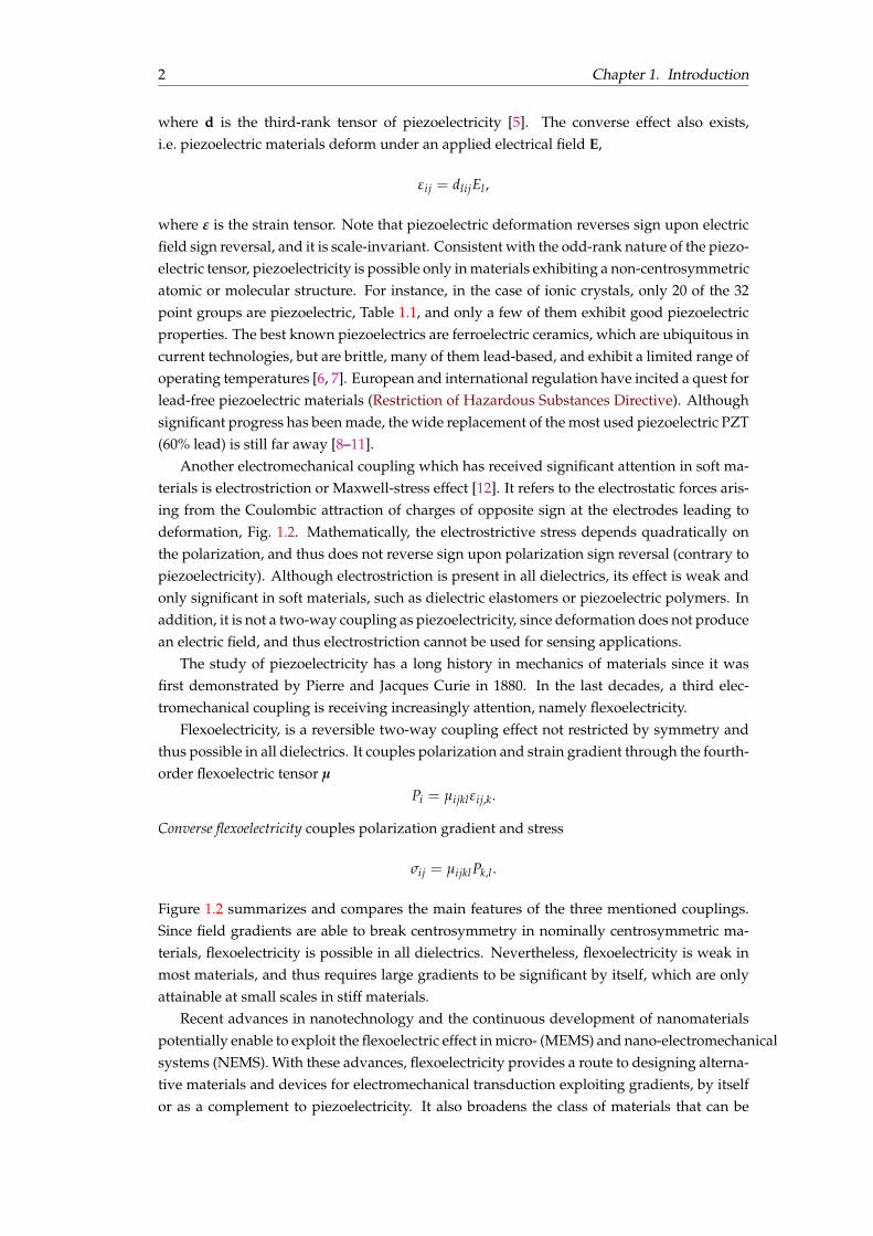
where # is the strain tensor. Note that piezoelectric deformation reverses sign upon electricfield sign reversal, and it is scale-invariant. Consistent with the odd-rank nature of the piezo-electric tensor, piezoelectricity is possible only in materials exhibiting a non-centrosymmetricatomic or molecular structure. For instance, in the case of ionic crystals, only 20 of the 32point groups are piezoelectric, Table 1.1, and only a few of them exhibit good piezoelectricproperties. The best known piezoelectrics are ferroelectric ceramics, which are ubiquitous incurrent technologies, but are brittle, many of them lead-based, and exhibit a limited range ofoperating temperatures [6, 7]. European and international regulation have incited a quest forlead-free piezoelectric materials (Restriction of Hazardous Substances Directive). Althoughsignificant progress has been made, the wide replacement of the most used piezoelectric PZT(60% lead) is still far away [8–11].
Another electromechanical coupling which has received significant attention in soft ma-terials is electrostriction or Maxwell-stress effect [12]. It refers to the electrostatic forces aris-ing from the Coulombic attraction of charges of opposite sign at the electrodes leading todeformation, Fig. 1.2. Mathematically, the electrostrictive stress depends quadratically onthe polarization, and thus does not reverse sign upon polarization sign reversal (contrary topiezoelectricity). Although electrostriction is present in all dielectrics, its effect is weak andonly significant in soft materials, such as dielectric elastomers or piezoelectric polymers. Inaddition, it is not a two-way coupling as piezoelectricity, since deformation does not producean electric field, and thus electrostriction cannot be used for sensing applications.
The study of piezoelectricity has a long history in mechanics of materials since it wasfirst demonstrated by Pierre and Jacques Curie in 1880. In the last decades, a third elec-tromechanical coupling is receiving increasingly attention, namely flexoelectricity.
Flexoelectricity, is a reversible two-way coupling effect not restricted by symmetry andthus possible in all dielectrics. It couples polarization and strain gradient through the fourth-order flexoelectric tensor µ
Pi = µijkl#ij,k.
Converse flexoelectricity couples polarization gradient and stress
sij = µijkl Pk,l .
Figure 1.2 summarizes and compares the main features of the three mentioned couplings.Since field gradients are able to break centrosymmetry in nominally centrosymmetric ma-terials, flexoelectricity is possible in all dielectrics. Nevertheless, flexoelectricity is weak inmost materials, and thus requires large gradients to be significant by itself, which are onlyattainable at small scales in stiff materials.
Recent advances in nanotechnology and the continuous development of nanomaterialspotentially enable to exploit the flexoelectric effect in micro- (MEMS) and nano-electromechanicalsystems (NEMS). With these advances, flexoelectricity provides a route to designing alterna-tive materials and devices for electromechanical transduction exploiting gradients, by itselfor as a complement to piezoelectricity. It also broadens the class of materials that can be
1.1. Motivation 3
+ +
++
-
+ +
++
-
V
F
F
+V
-V V
L/2
V
L
Electrostriction
Universality Scale invarianceTwo-way coupling Reversibility
+ +
++
-
F
V
V
F
+V
-V V
L/2
V
L
Piezoelectricity
Universality Scale invarianceTwo-way coupling Reversibility
F
V
V
F
+ +
++
-
+ +
++
-
+V
-V
V
L
2V
L/2
Flexoelectricity
Universality Scale invarianceTwo-way coupling Reversibility
Force FVibration Wave Voltage V
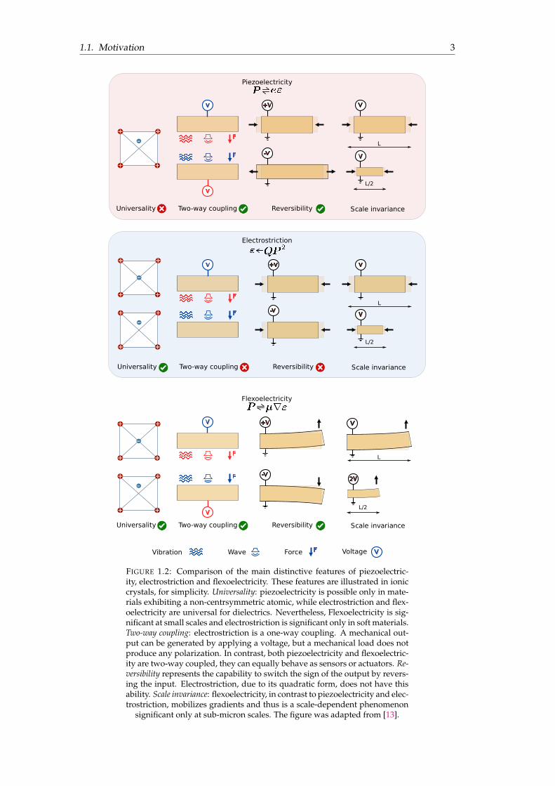
FIGURE 1.2: Comparison of the main distinctive features of piezoelectric-ity, electrostriction and flexoelectricity. These features are illustrated in ioniccrystals, for simplicity. Universality: piezoelectricity is possible only in mate-rials exhibiting a non-centrsymmetric atomic, while electrostriction and flex-oelectricity are universal for dielectrics. Nevertheless, Flexoelectricity is sig-nificant at small scales and electrostriction is significant only in soft materials.Two-way coupling: electrostriction is a one-way coupling. A mechanical out-put can be generated by applying a voltage, but a mechanical load does notproduce any polarization. In contrast, both piezoelectricity and flexoelectric-ity are two-way coupled, they can equally behave as sensors or actuators. Re-versibility represents the capability to switch the sign of the output by revers-ing the input. Electrostriction, due to its quadratic form, does not have thisability. Scale invariance: flexoelectricity, in contrast to piezoelectricity and elec-trostriction, mobilizes gradients and thus is a scale-dependent phenomenon
significant only at sub-micron scales. The figure was adapted from [13].
4 Chapter 1. Introduction
used in these applications, overcoming the limitations of piezoelectrics regarding biocom-patibility, toxicity and operating temperature. Hence, by exploiting field gradients at smallscale features, one can envision metamaterials and devices that effectively behave as piezo-electrics at the macroscale but are built from non-piezoelectric materials specifically chosento meet other application requirements.
TABLE 1.1: Centrosymmetric and non-centrosymmetric point groups
Point groupsCentrosymmetric Non-centrosymmetric (piezoelectric) Crystal system1 1 Triclinic2/m 2, m Monoclinicmmm 222,mm2 Orthorombic4/m,4/mmm 4,4,422,4mm,42m Tetragonal3,3m 3,32,3m Trigonal6/m,6/mmm 6,6,622,6mm,6m2 Hexagonalm3,m3m 23,43m,432 Cubic
1.2 Flexoelectricity: state of the art
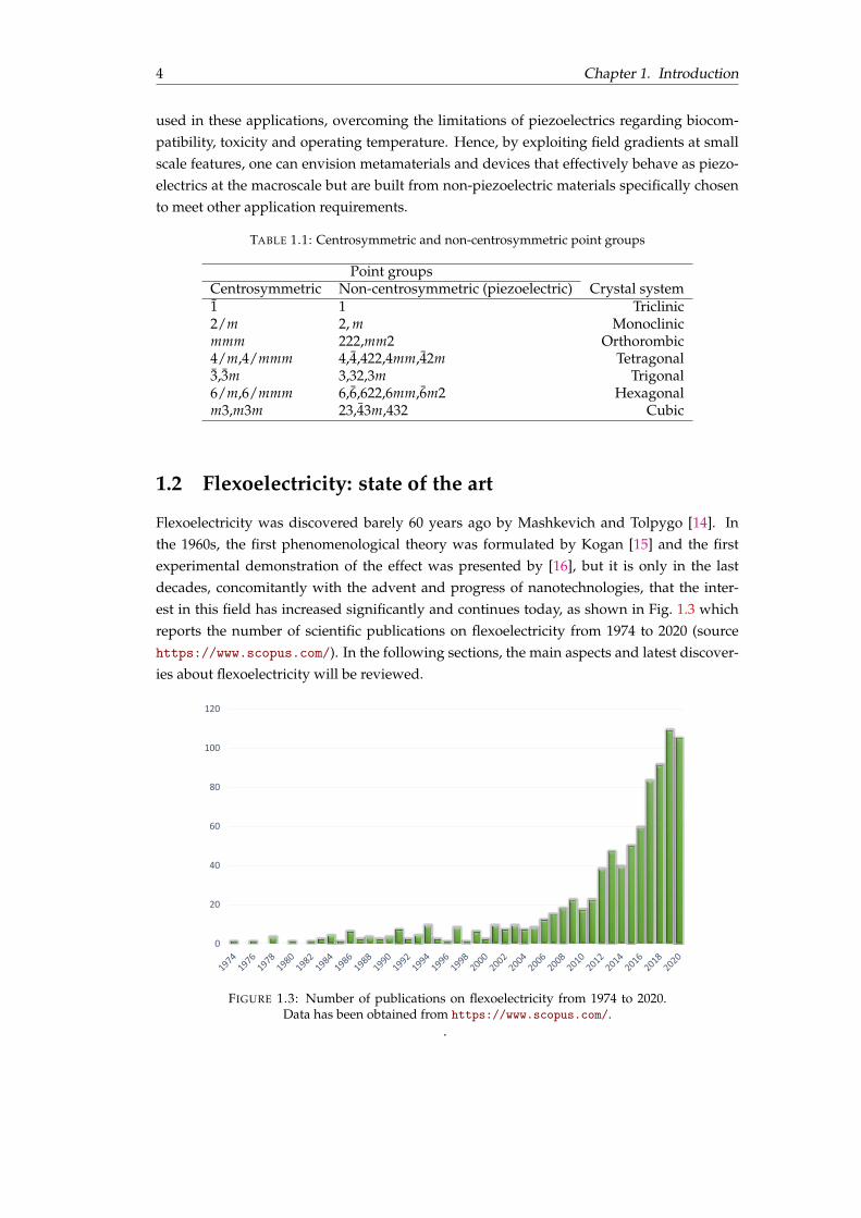
Flexoelectricity was discovered barely 60 years ago by Mashkevich and Tolpygo [14]. Inthe 1960s, the first phenomenological theory was formulated by Kogan [15] and the firstexperimental demonstration of the effect was presented by [16], but it is only in the lastdecades, concomitantly with the advent and progress of nanotechnologies, that the inter-est in this field has increased significantly and continues today, as shown in Fig. 1.3 whichreports the number of scientific publications on flexoelectricity from 1974 to 2020 (sourcehttps://www.scopus.com/). In the following sections, the main aspects and latest discover-ies about flexoelectricity will be reviewed.
0
20
40
60
80
100
120
FIGURE 1.3: Number of publications on flexoelectricity from 1974 to 2020.Data has been obtained from https://www.scopus.com/.
.
1.2. Flexoelectricity: state of the art 5
1.2.1 Evidence of flexoelectricity in various materials
The very first evidence of flexoelectricity dates back to 1968 when Bursian [16] performeda series of tests on Barium Titanate BaTiO3 thin films. In these experiments the crystalswere treated as actuators, namely, an electric field was applied in the transversal direction,leading to inhomogeneous deformation (bending) in the samples. Since then, flexoelectricityhas been observed in a wide variety of materials.
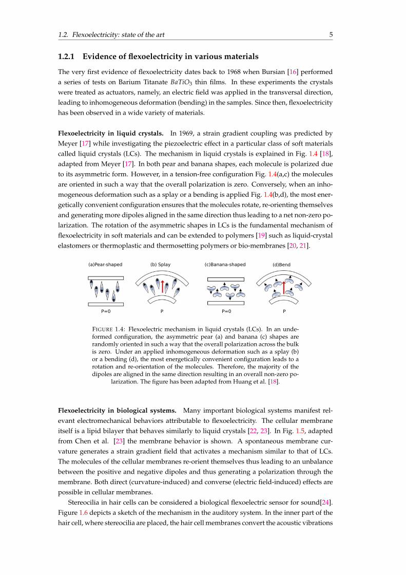
Flexoelectricity in liquid crystals. In 1969, a strain gradient coupling was predicted byMeyer [17] while investigating the piezoelectric effect in a particular class of soft materialscalled liquid crystals (LCs). The mechanism in liquid crystals is explained in Fig. 1.4 [18],adapted from Meyer [17]. In both pear and banana shapes, each molecule is polarized dueto its asymmetric form. However, in a tension-free configuration Fig. 1.4(a,c) the moleculesare oriented in such a way that the overall polarization is zero. Conversely, when an inho-mogeneous deformation such as a splay or a bending is applied Fig. 1.4(b,d), the most ener-getically convenient configuration ensures that the molecules rotate, re-orienting themselvesand generating more dipoles aligned in the same direction thus leading to a net non-zero po-larization. The rotation of the asymmetric shapes in LCs is the fundamental mechanism offlexoelectricity in soft materials and can be extended to polymers [19] such as liquid-crystalelastomers or thermoplastic and thermosetting polymers or bio-membranes [20, 21].
(a)Pear-shaped (b) Splay (c)Banana-shaped (d)Bend
P=0 P P=0 P
FIGURE 1.4: Flexoelectric mechanism in liquid crystals (LCs). In an unde-formed configuration, the asymmetric pear (a) and banana (c) shapes arerandomly oriented in such a way that the overall polarization across the bulkis zero. Under an applied inhomogeneous deformation such as a splay (b)or a bending (d), the most energetically convenient configuration leads to arotation and re-orientation of the molecules. Therefore, the majority of thedipoles are aligned in the same direction resulting in an overall non-zero po-
larization. The figure has been adapted from Huang et al. [18].
Flexoelectricity in biological systems. Many important biological systems manifest rel-evant electromechanical behaviors attributable to flexoelectricity. The cellular membraneitself is a lipid bilayer that behaves similarly to liquid crystals [22, 23]. In Fig. 1.5, adaptedfrom Chen et al. [23] the membrane behavior is shown. A spontaneous membrane cur-vature generates a strain gradient field that activates a mechanism similar to that of LCs.The molecules of the cellular membranes re-orient themselves thus leading to an unbalancebetween the positive and negative dipoles and thus generating a polarization through themembrane. Both direct (curvature-induced) and converse (electric field-induced) effects arepossible in cellular membranes.
Stereocilia in hair cells can be considered a biological flexoelectric sensor for sound[24].Figure 1.6 depicts a sketch of the mechanism in the auditory system. In the inner part of thehair cell, where stereocilia are placed, the hair cell membranes convert the acoustic vibrations
6 Chapter 1. Introduction
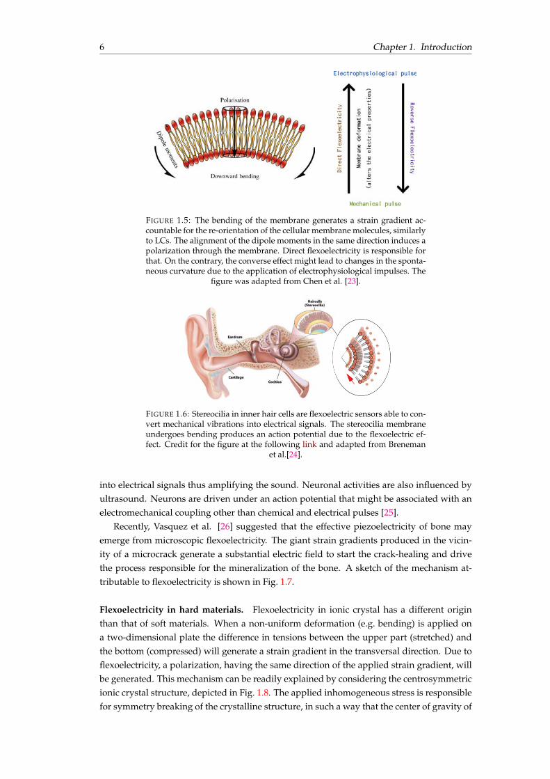
FIGURE 1.5: The bending of the membrane generates a strain gradient ac-countable for the re-orientation of the cellular membrane molecules, similarlyto LCs. The alignment of the dipole moments in the same direction induces apolarization through the membrane. Direct flexoelectricity is responsible forthat. On the contrary, the converse effect might lead to changes in the sponta-neous curvature due to the application of electrophysiological impulses. The
figure was adapted from Chen et al. [23].
FIGURE 1.6: Stereocilia in inner hair cells are flexoelectric sensors able to con-vert mechanical vibrations into electrical signals. The stereocilia membraneundergoes bending produces an action potential due to the flexoelectric ef-fect. Credit for the figure at the following link and adapted from Breneman
et al.[24].
into electrical signals thus amplifying the sound. Neuronal activities are also influenced byultrasound. Neurons are driven under an action potential that might be associated with anelectromechanical coupling other than chemical and electrical pulses [25].
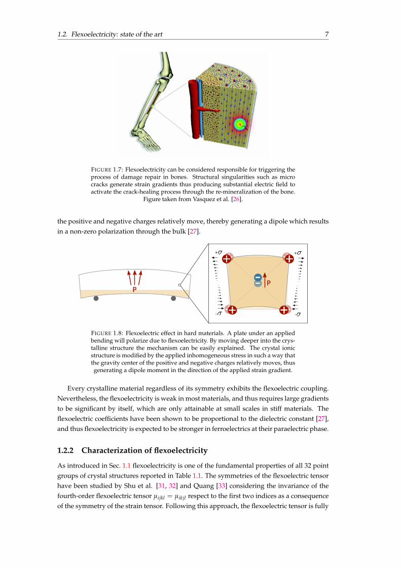
Recently, Vasquez et al. [26] suggested that the effective piezoelectricity of bone mayemerge from microscopic flexoelectricity. The giant strain gradients produced in the vicin-ity of a microcrack generate a substantial electric field to start the crack-healing and drivethe process responsible for the mineralization of the bone. A sketch of the mechanism at-tributable to flexoelectricity is shown in Fig. 1.7.
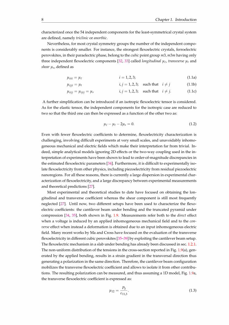
Flexoelectricity in hard materials. Flexoelectricity in ionic crystal has a different originthan that of soft materials. When a non-uniform deformation (e.g. bending) is applied ona two-dimensional plate the difference in tensions between the upper part (stretched) andthe bottom (compressed) will generate a strain gradient in the transversal direction. Due toflexoelectricity, a polarization, having the same direction of the applied strain gradient, willbe generated. This mechanism can be readily explained by considering the centrosymmetricionic crystal structure, depicted in Fig. 1.8. The applied inhomogeneous stress is responsiblefor symmetry breaking of the crystalline structure, in such a way that the center of gravity of
1.2. Flexoelectricity: state of the art 7
FIGURE 1.7: Flexoelectricity can be considered responsible for triggering theprocess of damage repair in bones. Structural singularities such as microcracks generate strain gradients thus producing substantial electric field toactivate the crack-healing process through the re-mineralization of the bone.
Figure taken from Vasquez et al. [26].
the positive and negative charges relatively move, thereby generating a dipole which resultsin a non-zero polarization through the bulk [27].
P
+
-
+
-
+ +
++
-
++
+ +- P
FIGURE 1.8: Flexoelectric effect in hard materials. A plate under an appliedbending will polarize due to flexoelectricity. By moving deeper into the crys-talline structure the mechanism can be easily explained. The crystal ionicstructure is modified by the applied inhomogeneous stress in such a way thatthe gravity center of the positive and negative charges relatively moves, thusgenerating a dipole moment in the direction of the applied strain gradient.
Every crystalline material regardless of its symmetry exhibits the flexoelectric coupling.Nevertheless, the flexoelectricity is weak in most materials, and thus requires large gradientsto be significant by itself, which are only attainable at small scales in stiff materials. Theflexoelectric coefficients have been shown to be proportional to the dielectric constant [27],and thus flexoelectricity is expected to be stronger in ferroelectrics at their paraelectric phase.
1.2.2 Characterization of flexoelectricity
As introduced in Sec. 1.1 flexoelectricity is one of the fundamental properties of all 32 pointgroups of crystal structures reported in Table 1.1. The symmetries of the flexoelectric tensorhave been studied by Shu et al. [31, 32] and Quang [33] considering the invariance of thefourth-order flexoelectric tensor µijkl = µikjl respect to the first two indices as a consequenceof the symmetry of the strain tensor. Following this approach, the flexoelectric tensor is fully
8 Chapter 1. Introduction
characterized once the 54 independent components for the least-symmetrical crystal systemare defined, namely triclinic or anorthic.
Nevertheless, for most crystal symmetry groups the number of the independent compo-nents is considerably smaller. For instance, the strongest flexoelectric crystals, ferroelectricperovskites, in their paraelectric phase, belong to the cubic point group m3, m3m having onlythree independent flexoelectric components [32, 33] called longitudinal µ`, transverse µt andshear µs, defined as
µiiii = µ` i = 1, 2, 3; (1.1a)
µijji = µt i, j = 1, 2, 3; such that i 6= j (1.1b)
µiijj = µijij = µs i, j = 1, 2, 3; such that i 6= j. (1.1c)
A further simplification can be introduced if an isotropic flexoelectric tensor is considered.As for the elastic tensor, the independent components for the isotropic case are reduced totwo so that the third one can then be expressed as a function of the other two as:
µ` � µt � 2µs = 0. (1.2)
Even with fewer flexoelectric coefficients to determine, flexoelectricity characterization ischallenging, involving difficult experiments at very small scales, and unavoidably inhomo-geneous mechanical and electric fields which make their interpretation far from trivial. In-deed, simple analytical models ignoring 2D effects or the two-way coupling used in the in-terpretation of experiments have been shown to lead to order-of-magnitude discrepancies inthe estimated flexoelectric parameters [34]. Furthermore, it is difficult to experimentally iso-late flexoelectricity from other physics, including piezoelectricity from residual piezoelectricnanoregions. For all these reasons, there is currently a large dispersion in experimental char-acterization of flexoelectricity, and a large discrepancy between experimental measurementsand theoretical predictions [27].
Most experimental and theoretical studies to date have focused on obtaining the lon-gitudinal and transverse coefficient whereas the shear component is still most frequentlyneglected [27]. Until now, two different setups have been used to characterize the flexo-electric coefficients: the cantilever beam under bending and the truncated pyramid undercompression [34, 35], both shown in Fig. 1.9. Measurements refer both to the direct effectwhen a voltage is induced by an applied inhomogeneous mechanical field and to the con-verse effect when instead a deformation is obtained due to an input inhomogeneous electricfield. Many recent works by Ma and Cross have focused on the evaluation of the transverseflexoelectricity in different cubic perovskites [35–39] by exploiting the cantilever beam setup.The flexoelectric mechanism in a slab under bending has already been discussed in sec. 1.2.1.The non-uniform distribution of the tensions in the cross-section reported in Fig. 1.9(a), gen-erated by the applied bending, results in a strain gradient in the transversal direction thusgenerating a polarization in the same direction. Therefore, the cantilever beam configurationmobilizes the transverse flexoelectric coefficient and allows to isolate it from other contribu-tions. The resulting polarization can be measured, and thus assuming a 1D model, Fig. 1.9a,the transverse flexoelectric coefficient is expressed as:
µ12 =P3
#11,3. (1.3)
1.2. Flexoelectricity: state of the art 9
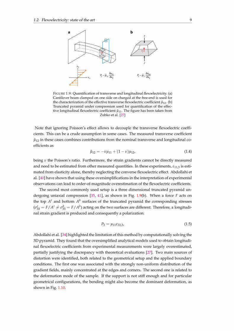
FIGURE 1.9: Quantification of transverse and longitudinal flexoelectricity. (a)Cantilever beam clamped on one side on charged at the free-end is used forthe characterization of the effective transverse flexoelectric coefficient µ12. (b)Truncated pyramid under compression used for quantification of the effec-tive longitudinal flexoelectric coefficient µ11. The figure has been taken from
Zubko et al. [27]
Note that ignoring Poisson’s effect allows to decouple the transverse flexoelectric coeffi-cients. This can be a crude assumption in some cases. The measured transverse coefficientµ12 in these cases combines contributions from the nominal transverse and longitudinal co-efficients as
µ12 = �nµ11 + (1 � n)µ12, (1.4)
being n the Poisson’s ratio. Furthermore, the strain gradients cannot be directly measuredand need to be estimated from other measured quantities. In these experiments, #11,3 is esti-mated from elasticity alone, thereby neglecting the converse flexoelectric effect. Abdollahi etal. [40] have shown that using these oversimplifications in the interpretation of experimentalobservations can lead to order-of-magnitude overestimation of the flexoelectric coefficients.
The second most commonly used setup is a three dimensional truncated pyramid un-dergoing uniaxial compression [35, 41], as shown in Fig. 1.9(b). When a force F acts onthe top At and bottom Ab surfaces of the truncated pyramid the corresponding stresses(st
33 = F/At 6= sb33 = F/Ab) acting on the two surfaces are different. Therefore, a longitudi-
nal strain gradient is produced and consequently a polarization:
P3 = µ11#33,3, (1.5)
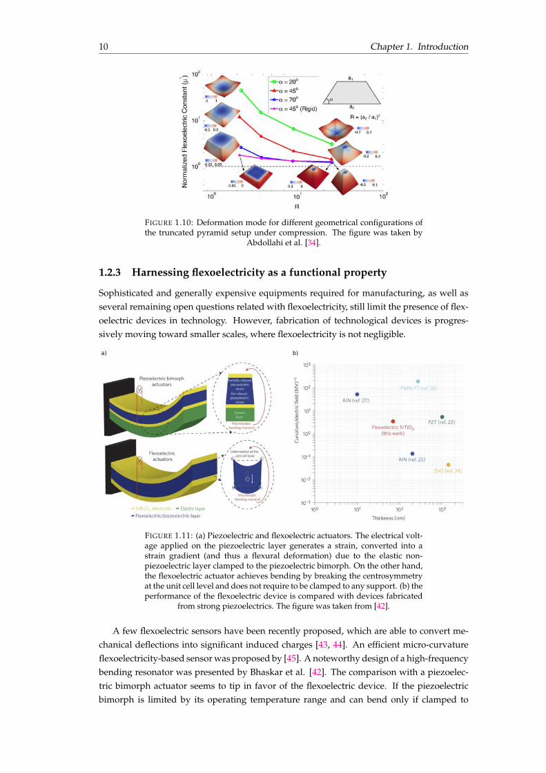
Abdollahi et al. [34] highlighted the limitation of this method by computationally solving the3D pyramid. They found that the oversimplified analytical models used to obtain longitudi-nal flexoelectric coefficients from experimental measurements were largely overestimated,partially justifying the discrepancy with theoretical evaluations [27]. Two main sources ofdistortion were identified, both related to the geometrical setup and the applied boundaryconditions. The first one was associated with the strongly non-uniform distribution of thegradient fields, mainly concentrated at the edges and corners. The second one is related tothe deformation mode of the sample. If the support is not stiff enough and for particulargeometrical configurations, the bending might also become the dominant deformation, asshown in Fig. 1.10.
10 Chapter 1. Introduction
FIGURE 1.10: Deformation mode for different geometrical configurations ofthe truncated pyramid setup under compression. The figure was taken by
Abdollahi et al. [34].
1.2.3 Harnessing flexoelectricity as a functional property
Sophisticated and generally expensive equipments required for manufacturing, as well asseveral remaining open questions related with flexoelectricity, still limit the presence of flex-oelectric devices in technology. However, fabrication of technological devices is progres-sively moving toward smaller scales, where flexoelectricity is not negligible.
a) b)
FIGURE 1.11: (a) Piezoelectric and flexoelectric actuators. The electrical volt-age applied on the piezoelectric layer generates a strain, converted into astrain gradient (and thus a flexural deformation) due to the elastic non-piezoelectric layer clamped to the piezoelectric bimorph. On the other hand,the flexoelectric actuator achieves bending by breaking the centrosymmetryat the unit cell level and does not require to be clamped to any support. (b) theperformance of the flexoelectric device is compared with devices fabricated
from strong piezoelectrics. The figure was taken from [42].
A few flexoelectric sensors have been recently proposed, which are able to convert me-chanical deflections into significant induced charges [43, 44]. An efficient micro-curvatureflexoelectricity-based sensor was proposed by [45]. A noteworthy design of a high-frequencybending resonator was presented by Bhaskar et al. [42]. The comparison with a piezoelec-tric bimorph actuator seems to tip in favor of the flexoelectric device. If the piezoelectricbimorph is limited by its operating temperature range and can bend only if clamped to
1.2. Flexoelectricity: state of the art 11
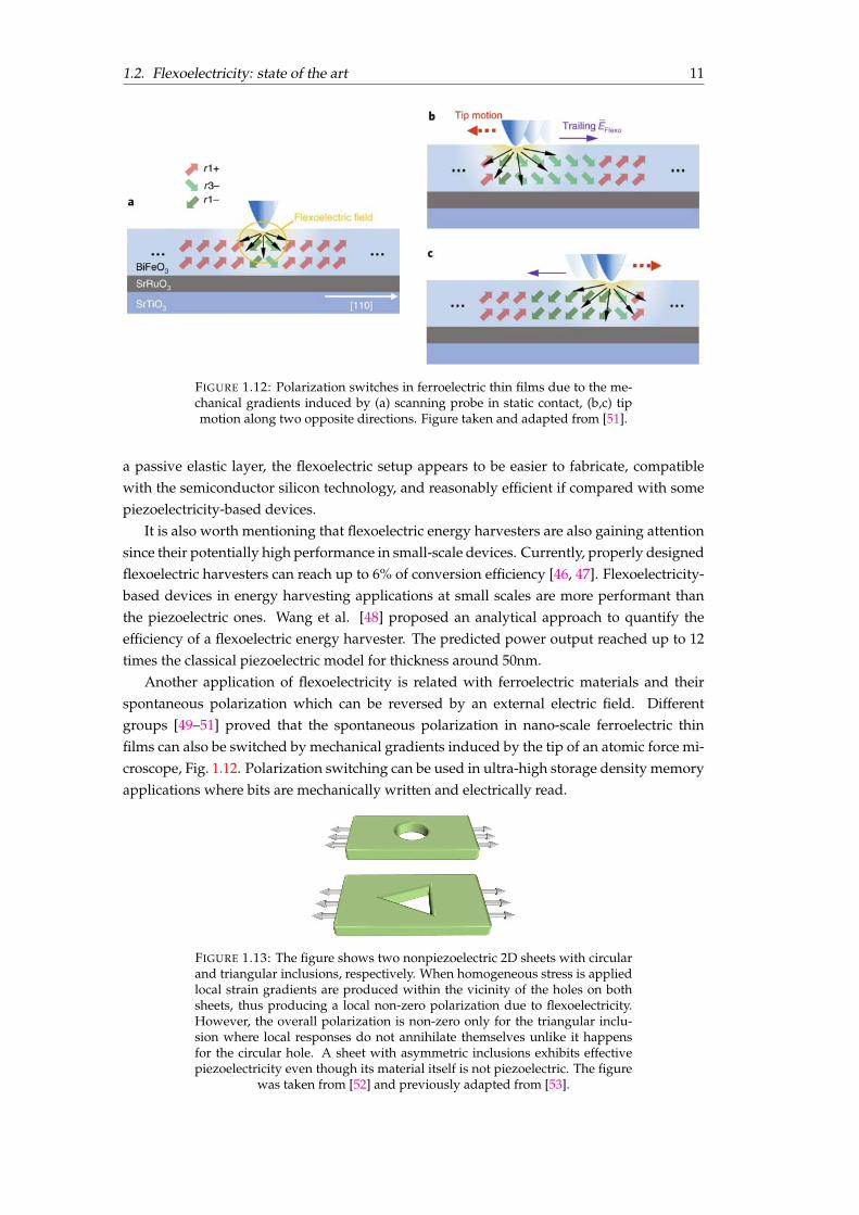
FIGURE 1.12: Polarization switches in ferroelectric thin films due to the me-chanical gradients induced by (a) scanning probe in static contact, (b,c) tipmotion along two opposite directions. Figure taken and adapted from [51].
a passive elastic layer, the flexoelectric setup appears to be easier to fabricate, compatiblewith the semiconductor silicon technology, and reasonably efficient if compared with somepiezoelectricity-based devices.
It is also worth mentioning that flexoelectric energy harvesters are also gaining attentionsince their potentially high performance in small-scale devices. Currently, properly designedflexoelectric harvesters can reach up to 6% of conversion efficiency [46, 47]. Flexoelectricity-based devices in energy harvesting applications at small scales are more performant thanthe piezoelectric ones. Wang et al. [48] proposed an analytical approach to quantify theefficiency of a flexoelectric energy harvester. The predicted power output reached up to 12times the classical piezoelectric model for thickness around 50nm.
Another application of flexoelectricity is related with ferroelectric materials and theirspontaneous polarization which can be reversed by an external electric field. Differentgroups [49–51] proved that the spontaneous polarization in nano-scale ferroelectric thinfilms can also be switched by mechanical gradients induced by the tip of an atomic force mi-croscope, Fig. 1.12. Polarization switching can be used in ultra-high storage density memoryapplications where bits are mechanically written and electrically read.
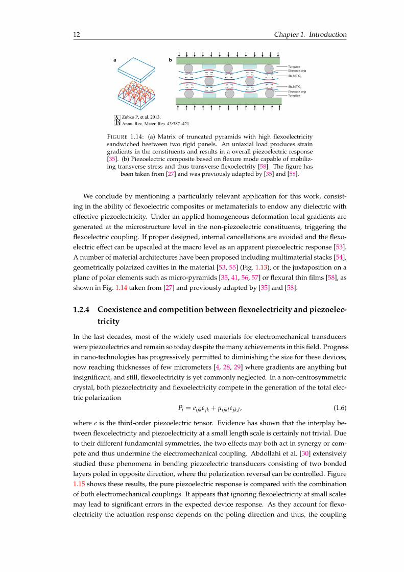
FIGURE 1.13: The figure shows two nonpiezoelectric 2D sheets with circularand triangular inclusions, respectively. When homogeneous stress is appliedlocal strain gradients are produced within the vicinity of the holes on bothsheets, thus producing a local non-zero polarization due to flexoelectricity.However, the overall polarization is non-zero only for the triangular inclu-sion where local responses do not annihilate themselves unlike it happensfor the circular hole. A sheet with asymmetric inclusions exhibits effectivepiezoelectricity even though its material itself is not piezoelectric. The figure
was taken from [52] and previously adapted from [53].
12 Chapter 1. Introduction
FIGURE 1.14: (a) Matrix of truncated pyramids with high flexoelectricitysandwiched beetween two rigid panels. An uniaxial load produces straingradients in the constituents and results in a overall piezoelectric response[35]. (b) Piezoelectric composite based on flexure mode capable of mobiliz-ing transverse stress and thus transverse flexoelectrity [58]. The figure has
been taken from [27] and was previously adapted by [35] and [58].
We conclude by mentioning a particularly relevant application for this work, consist-ing in the ability of flexoelectric composites or metamaterials to endow any dielectric witheffective piezoelectricity. Under an applied homogeneous deformation local gradients aregenerated at the microstructure level in the non-piezoelectric constituents, triggering theflexoelectric coupling. If proper designed, internal cancellations are avoided and the flexo-electric effect can be upscaled at the macro level as an apparent piezoelectric response [53].A number of material architectures have been proposed including multimaterial stacks [54],geometrically polarized cavities in the material [53, 55] (Fig. 1.13), or the juxtaposition on aplane of polar elements such as micro-pyramids [35, 41, 56, 57] or flexural thin films [58], asshown in Fig. 1.14 taken from [27] and previously adapted by [35] and [58].
1.2.4 Coexistence and competition between flexoelectricity and piezoelec-tricity
In the last decades, most of the widely used materials for electromechanical transducerswere piezoelectrics and remain so today despite the many achievements in this field. Progressin nano-technologies has progressively permitted to diminishing the size for these devices,now reaching thicknesses of few micrometers [4, 28, 29] where gradients are anything butinsignificant, and still, flexoelectricity is yet commonly neglected. In a non-centrosymmetriccrystal, both piezoelectricity and flexoelectricity compete in the generation of the total elec-tric polarization
Pi = eijk# jk + µijkl# jk,l , (1.6)
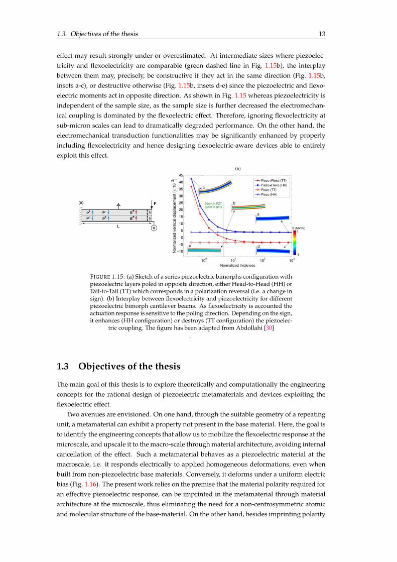
where e is the third-order piezoelectric tensor. Evidence has shown that the interplay be-tween flexoelectricity and piezoelectricity at a small length scale is certainly not trivial. Dueto their different fundamental symmetries, the two effects may both act in synergy or com-pete and thus undermine the electromechanical coupling. Abdollahi et al. [30] extensivelystudied these phenomena in bending piezoelectric transducers consisting of two bondedlayers poled in opposite direction, where the polarization reversal can be controlled. Figure1.15 shows these results, the pure piezoelectric response is compared with the combinationof both electromechanical couplings. It appears that ignoring flexoelectricity at small scalesmay lead to significant errors in the expected device response. As they account for flexo-electricity the actuation response depends on the poling direction and thus, the coupling
1.3. Objectives of the thesis 13
effect may result strongly under or overestimated. At intermediate sizes where piezoelec-tricity and flexoelectricity are comparable (green dashed line in Fig. 1.15b), the interplaybetween them may, precisely, be constructive if they act in the same direction (Fig. 1.15b,insets a-c), or destructive otherwise (Fig. 1.15b, insets d-e) since the piezoelectric and flexo-electric moments act in opposite direction. As shown in Fig. 1.15 whereas piezoelectricity isindependent of the sample size, as the sample size is further decreased the electromechan-ical coupling is dominated by the flexoelectric effect. Therefore, ignoring flexoelectricity atsub-micron scales can lead to dramatically degraded performance. On the other hand, theelectromechanical transduction functionalities may be significantly enhanced by properlyincluding flexoelectricity and hence designing flexoelectric-aware devices able to entirelyexploit this effect.
(b)
FIGURE 1.15: (a) Sketch of a series piezoelectric bimorphs configuration withpiezoelectric layers poled in opposite direction, either Head-to-Head (HH) orTail-to-Tail (TT) which corresponds in a polarization reversal (i.e. a change insign). (b) Interplay between flexoelectricity and piezoelectricity for differentpiezoelectric bimorph cantilever beams. As flexoelectricity is accounted theactuation response is sensitive to the poling direction. Depending on the sign,it enhances (HH configuration) or destroys (TT configuration) the piezoelec-
tric coupling. The figure has been adapted from Abdollahi [30].
1.3 Objectives of the thesis
The main goal of this thesis is to explore theoretically and computationally the engineeringconcepts for the rational design of piezoelectric metamaterials and devices exploiting theflexoelectric effect.
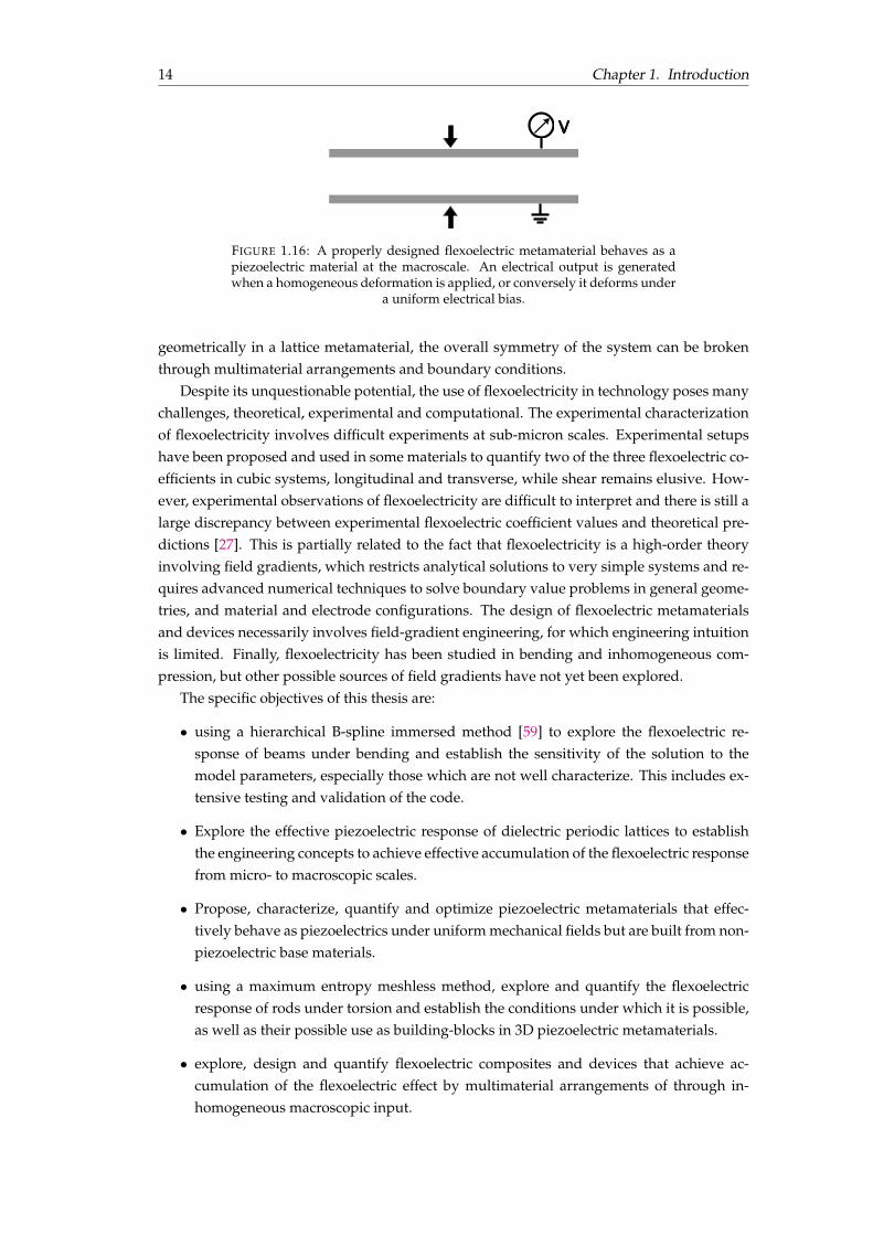
Two avenues are envisioned. On one hand, through the suitable geometry of a repeatingunit, a metamaterial can exhibit a property not present in the base material. Here, the goal isto identify the engineering concepts that allow us to mobilize the flexoelectric response at themicroscale, and upscale it to the macro-scale through material architecture, avoiding internalcancellation of the effect. Such a metamaterial behaves as a piezoelectric material at themacroscale, i.e. it responds electrically to applied homogeneous deformations, even whenbuilt from non-piezoelectric base materials. Conversely, it deforms under a uniform electricbias (Fig. 1.16). The present work relies on the premise that the material polarity required foran effective piezoelectric response, can be imprinted in the metamaterial through materialarchitecture at the microscale, thus eliminating the need for a non-centrosymmetric atomicand molecular structure of the base-material. On the other hand, besides imprinting polarity
14 Chapter 1. Introduction
V
FIGURE 1.16: A properly designed flexoelectric metamaterial behaves as apiezoelectric material at the macroscale. An electrical output is generatedwhen a homogeneous deformation is applied, or conversely it deforms under
a uniform electrical bias.
geometrically in a lattice metamaterial, the overall symmetry of the system can be brokenthrough multimaterial arrangements and boundary conditions.
Despite its unquestionable potential, the use of flexoelectricity in technology poses manychallenges, theoretical, experimental and computational. The experimental characterizationof flexoelectricity involves difficult experiments at sub-micron scales. Experimental setupshave been proposed and used in some materials to quantify two of the three flexoelectric co-efficients in cubic systems, longitudinal and transverse, while shear remains elusive. How-ever, experimental observations of flexoelectricity are difficult to interpret and there is still alarge discrepancy between experimental flexoelectric coefficient values and theoretical pre-dictions [27]. This is partially related to the fact that flexoelectricity is a high-order theoryinvolving field gradients, which restricts analytical solutions to very simple systems and re-quires advanced numerical techniques to solve boundary value problems in general geome-tries, and material and electrode configurations. The design of flexoelectric metamaterialsand devices necessarily involves field-gradient engineering, for which engineering intuitionis limited. Finally, flexoelectricity has been studied in bending and inhomogeneous com-pression, but other possible sources of field gradients have not yet been explored.
The specific objectives of this thesis are:
• using a hierarchical B-spline immersed method [59] to explore the flexoelectric re-sponse of beams under bending and establish the sensitivity of the solution to themodel parameters, especially those which are not well characterize. This includes ex-tensive testing and validation of the code.
• Explore the effective piezoelectric response of dielectric periodic lattices to establishthe engineering concepts to achieve effective accumulation of the flexoelectric responsefrom micro- to macroscopic scales.
• Propose, characterize, quantify and optimize piezoelectric metamaterials that effec-tively behave as piezoelectrics under uniform mechanical fields but are built from non-piezoelectric base materials.
• using a maximum entropy meshless method, explore and quantify the flexoelectricresponse of rods under torsion and establish the conditions under which it is possible,as well as their possible use as building-blocks in 3D piezoelectric metamaterials.
• explore, design and quantify flexoelectric composites and devices that achieve ac-cumulation of the flexoelectric effect by multimaterial arrangements of through in-homogeneous macroscopic input.
1.4. Chapter overview 15
1.4 Chapter overview
The manuscript is divided into two main parts, respectively regarding the identification oftwo-dimensional and three-dimensional suitable setups for constructively accumulating theflexoelectric effect in non-piezoelectric dielectrics. In Chapter 2 we summarize the theoreticaland numerical tools that have been used to perform the work object of this thesis. In Chapter3 we propose a new class of 2D flexoelectric-based metamaterials enabling piezoelectricityin non-piezoelectric dielectrics. Chapter 4 concerns a computational homogenization tech-nique to perform a comprehensive study of the proposed architected materials, whereas inChapter 5 we perform a shape optimization study of the aforementioned metamaterials. InChapter 6, we propose guidelines for understanding the torsion problem in 3D flexoelec-tric rods and we present a novel approach for the quantification of the shear flexoelectriccoefficient. Chapter 7 summarizes and concludes the manuscript.
1.5 List of publications
1.5.1 Publications derived from this thesis
• A.Mocci, J.Barceló-Mercader, D.Codony and I.Arias. Geometrically polarized architected di-electrics with effective piezoelectricity. (Submitted.) [60].
We propose a class of metamaterials with piezoelectric-like behavior, which can bemade out in principle of any dielectric material. To achieve significant piezoelectricity,we show that it is sufficient to suitably design the geometry of the material micro-architecture so that it contains thin elements subjected to bending and lacks mirrorsymmetry. We thus identify simple rules to turn a micro-architected metamaterial intoa piezoelectric. The reader can find correspondence in Ch. 3, sec. 3.3.
• A.Mocci, P.Gupta and I.Arias. Shape optimization of architected dielectrics with effectivepiezoelectricity using computational homogenization. (In preparation.) [61].
This paper develops a computational homogenization technique for flexoelectric-basedarchitected dielectrics lacking piezoelectricity. We compute and characterize the over-all behavior of micro-architected metamaterials proposed in [60]. We define the pre-ferred operation mode and propose a systematic shape optimization for each of theaforementioned lattices. The work reported in this publication is addressed in Ch. 4and Ch. 5 of this manuscript.
• A.Mocci, A.Abdollahi and I.Arias. Flexoelectricity in dielectrics under torsion. (Submitted.)[62].
In this paper, we show that mechanical torsion of conical rods generically induces po-larization domains and that these domains critically depend on flexoelectric anisotropyin materials with cubic symmetry. We further identify how the polarization domainsdepend on rod geometry and we establish conditions under which flexoelectricitymanifests itself during torsion of thin rods, a canonical method to generate strain gra-dients. This work is reported in Ch. 6, sec. 6.2.
• A.Mocci, A.Abdollahi and I.Arias. Flexoelectric bars under torsion: chasing the elusive shearflexoelectricity. (To be submitted.) [63].
16 Chapter 1. Introduction
Flexoelectricity (the coupling between strain gradient and polarization and converselystrain and polarization gradients) is particularly strong in ferroelectrics. However,there is not yet a universal agreement on the magnitude and even sign of the flex-oelectric coefficients in these materials. This situation is even more dramatic in thecase of the shear flexoelectric coefficient since generating a measurable polarizationinduced by shear strain gradient is nontrivial. Based on torsion mechanics and us-ing three-dimensional self-consistent simulations of flexoelectricity, we propose here anovel approach to quantify shear flexoelectricity in ferroelectrics. This approach alsoprovides a validation benchmark for computational models of flexoelectricity. Thereader is referred to Ch. 6, 6.3 for details about this work.
1.5.2 Other related publications
• D.Codony, A.Mocci, O.Marco and I.Arias. Wheel-shaped and helical torsional flexoelectricdevices. (In preparation.) [64].
With regards to the scalable flexoelectric device discussed in sec. 3.2, here we presenttorsional actuation able to induce bending in the internal component of a wheel-shapeddevice [13]. Extending this concept to three-dimensional scalable devices the flexoelec-tric effect is upscaled and a much larger net electric voltage is obtained.
• J.Barceló-Mercader, A.Mocci, D.Codony and I.Arias. Generalized periodicity conditions forcomputational modeling of flexoelectric metamaterials. (To be submitted.) [65].
In this paper, we develop a method to enforce generalized periodic conditions. Thanksto this method the computational domain of an architected materials with periodicmicrostructure can be reduced to a single unit cell and thus the bulk response is effi-ciently evaluated without the need of considering a sufficiently large part of the wholedomain.
1.6 Patents
• I.Arias, A.Abdollahi, A.Mocci and D.Codony. Lattice structure with piezoelectric behavior, aforce or movement sensor and an actuator containing said lattice structure. European patentoffice. (2020).
This patent, currently in PCT phase, contains the architected flexoelectric-based mate-rials proposed in Ch. 3.
1.7 Conference proceedings
During the Ph.D., the work object of this thesis has been presented in several national andinternational conferences.
• A.Mocci, A.Abdollahi and I.Arias. Quantification of shear flexoelectricity in ferroelectrics.16th European Mechanics of Materials Conference (EMMC16), Nantes, France (2018).
• A.Mocci, A.Abdollahi and I.Arias. Quantification of shear flexoelectricity in ferroelectrics.10th European Solid Mechanics Conference (ESMC2018), Bologna, Italy (2018).

1.7. Conference proceedings 17
• A.Mocci, D.Codony, A.Abdollahi and I.Arias. Flexoelectricity-based electromechanical meta-materials. Symposium on Architectured material mechanics (IUTAM2018AMS), Chicago,IL(USA) (2018).
• A.Mocci, A.Abdollahi and I.Arias. Flexoelectricity-based electromechanical metamaterials.55th Technical Meeting of the Society of Engineering Science (SES2018), Madrid, Spain(2018).

19
Chapter 2
Continuum model and twocomputational approaches forflexoelectricity
This chapter provides an overview of the two theoretical and computational frameworksthat have been used to analyze and quantify the electromechanical response of flexoelectricmetamaterials and devices. It is not intended to be exhaustive and the reader will be referredto the author’s contributions.
The details about the derivations have been partially extracted from Abdollahi et al.[40]and Dr.David Codony’s Ph. D dissertation [13] and recent publication [59].
2.1 Continuum model
Theoretical models of flexoelectricity are essential to fully understand and exploit this ef-fect. The first phenomenological model was proposed by Kogan in 1964 [15] and later ex-tended by Mindlin in 1968 [66]. However, we must leap almost twenty years before flex-oelectricity was seen as a separated electromechanical effect in crystalline dielectrics, dis-tinct from piezoelectricity. Only then, an exhaustive theoretical model was proposed [67,68]. Nowadays, there are different phenomenological models that describe the flexoelectricphenomenon (the reader is referred to recent reviews on flexoelectricity for an exhaustiveoverview on the subject [27, 69, 70]).
To define a non-piezoelectric dielectric material within the continuum framework, onecan write different models based on the choice of the state variables describing the flexoelec-tric effect. This results in different energy forms:
• Internal energy U (#,r#, D,rD),
• Gibbs function F(s,rs, E,rE),
• Electric enthalpy H(#,r#, E,rE),
• Elastic Gibbs function G1(s,rs, D,rD),
where D and E represent the electric displacement and electric field, respectively.

20 Chapter 2. Continuum model and two computational approaches for flexoelectricity
Among all the energy forms, the electric enthalpy H is often considered more convenientsince its dependence on the electric field instead of the electric displacement. The Maxwell-Faraday’s law (r⇥ E = 0), indeed presumes that an electric potential f exists such that
E = �rf.
Thus, by selecting the electric potential f as the electrical unknown the Maxwell-Faraday’slaw is automatically satisfied and does not require any extra constraint.
Several flexoelectric enthalpy forms can be written, mainly depending on the consideredflexoelectric coupling. In the next sections and chapters we will refer to two different en-thalpy forms, namely the Direct HhDiri and the Lifshitz-invariant HhLi f i form, which haveboth been used for this work.
2.2 Variational models
Although different enthalpy forms lead to the same Euler-Lagrange equations, differentboundary value problems must be derived since they give rise to different boundary condi-tion definitions.
Considering the generic free enthalpy form H , defined to mathematically describe theflexoelectric coupling, and W ext the work done by the external sources, the variational for-mulation associated to the problem is written as [40]
P[u, E] =Z
WH(u, E)dW �W ext. (2.1)
The following related variational principle corresponds to an unconstrained optimizationproblem
(u⇤, f⇤) = arg minu
maxf
P[u,�rf]. (2.2)
2.2.1 Direct flexoelectric form
The Direct enthalpy form HhDiri is written as
HhDiri(#,r#, E) :=12
#ijCijkl#kl +12
#ij,khijklmn# lm,n �12
ElklmEm � Elµlijk#ij,k, (2.3)
where the mechanical displacement field u and the electric potential f (s. t. , E = �rf),are the unknown independent variables. The pure mechanical terms are represented by theforth-order elasticity tensor C, with # = 1/2(ru +ruT) being the strain gradient tensor,h the sixth-order strain gradient elasticity tensor, whereas k is the second-order dielectricitytensor. The electromechanical coupling is represented by the fourth-order direct flexoelectrictensor µ. From a dimensional argument, h and C induce and elastic length-scale `mech, whileC, k, µ induce a flexoelectric length scale ` f lexo that controls the size-dependence of the effect.The reader can refer to the App. A and C for further details about the tensors [40] and theirimplementation.
2.2. Variational models 21
Having defined the physical domain W, its boundary ∂W and its edges C, the admissiblesources of external work are
WW(u, f) := �biui + qf, (2.4a)
W∂W(u, f) := �tiui � ri∂nui + wf (2.4b)
WC(u, f) := �jiui, (2.4c)
where b and q are body forces and free electric charges (i.e. forces per unit volume), t and rthe tractions and double tractions (i.e. force and moment per unit area), w the surface chargedensity (i.e. electric charge per unit area) and j the surface tension (i.e. force per unit length).
The boundary ∂W is split into ∂W = ∂Wu [ ∂Wt = ∂Wv [ ∂Wr = ∂Wf [ ∂Ww, being∂Wu, ∂Wv and ∂Wf the Dirichlet boundaries, where displacement field u, its normal deriva-tive v and electric potential f are prescribed, and ∂Wt, ∂Wr and ∂Ww the Neumann bound-aries, where values for traction t, double traction r and surface charge density w are applied.The edges C are also split into Dirichlet Cu and Neumann Cj edges, corresponding to pre-scribed displacement or surface tension j, respectively.
The corresponding boundary and edge conditions are written as:
u � u = 0 on ∂Wu, t(u, f)� t = 0 on ∂Wt, (2.5a)
∂n(u)� v = 0 on ∂Wv, r(u, f)� r = 0 on ∂Wr, (2.5b)
f � f = 0 on ∂Wf, w(u, f)� w = 0 on ∂Ww, (2.5c)
u � u = 0 on Cu, j(u, f)� j = 0 on Cj. (2.5d)
It is worth highlighting that despite finite elements or meshless frameworks, where bound-ary conditions on ∂Wu are enforced strongly, automatically fulfilling the edge conditions, ina context where boundary conditions are weakly imposed, neglecting the edge condition onCu would be analogous to erroneously considering homogeneous Neumann conditions onDirichlet edges.
Following the standard approach in computational mechanics, Dirichlet boundary con-ditions are not included explicitly into the weak form since they are already fulfilled by aproper choice of the functional spaces. An alternative Nitsche’s method for weak imposi-tion of the boundary conditions was recently derived, we refer to Codony et al.[59] for thefull derivation. The enthalpy functional in Eq. (2.1) is written as
PhDiriD [u, f] =
Z
W
⇣HhDiri(#(u),r#(u), E(f)� biui + qf
⌘dW
+Z
∂Wt�tiuidG +
Z
∂Wr�ri∂
nuidG +Z
∂Ww
wfdG +Z
Cj� jiuids. (2.6)
The equilibrium states (u⇤, f⇤) corresponds to the saddle point of the enthalpy potential,fulfilling the variational principle
(u⇤, f⇤) = arg minu2VD
maxf2PD
PhDiriD [u, f], (2.7)
22 Chapter 2. Continuum model and two computational approaches for flexoelectricity
with the functional space VD and PD having sufficient regularity and fulfilling the Dirichletboundary conditions in Eq. (2.5), that is:
VD := {u 2 [H2(W)]3 | u � u = 0 on ∂Wu and on Cu, and ∂nu � v = 0 on ∂Wv}, (2.8a)
PD := {f 2 H1(W) | f � f = 0 on ∂Wf}. (2.8b)
The weak form of the problem is found by enforcing dPhDiriD = 0 for all admissible variations
du 2 V0 and df 2 P0, with
V0 := {du 2 [H2(W)]3 | du = 0 on ∂Wu and on Cu, and ∂ndu = 0 on ∂Wv}, (2.9a)
P0 := {df 2 H1(W) | df = 0 on ∂Wf}. (2.9b)
The weak form reads: Find (u, f) 2 VD ⌦ PD such that, 8(du, df) 2 V0 ⌦ P0,
dPhDiriD ⌘ duPhDiri
D + dfPhDiriD
⌘Z
W(sijd#ij + sijkd#ij,k � DldEl � bidui + qdf)dW
+Z
∂Wt�tiduidG +
Z
∂Wr�ri∂
nduidG +Z
∂Ww
wdfdG +Z
Cj� jiduids = 0, (2.10)
having definedd# := #(du), dr# := r#(du), dE := E(df).
Integrating by parts and making use of the divergence and surface divergence theorems [59],the Euler-Lagrange equations are obtained
8<
:(sij � sijk,k), j + bi = 0 in W
Dl,l � q = 0 in W.(2.11)
The Cauchy stress s and the hyper stress s in Eqs. (2.10) and (2.11) represent the conjugatequantities to the strain # and the strain gradient r#, respectively, and can thus be derivedfrom the electromechanical enthalpy as
sij(#,r#, E) :=∂HhDiri
∂#ij= Cijkl#kl , (2.12a)
sijk(#,r#, E) :=∂HhDiri
∂#ij,k= hijklmn# lm,n � µlijkEl . (2.12b)
Hence, the physical stress, from Eqs. (2.11), is defined as
sij(#,r#, E) := sij(#,r#, E)� sijk(#,r#, E) = Cijkl#kl � hijklmn# lm,n + µlijkEl (2.13)
Similarly, the conjugate quantity to the electric field E is the electric displacement D inEqs. (2.10) and (2.11), therefore
Dl(#,r#, E) :=∂HhDiri
∂El= �klmEm � µlijk#ij,k. (2.14)
2.2. Variational models 23
The expressions for the traction t(u, f), the double traction r(u, f), the surface charge den-sity w(u, f) and the surface tension j(u, f) in Eqs. (2.5) are derived as a result of the varia-tional principle
ti(u, f) = (sij � sijk,k �rSk sikj)nj + sijk Njk on ∂W, (2.15a)
ri(u, f) = sijknjnk on ∂W, (2.15b)
w(u, f) = �Dlnl on ∂W, (2.15c)
ji(u, f) = JsijkmjnkK on C, (2.15d)
where rS· is the surface divergence operator and N is a measure of the curvature of theboundary, i.e. the second-order geometry operator.
2.2.2 Lifshitz-invariant flexoelectric form
The Lifshitz-invariant HhLi f i enthalpy form is defined as
HhLi f i(#,r#, E,rE) :=12
#ijCijkl#kl +12
#ij,khijklmn# lm,n �12
ElklmEm+ (2.16)
� 12
EijbijlkElk �12
µlijk(#ij,kEl � #ijElk).
The extra high-order electric term b is the fourth-order electric gradient tensor. Analogouslyto the strain-gradient elasticity term, b and k induce an electric length-scale `elec. Note that,in contrast to the direct form, the flexoelectric tensor µ appears now both in the direct andconverse flexoelectric effects.
Similarly to the direct flexoelectric form, the admissible external sources of work are
WW(u, f) := �biui + qf, (2.17a)
W∂W(u, f) := �tiui � ri∂nui + wf + t∂nf (2.17b)
WC(u, f) := �jiui + rf, (2.17c)
and the corresponding boundary conditions
u � u = 0 on ∂Wu, t(u, f)� t = 0 on ∂Wt, (2.18a)
u � u = 0 on Cu, j(u, f)� j = 0 on Cj (2.18b)
∂n(u)� v = 0 on ∂Wv, r(u, f)� r = 0 on ∂Wr, (2.18c)
f � f = 0 on ∂Wf, w(u, f)� w = 0 on ∂Ww, (2.18d)
f � f = 0 on Cf, r(u, f)� r = 0 on Cr, (2.18e)
∂n(f)� j = 0 on ∂Wj, t(u, f)� t = 0 on ∂Wt , (2.18f)
where j is the prescribed normal derivative of the electric potential on the correspondingboundary ∂Wj, and t is the double charge density prescribed on ∂Wt . The edges C havealso been split into Cf and Cr where the charge density per unit length r is prescribed, inaddition to the Dirichlet and Neumann partitions defined for the direct form of the enthalpy.
24 Chapter 2. Continuum model and two computational approaches for flexoelectricity
The enthalpy functional in Eq. (2.1) is written as
PhLi f iD [u, f] =
Z
W
⇣HhLi f i(#(u),r#(u), E(f),rE(f))� biui + qf
⌘dW (2.19)
+Z
∂Wt�tiuidG +
Z
∂Wr�ri∂
nuidG +Z
Cj� jiuids (2.20)
+Z
∂Ww
wfdG +Z
∂Wt
t∂nfdG +Z
Cr
rfds. (2.21)
The equilibrium states (u⇤, f⇤) corresponds to the saddle point of the enthalpy potential,fulfilling the variational principle
(u⇤, f⇤) = arg minu2VD
maxf2PD
PhLi f iD [u, f], (2.22)
with the functional space VD and PD having sufficient regularity and fulfilling the Dirichletboundary conditions in Eq. (2.18), that is:
VD := {u 2 [H2(W)]3 | u � u = 0 on ∂Wu and on Cu, and ∂nu � v = 0 on ∂Wv}, (2.23a)
PD := {f 2 H2(W) | f � f = 0 on ∂Wf and on Cf, and ∂nf � j = 0 on ∂Wj}. (2.23b)
The weak form of the problem is found by enforcing dPhLi f iD = 0 for all admissible variations
du 2 V0 and df 2 P0, with
V0 := {du 2 [H2(W)]3 | du = 0 on ∂Wu and on Cu, and ∂ndu = 0 on ∂Wv}, (2.24a)
P0 := {df 2 H2(W) | df = 0 on ∂Wf and on Cf, and ∂ndf = 0 on ∂Wj}. (2.24b)
The weak form reads: Find (u, f) 2 VD ⌦ PD such that, 8(du, df) 2 V0 ⌦ P0,
dPhLi f iD ⌘ duPhLi f i
D + dfPhLi f iD
⌘Z
W
⇣sijd#ij + sijkd#ij,k � DldEl � DlmdEl,m � bidui + qdf
⌘dW
+Z
∂Wt�tiduidG +
Z
∂Wr�ri∂
nduidG +Z
Cj� jiduids
+Z
∂Ww
wdfdG +Z
∂Wt
t∂ndfdG +Z
Cr
rdfds = 0, (2.25)
having defined
d# := #(du), dr# := r#(du), dE := E(df), drE := rE(df).
By integrating by parts and making use of the divergence and surface divergence theorems[59], the Euler-Lagrange equations are obtained
8<
:(sij � sijk,k),j + bi = 0 in W,
(Dl,l � Dlk,k),l � q = 0 in W.(2.26)
The Cauchy stress s and the hyper stress s in Eqs. (2.10) and (2.26) represent the conjugatequantities to the strain # and the strain gradient r#, respectively, and can thus be derived
2.3. Numerical methods 25
from the electromechanical enthalpy as
sij(#,r#, E,rE) :=∂HhLi f i
∂#ij= Cijkl#kl +
12
µlijkEl,k (2.27a)
sijk(#,r#, E,rE) :=∂HhLi f i
∂#ij,k= hijklmn# lm,n �
12
µlijkEl . (2.27b)
Hence, the physical stress, from Eqs. (2.11), is defined as
sij(#,r#, E,rE) :=sij(#,r#, E,rE)� sijk(#,r#, E,rE)
=Cijkl#kl � hijklmn# lm,n +12
µlijk(El,k � El) (2.28)
Similarly, the electric displacement D and the double electric displacement D in Eqs. (2.10)are the conjugate quantity to the electric field E and the electric field gradient rE, respec-tively, and can be derived as
Dl(#,r#, E,rE) :=∂HhLi f i
∂El= klmEm +
12
µlijk#ij,k (2.29a)
Dlk(#,r#, E,rE) :=∂HhLi f i
∂El,k= bijlkEi,j �
12
µlijk#ij. (2.29b)
Therefore, it follows from Eq. (2.26) the definition of the physical electric displacement D
Dl(#,r#, E,rE) :=Dl(#,r#, E,rE)� Dlk(#,r#, E,rE)
=klmEm � bijlkEi,j +12
µlijk(#ij,k � #ij). (2.30)
The expressions for the traction t(u, f), the double traction r(u, f), the surface charge den-sity w(u, f) the surface tension j(u, f), the double charge density t(u, f) and the chargedensity per unit length r(u, f) in Eqs. (2.5) are derived as a result of the variational principle
ti(u, f) = (sij � sijk,k �rSk sikj)nj + sijk Njk on ∂W, (2.31a)
ri(u, f) = sijknjnk on ∂W, (2.31b)
w(u, f) = �(Dl � Dlk,k �rSk Dkl)nl � Djk Nij on ∂W, (2.31c)
t(u, f) = �Djknjnk on ∂W, (2.31d)
ji(u, f) = JsijkmjnkK on C, (2.31e)
r(u, f) = �JDjkmjnkK on C, (2.31f)
where rS· is the surface divergence operator and N is a measure of the curvature of theboundary, i.e. the second-order geometry operator.
2.3 Numerical methods
The flexoelectric formulation involves high-order partial differential equations (PDEs), whichmake the analytical approach nearly always challenging and feasible only for very simplemodels (e.g. cantilever beams under bending, truncated pyramid/cone under uniaxial com-pression [35, 71, 72]) and even then under heavily simplified assumptions. As a result, the
26 Chapter 2. Continuum model and two computational approaches for flexoelectricity
two-way flexoelectric coupling is often ignored and the strain gradient is commonly derivedfrom elasticity alone [73]. The approximate solutions relying on restrictive assumptions arefrequently not accurate and thus lead to under-or overestimate the electromechanical effect[34, 40, 74]. Moreover, significant strain gradients arise in complex geometries, for whichanalytical solutions may not be achieved.
In this context, self-consistent numerical simulations are essential for an accurate esti-mation of the two-way coupled problem in more complex setups, the reader can refer toZhuang et al. [75] recent review for details on computational modeling for flexoelectricity.Numerically, the main difficulty is represented by the fourth-order nature of PDEs whichdescribes the flexoelectric mechanism. Given the requirement of high-order continuity ofthe unknowns, at least C1 continuous basis functions are needed, precluding the standardC0 finite element methods. Several proposals can be found in the literature. Among thosewe cite mixed finite elements methods [76–78] or isogeometric analysis [79, 80]. The former,which was previously developed for strain gradient elasticity and later extended to flexo-electricity, introduces additional state variables to overcome the required continuity of theunknowns. The latter addresses the continuity requirement by using NURBS or B-splinesfunctions. Based on the isogeometric paradigm, the basis functions defined for the approx-imation of the numerical solution are also used for the definition of the geometrical model.This discretization is particularly suitable in general industrial applications since the abilityto exactly represent standard geometries (e.g. rectangular in 2D or cuboidal shapes in 3D).However, it becomes prohibitive for arbitrarily shaped domains.
In this work, two different recently-developed computational strategies have been usedto solve flexoeletricity boundary value problems. In 2D, a B-spline-based immersed bound-ary approach has been used [59], while most 3D simulations have been obtained with a max-imum entropy meshfree method [40]. In both cases, the basis functions provide the requiredcontinuity.
2.3.1 Immersed boundary hierarchical B-splines approach
The iHB-FEM (Immersed boundary hierarchical B-splines framework for electromechanics) approach,developed by Codony et al.[59] is the latest computational framework for flexoelectricity.The in-house code has been implemented in MatLab from scratch by Dr. David Codony incooperation with Dr. Onofre Marco and Jordi Barceló Mercader and it belongs to Prof. IreneArias. The author’s manuscript has contributed to the implementation of some functionali-ties, in testing and documentation.
In the following, we will summarize the main features of the iHB-FEM approach, withparticular focus on the functionality that tackles the issues debated in the section above.
Nitsche’s method
As we will discuss in the following section, the immersed boundary method is based on anon-conforming (unfitted) Cartesian discretization of the domain. This feature makes it suit-able for the discretization of arbitrary domain shapes with no geometrical limitations. How-ever, when dealing with non-conforming discretization domain, the challenge is that essen-tial boundary conditions must be enforced in weak form. To address this issue a Nitsche’smethod was proposed by Codony et al.[59].
2.3. Numerical methods 27
Nitsche’s method modifies the weak form and thus must be derived specifically for eachformulation. The reader is referred to [59] and [13] for details about the derivation of theweak forms for the Nitsche’s method.
The enthalpy functional in Eq. (2.6) is modified as
PhDir/Li f i[u, f] = PhDir/Li f iD [u, f] + PhNitscheDir/NitscheLi f i[u, f], (2.32)
with the PhNitscheDir/NitscheLi f i acting on the Dirichlet boundaries. The variational principleassociated to PhDir/Li f i for the equilibrium states (u⇤, f⇤) is
(u⇤, f⇤) = arg minu2V
maxf2P
PhDir/Li f i[u, f], (2.33)
where P := H1(W), and V being the space of functions belonging to [H2(W)]3 with L2� in-tegrable third derivatives on the boundary ∂Wu, to account for the integrals involving t(u, f)
in Eq. (2.15). The Euler-Lagrange equations resulting from making the enthalpy functionalstationary as well as the definition of t(u, f),r(u, f), w(u, f) and j(u, f) are the same previ-ously obtained in Eq. (2.11) and (2.15).
B-spline basis functions
As discussed in 2.3, the fourth-order nature of the PDE’s which mathematically describethe flexoelectric problem requires high-order continuity of the unknowns, i.e. displacementfield u and electric potential f. C1-continuity would already satisfy the request, however,Nitsche’s weak form involves third-order derivatives in the boundary integrals, thus de-manding at least C2-continuity of the solution. B-spline functions are defined piecewise bypolynomials of degree p, connected at fixed points defined as knots [81]. Polynomials of de-gree p � 3 provide high-order continuity Cp�1 of the B-splines functions which makes themsuitable for the purpose on hand, besides they can be efficiently evaluated and integratedwith appropriate numerical quadrature.
Considering {xi} = [0, 1, 2, 3, . . . , n + p] as the uniform knot vector of a uniform B-splinebasis of degree p and dimension n, the i�th basis function, is defined on the unidimensionalparametric space x 2 [0, n + p] as:
B0i (x) =
8<
:1 xi x < xi+1
0 otherwise;
Bpi (x) =
x � xixi+p � xi
Bp�1i (x) +
xi+p+1 � x
xi+p+1 � xi+1Bp�1
i+1 (x); i = 0, . . . , n � 1.
(2.34)
It is worth to observe that the uniformity of the knot vector allows to define the i-th B-splineBp
i (x) function as a translation of the B0i (x), i.e. Bp
i (x) = Bp0 (x � i).
The i-th B-spline function Bpi(x) in a three dimensional space is defined as the tensor
product of three B-spline functions as
Bpi(x) = Bp
[ix ,ih ,it ]([x, h, t]) := Bp
ix(x)Bp
ih (h)Bpit (t);
with ix = 0, . . . , nx � 1; ih = 0, . . . , nh � 1; it = 0, . . . , nt � 1, (2.35)
28 Chapter 2. Continuum model and two computational approaches for flexoelectricity
which is globally defined on the three-dimensional parametric space x 2 Q := [0, nx + p]⌦[0, nh + p]⌦ [0, nt + p], in contrast with the elementwise defined standard FEM approxima-tion.
As the flexoelectric unknowns u and f are defined onto the physical space, a geometricalmapping j(x) is required to map each physical coordinate x 2 W into a parametric onex 2 Q. The displacements u and electric potential f can thus be approximated as
[u(x)]d 'Âi
Ni(x)auid = Â
i[Ni �j](x)au
id = Âi
Bpi(x)au
id, d = 1, 2, 3; (2.36a)
f(x) 'Âi
Ni(x)afi = Â
i[Ni �j](x)af
i = Âi
Bpi(x)af
i; (2.36b)
where {au, a
f} are the degrees of freedom of the numerical solution while N = [Bp �j�1]
are the parametric basis functions mapped onto the physical space.The map j(x) is usually expressed as the interpolation of a discretization of the physical
space, namely:[j(x)]d ' Si(x)xid, d = 1, 2, 3; (2.37)
where S(x) are the basis functions used to interpolate the geometry, and x are the so-calledcontrol points defining the map.
Due the Cp�1-continuity requirement for N(x), and as a consequence for S(x) as well,the most convenient option, but not the unique one, of S(x) is S(x) := B
p(x). It is worthnoticing that upon this choice, the geometrical mapping j(x), being globally defined, wouldrequire an underlying rigid Cartesian-like mesh to be mapped to the parametric space. Thisprevents a conforming discretization of the physical space thus, a different approach wherethe parametric space of the B-spline basis is mapped to a non-conforming discretization ofW must be considered.
Immersed boundary method
The immersed boundary method, first proposed by [82, 83], allows for exact approximationof arbitrary domain shapes. Following this approach, we consider a larger non-conformingdiscretization domain WE = W [ Wfict which embeds the physical domain W. The phys-ical domain W and its boundary ∂W intersect the cells of the embedding mesh arbitrarilysince the discretization onto the physical space does not depend anymore on its geometricalconfiguration. The cells can thus be classified into three different sets depending on theirintersection with the physical domain W. The set of inner cells I , with no intersections withthe boundary and all their vertices inside the domain; the set of outer cells O, entirely outsidethe domain; the set of cut cells C, intersected by the domain’s boundary.
If on one side the immersed boundary approach tackles the issue due to arbitrarily de-fined shapes, on the other hand, two main challenges arise. On one side, since the definitionof a nonconforming discretization domain, essential boundary conditions must be enforcedin weak form using Nitsche’s method, as previously discussed in sec. 2.3.1. On the otherhand, we need to deal with arbitrarily cut cells which must be properly treated to ensureaccurate integration and avoid ill-conditioning, produced by a small portion of the domainwithin the cut cell.
Regarding the numerical integration, bulk integrals are performed in the inner cells Iand the physical part of the cut cells C. Standard cubature rules [84] are used for the former,while the physical part of the cut cell is divided into conforming sub-domains that can be
2.3. Numerical methods 29
easily integrated. The method used to sub-divide the physical part of each cut cell into sev-eral convenient sub-domains (e.g. triangles in 2D or tetrahedra in 3D) is the marching cubesalgorithm [85, 86]. In general, an element-wise linear approximation is enough to capture theboundary of W. However, physical boundaries might be curved, and a non-exact approx-imation of the geometry might undermine the performance of the method. To circumventthis issue, we resort either to element-wise polynomial approximation of degree p or theNEFEM approach [87, 88] which ensures an exact approximation of the geometry [86].
Ill-conditioning arising from the cut cells has been overcome with the extended B-splineapproach [89]. The critical basis functions are removed from the approximation space whilethe basis functions associated with neighboring inner cells are modified to extrapolate theirbehavior toward the cut cell.
The high-order B-Spline immersed boundary method is particularly attractive and suit-able for nanoscale electromechanical devices with no geometrical limitations since its abilityto capture the exact geometry. Material inclusions and interfaces can be easily handled. Thecomputational domain of periodic microstructure can be reduced to a single unit cell, ef-ficiently computed through generalized-periodic boundary conditions. Sensing electrodeboundary conditions, required in some flexoelectric devices, can be applied.
2.3.2 Meshfree approximation scheme
Another suitable numerical approximation of partial differential equations is the meshfreemethod. In contrast to conventional mesh-based methods, the main advantage of the mesh-free approximation schemes is the flexibility in the definition of the spatial discretization.Following these methods, we can define a set of basis functions pa(x) exhibiting C• smooth-ness, built in a scattered distribution of nodes in the domain and with no fixed support.Here, we resort to local maximum-entropy (LME) approximation schemes, first proposed byArroyo and Ortiz in 2005 [90, 91], and further detailed in [92]. The in-house code, written inC++, has been mainly developed by Dr. Christian Peco. The flexoelectric module was laterimplemented by Dr. Amir Abdollahi [40], providing the first self-consistent 3D approach tosolve the flexoelectric problem.
With regards to the flexoelectric continuum model discussed in the previous section, thephysical unknowns u and f can thus be expanded as:
u(x) =N
Âa=1
pa(x)ua, f(x) =N
Âa=1
pa(x)fa. (2.38)
Omitting the nodal values and the arguments of the basis functions, we can write
∂jui =N
Âa=1
∂j pauai , ∂j∂kui =
N
Âa=1
∂j∂k pauai , ∂jf =
N
Âa=1
∂j pafa, (2.39)
involving the gradient and the Hessian of the basis function pa. The algebraic functionin terms of the nodal displacements u and electric potential f, is obtained by entering the
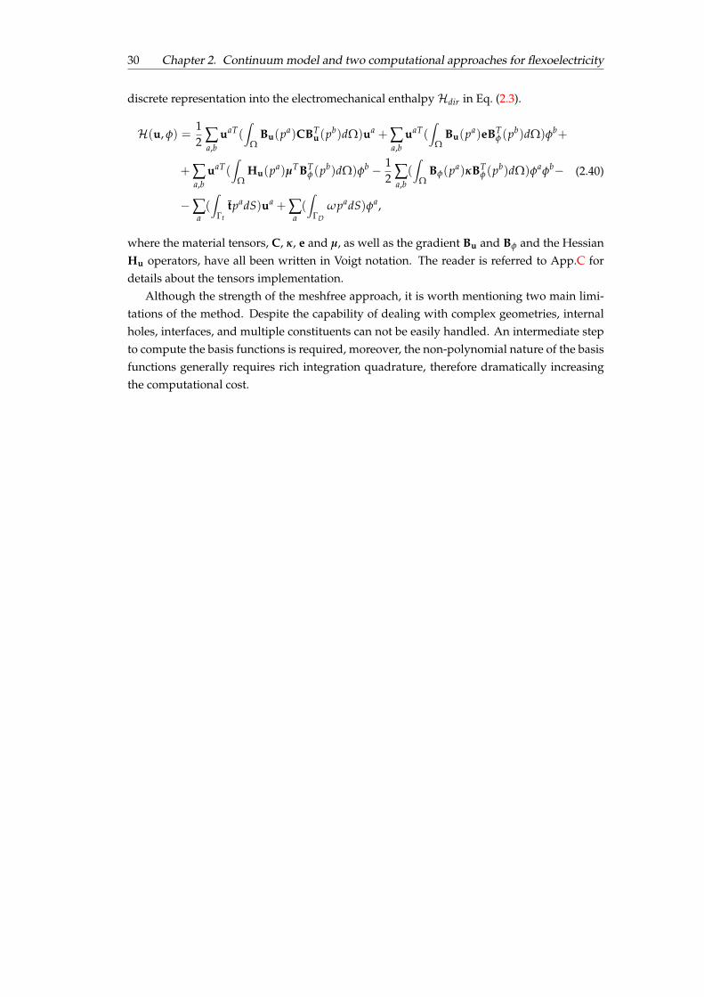
30 Chapter 2. Continuum model and two computational approaches for flexoelectricity
discrete representation into the electromechanical enthalpy Hdir in Eq. (2.3).
H(u, f) =12 Â
a,buaT(
Z
WBu(pa)CBT
u(pb)dW)ua + Âa,b
uaT(Z
WBu(pa)eBT
f(pb)dW)fb+
+ Âa,b
uaT(Z
WHu(pa)µTBT
f(pb)dW)fb � 12 Â
a,b(Z
WBf(pa)kBT
f(pb)dW)fafb�
� Âa(Z
GttpadS)ua + Â
a(Z
GDwpadS)fa,
(2.40)
where the material tensors, C, k, e and µ, as well as the gradient Bu and Bf and the HessianHu operators, have all been written in Voigt notation. The reader is referred to App.C fordetails about the tensors implementation.
Although the strength of the meshfree approach, it is worth mentioning two main limi-tations of the method. Despite the capability of dealing with complex geometries, internalholes, interfaces, and multiple constituents can not be easily handled. An intermediate stepto compute the basis functions is required, moreover, the non-polynomial nature of the basisfunctions generally requires rich integration quadrature, therefore dramatically increasingthe computational cost.
31
Chapter 3
Flexoelectricity-based piezoelectricmetamaterials and devices
3.1 Introduction
In 1968 Veselago theoretically proposed an engineered material with negative magnetic per-meability and electric permittivity able to exhibit special macroscopic properties as negativerefraction or backward wave propagation [93]. The name used to refer to this new classof material was left-handed material (LHM). Only later, in 1999, the definition of the termmetamaterial was minted. Nowadays, a metamaterial can be defined as "a macroscopic com-posite of periodic or non-periodic structure, whose function is due to both the cellular architectureand the chemical composition"[94]. Therefore, metamaterials can be considered a class of ma-terial properly engineered to produce properties that do not occur naturally or to enhanceintrinsic material properties. Mainly, due to progress in nano-technologies and experiments,in the last decades, many headways have been done in this promising field. Ranging fromwave manipulation in electromagnetism [95–98], optics [99] and acoustic [100], to stiffnessand lightness control in mechanics and structural applications [101–104], the spectrum ofpossibilities for new functionalities and extended material properties is in the thick of itsoutgrowth, especially for multiphysics coupling effects.
Many technologies involving sensing [2, 105], actuation [4] and energy harvesting [1, 3,106, 107] rely on the ability of some materials to transduce electrical fields into mechanicaldeformation and vice-versa. This ability, as previously discussed, is generally physicallysupported by the piezoelectric effect [108]. The best-known piezoelectrics are ferroelec-tric ceramics, which are ubiquitous in current technologies despite their several downsides.The most efficient piezoelectrics, such as Lead-Zirconate-Titanate (PZT), consist of lead foraround 60% of their entire composition. Substantial amounts of toxic substances are releasedduring the manufacturing stage, moreover, the high percentage of hazardous substances ren-ders the device not bio-compatible and certainly inapt for biomedical applications. In thisregard, since 2003 the European Union has imposed restrictions and requested the replace-ment of hazardous substances from electric and electronic devices in favor of lead-free mate-rials. The commitment of the scientific community in this field is synthesized in Fig. 3.1. Dueto their own nature, piezoelectric materials also exhibit a very low elastic modulus (around70GPa), which renders the materials extremely brittle with a toughness comparable withthat of windows glass [6]. A further disadvantage is related to their restricted range of oper-ating temperature limited by the Curie temperature (tc), above which many of them becomecentrosymmetric, thus losing their piezoelectric properties altogether [6, 7, 9, 10, 109–111].
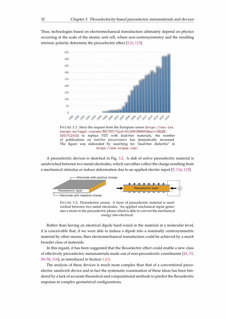
32 Chapter 3. Flexoelectricity-based piezoelectric metamaterials and devices
Thus, technologies based on electromechanical transduction ultimately depend on physicsoccurring at the scale of the atomic unit cell, where non-centrosymmetry and the resultingintrinsic polarity determine the piezoelectric effect [112, 113].
FIGURE 3.1: Since the request from the European union (https://eur-lex.europa.eu/legal-content/EN/TXT/?qid=1512061986553&uri=CELEX:32017L2102) to replace PZT with lead-free materials, the numberof publications on lead-free piezoceramics has dramatically increased.The figure was elaborated by searching for "lead-free dielectric" in
https://www.scopus.com/.
A piezoelectric devices is sketched in Fig. 3.2. A slab of active piezoelectric material issandwiched between two metal electrodes, which can either collect the charge resulting froma mechanical stimulus or induce deformation due to an applied electric input [5, 114, 115].
Piezoelectric layer Electrode with negative charge
Electrode with positive charge
V+ + + + + + + +
- - - - - - - -Piezoelectric layer
FIGURE 3.2: Piezoelectric sensor. A layer of piezoelectric material is sand-wiched between two metal electrodes. An applied mechanical input gener-ates a strain in the piezoelectric phase which is able to convert the mechanical
energy into electrical.
Rather than having an electrical dipole hard-wired in the material at a molecular level,it is conceivable that, if we were able to induce a dipole into a nominally centrosymmetricmaterial by other means, then electromechanical transduction could be achieved by a muchbroader class of materials.
In this regard, it has been suggested that the flexoelectric effect could enable a new classof effectively piezoelectric metamaterials made out of non-piezoelectric constituents [41, 53,56–58, 116], as introduced in Section 1.2.3.
The analysis of these devices is much more complex than that of a conventional piezo-electric sandwich device and in fact the systematic examination of these ideas has been hin-dered by a lack of accurate theoretical and computational methods to predict the flexoelectricresponse in complex geometrical configurations.
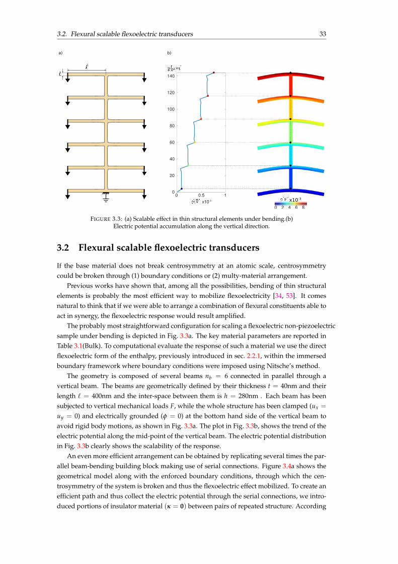
3.2. Flexural scalable flexoelectric transducers 33
a) b)
0
140
120
100
80
60
40
20
0
0 42 6 8x10⁻³
0.5 1x10⁻³
FIGURE 3.3: (a) Scalable effect in thin structural elements under bending.(b)Electric potential accumulation along the vertical direction.
3.2 Flexural scalable flexoelectric transducers
If the base material does not break centrosymmetry at an atomic scale, centrosymmetrycould be broken through (1) boundary conditions or (2) multy-material arrangement.
Previous works have shown that, among all the possibilities, bending of thin structuralelements is probably the most efficient way to mobilize flexoelectricity [34, 53]. It comesnatural to think that if we were able to arrange a combination of flexural constituents able toact in synergy, the flexoelectric response would result amplified.
The probably most straightforward configuration for scaling a flexoelectric non-piezoelectricsample under bending is depicted in Fig. 3.3a. The key material parameters are reported inTable 3.1(Bulk). To computational evaluate the response of such a material we use the directflexoelectric form of the enthalpy, previously introduced in sec. 2.2.1, within the immersedboundary framework where boundary conditions were imposed using Nitsche’s method.
The geometry is composed of several beams nb = 6 connected in parallel through avertical beam. The beams are geometrically defined by their thickness t = 40nm and theirlength ` = 400nm and the inter-space between them is h = 280nm . Each beam has beensubjected to vertical mechanical loads F, while the whole structure has been clamped (ux =
uy = 0) and electrically grounded (f = 0) at the bottom hand side of the vertical beam toavoid rigid body motions, as shown in Fig. 3.3a. The plot in Fig. 3.3b, shows the trend of theelectric potential along the mid-point of the vertical beam. The electric potential distributionin Fig. 3.3b clearly shows the scalability of the response.
An even more efficient arrangement can be obtained by replicating several times the par-allel beam-bending building block making use of serial connections. Figure 3.4a shows thegeometrical model along with the enforced boundary conditions, through which the cen-trosymmetry of the system is broken and thus the flexoelectric effect mobilized. To create anefficient path and thus collect the electric potential through the serial connections, we intro-duced portions of insulator material (k = 0) between pairs of repeated structure. According
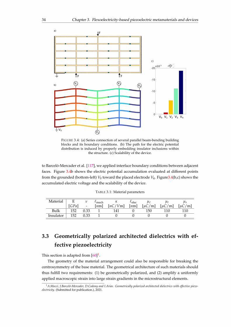
34 Chapter 3. Flexoelectricity-based piezoelectric metamaterials and devices
c)
-5
-10
-15
-20x10-3
0V0 V1 V2 V3 V4
a)
F F
F
b)
V0 V2
V3 V4V1
FIGURE 3.4: (a) Series connection of several parallel beam-bending buildingblocks and its boundary conditions. (b) The path for the electric potentialdistribution is induced by properly embedding insulator inclusions within
the structure. (c) Scalability of the device.
to Barceló-Mercader et al. [117], we applied interface boundary conditions between adjacentfaces. Figure 3.4b shows the electric potential accumulation evaluated at different pointsfrom the grounded (bottom-left) V0 toward the placed electrode V4. Figure3.4(b,c) shows theaccumulated electric voltage and the scalability of the device.
TABLE 3.1: Material parameters
Material E n `mech k `elec µ` µt µs[GPa] - [nm] [nC/Vm] [nm] [µC/m] [µC/m] [µC/m]
Bulk 152 0.33 1 141 0 150 110 110Insulator 152 0.33 1 0 0 0 0 0
3.3 Geometrically polarized architected dielectrics with ef-fective piezoelectricity
This section is adapted from [60]1.The geometry of the material arrangement could also be responsible for breaking the
centrosymmetry of the base material. The geometrical architecture of such materials shouldthus fulfill two requirements: (1) be geometrically polarized, and (2) amplify a uniformlyapplied macroscopic strain into large strain gradients in the microstructural elements.
1A.Mocci, J.Barceló-Mercader, D.Codony and I.Arias. Geometrically polarized architected dielectrics with effective piezo-electricity. (Submitted for publication.), 2021.
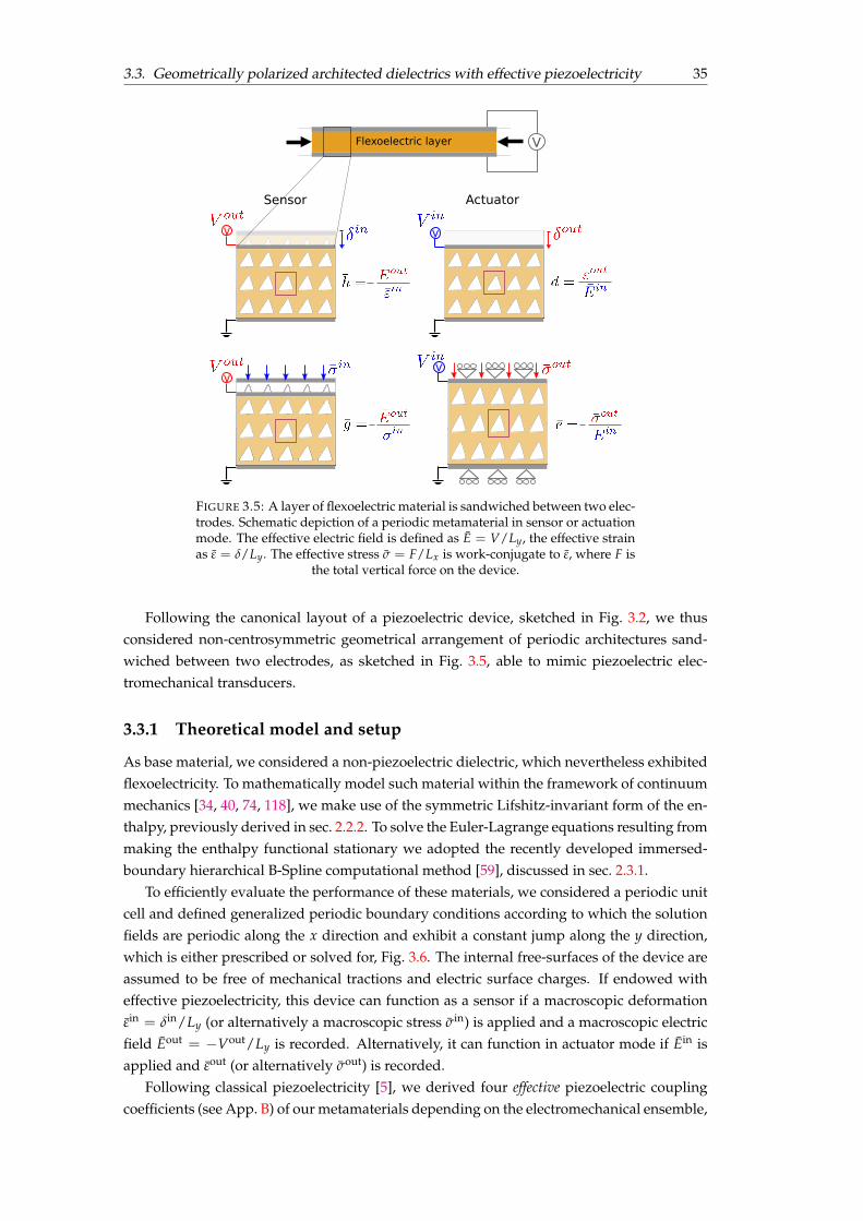
3.3. Geometrically polarized architected dielectrics with effective piezoelectricity 35
VFlexoelectric layer
V
V
Sensor
V
V
Actuator
FIGURE 3.5: A layer of flexoelectric material is sandwiched between two elec-trodes. Schematic depiction of a periodic metamaterial in sensor or actuationmode. The effective electric field is defined as E = V/Ly, the effective strainas # = d/Ly. The effective stress s = F/Lx is work-conjugate to #, where F is
the total vertical force on the device.
Following the canonical layout of a piezoelectric device, sketched in Fig. 3.2, we thusconsidered non-centrosymmetric geometrical arrangement of periodic architectures sand-wiched between two electrodes, as sketched in Fig. 3.5, able to mimic piezoelectric elec-tromechanical transducers.
3.3.1 Theoretical model and setup
As base material, we considered a non-piezoelectric dielectric, which nevertheless exhibitedflexoelectricity. To mathematically model such material within the framework of continuummechanics [34, 40, 74, 118], we make use of the symmetric Lifshitz-invariant form of the en-thalpy, previously derived in sec. 2.2.2. To solve the Euler-Lagrange equations resulting frommaking the enthalpy functional stationary we adopted the recently developed immersed-boundary hierarchical B-Spline computational method [59], discussed in sec. 2.3.1.
To efficiently evaluate the performance of these materials, we considered a periodic unitcell and defined generalized periodic boundary conditions according to which the solutionfields are periodic along the x direction and exhibit a constant jump along the y direction,which is either prescribed or solved for, Fig. 3.6. The internal free-surfaces of the device areassumed to be free of mechanical tractions and electric surface charges. If endowed witheffective piezoelectricity, this device can function as a sensor if a macroscopic deformation#in = din/Ly (or alternatively a macroscopic stress sin) is applied and a macroscopic electricfield Eout = �Vout/Ly is recorded. Alternatively, it can function in actuator mode if Ein isapplied and #out (or alternatively sout) is recorded.
Following classical piezoelectricity [5], we derived four effective piezoelectric couplingcoefficients (see App. B) of our metamaterials depending on the electromechanical ensemble,
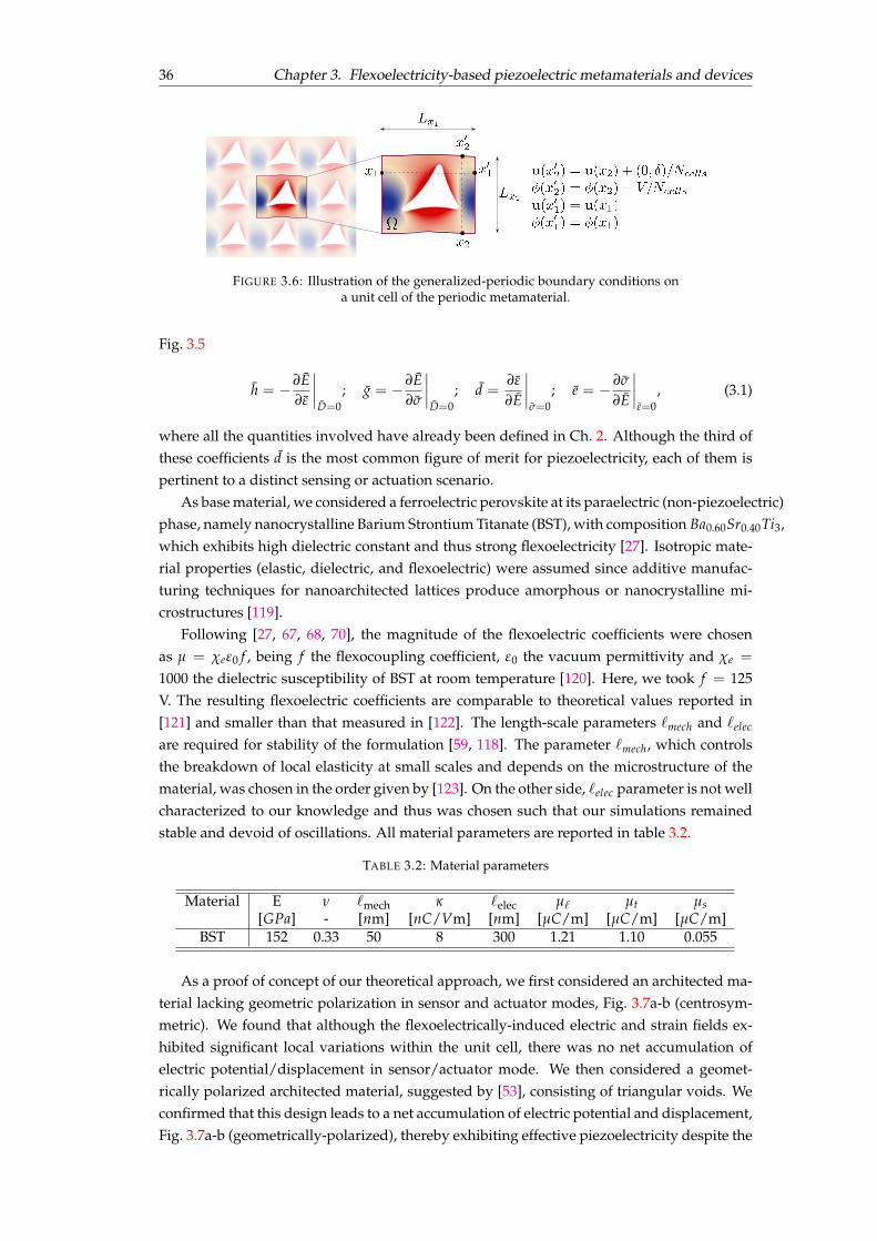
36 Chapter 3. Flexoelectricity-based piezoelectric metamaterials and devices
FIGURE 3.6: Illustration of the generalized-periodic boundary conditions ona unit cell of the periodic metamaterial.
Fig. 3.5
h = �∂E∂#
����D=0
; g = �∂E∂s
����D=0
; d =∂#
∂E
����s=0
; e = � ∂s
∂E
����#=0
, (3.1)
where all the quantities involved have already been defined in Ch. 2. Although the third ofthese coefficients d is the most common figure of merit for piezoelectricity, each of them ispertinent to a distinct sensing or actuation scenario.
As base material, we considered a ferroelectric perovskite at its paraelectric (non-piezoelectric)phase, namely nanocrystalline Barium Strontium Titanate (BST), with composition Ba0.60Sr0.40Ti3,which exhibits high dielectric constant and thus strong flexoelectricity [27]. Isotropic mate-rial properties (elastic, dielectric, and flexoelectric) were assumed since additive manufac-turing techniques for nanoarchitected lattices produce amorphous or nanocrystalline mi-crostructures [119].
Following [27, 67, 68, 70], the magnitude of the flexoelectric coefficients were chosenas µ = ce#0 f , being f the flexocoupling coefficient, #0 the vacuum permittivity and ce =
1000 the dielectric susceptibility of BST at room temperature [120]. Here, we took f = 125V. The resulting flexoelectric coefficients are comparable to theoretical values reported in[121] and smaller than that measured in [122]. The length-scale parameters `mech and `elec
are required for stability of the formulation [59, 118]. The parameter `mech, which controlsthe breakdown of local elasticity at small scales and depends on the microstructure of thematerial, was chosen in the order given by [123]. On the other side, `elec parameter is not wellcharacterized to our knowledge and thus was chosen such that our simulations remainedstable and devoid of oscillations. All material parameters are reported in table 3.2.
TABLE 3.2: Material parameters
Material E n `mech k `elec µ` µt µs[GPa] - [nm] [nC/Vm] [nm] [µC/m] [µC/m] [µC/m]
BST 152 0.33 50 8 300 1.21 1.10 0.055
As a proof of concept of our theoretical approach, we first considered an architected ma-terial lacking geometric polarization in sensor and actuator modes, Fig. 3.7a-b (centrosym-metric). We found that although the flexoelectrically-induced electric and strain fields ex-hibited significant local variations within the unit cell, there was no net accumulation ofelectric potential/displacement in sensor/actuator mode. We then considered a geomet-rically polarized architected material, suggested by [53], consisting of triangular voids. Weconfirmed that this design leads to a net accumulation of electric potential and displacement,Fig. 3.7a-b (geometrically-polarized), thereby exhibiting effective piezoelectricity despite the
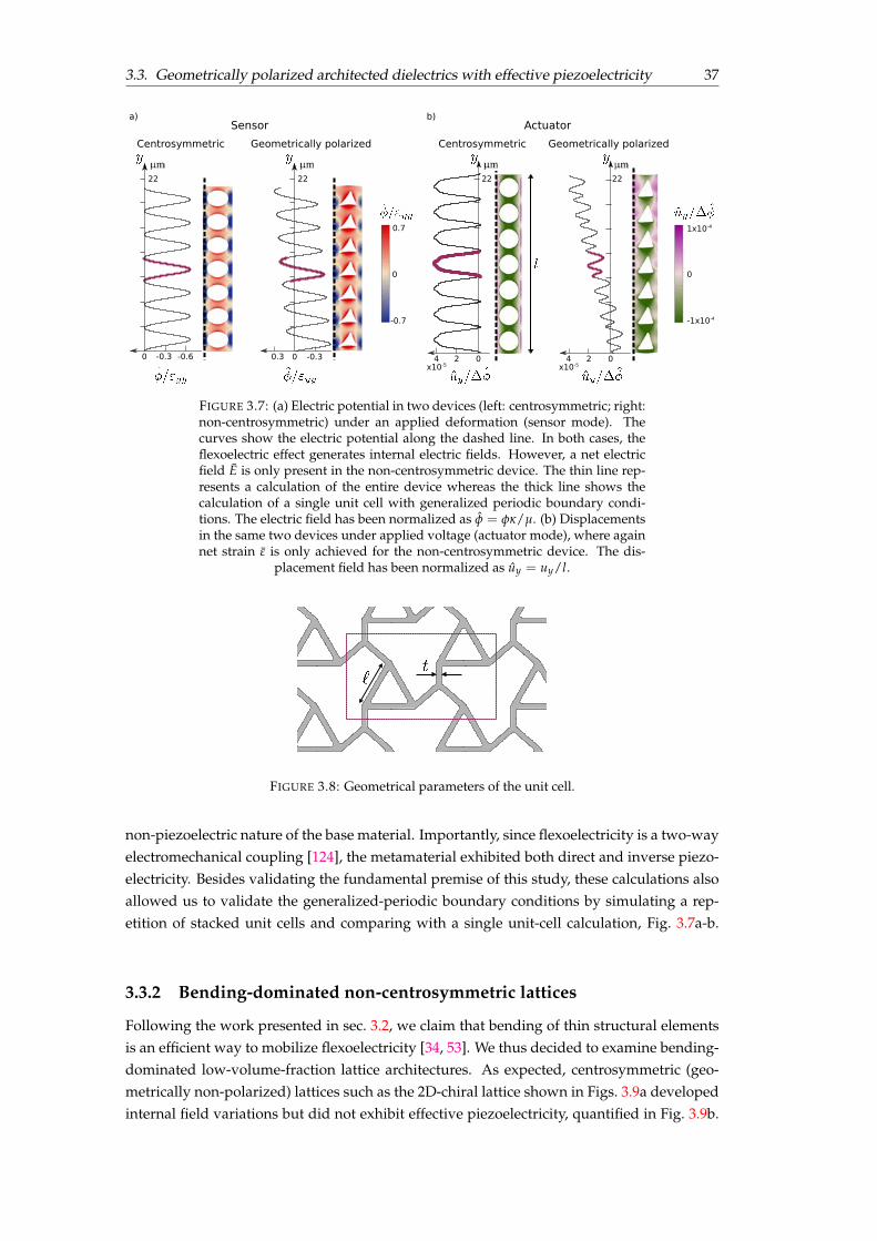
3.3. Geometrically polarized architected dielectrics with effective piezoelectricity 37
a)Sensor
Geometrically polarizedCentrosymmetric
-0.7
0
0.7
0.3 -0.30-0.3 -0.60
b)Actuator
Geometrically polarized
-1x10⁻⁴
0
1x10⁻⁴
4x10⁻⁵
2 0
Centrosymmetric
4x10⁻⁵
2 0
22222222
FIGURE 3.7: (a) Electric potential in two devices (left: centrosymmetric; right:non-centrosymmetric) under an applied deformation (sensor mode). Thecurves show the electric potential along the dashed line. In both cases, theflexoelectric effect generates internal electric fields. However, a net electricfield E is only present in the non-centrosymmetric device. The thin line rep-resents a calculation of the entire device whereas the thick line shows thecalculation of a single unit cell with generalized periodic boundary condi-tions. The electric field has been normalized as f = fk/µ. (b) Displacementsin the same two devices under applied voltage (actuator mode), where againnet strain # is only achieved for the non-centrosymmetric device. The dis-
placement field has been normalized as uy = uy/l.
FIGURE 3.8: Geometrical parameters of the unit cell.
non-piezoelectric nature of the base material. Importantly, since flexoelectricity is a two-wayelectromechanical coupling [124], the metamaterial exhibited both direct and inverse piezo-electricity. Besides validating the fundamental premise of this study, these calculations alsoallowed us to validate the generalized-periodic boundary conditions by simulating a rep-etition of stacked unit cells and comparing with a single unit-cell calculation, Fig. 3.7a-b.
3.3.2 Bending-dominated non-centrosymmetric lattices
Following the work presented in sec. 3.2, we claim that bending of thin structural elementsis an efficient way to mobilize flexoelectricity [34, 53]. We thus decided to examine bending-dominated low-volume-fraction lattice architectures. As expected, centrosymmetric (geo-metrically non-polarized) lattices such as the 2D-chiral lattice shown in Figs. 3.9a developedinternal field variations but did not exhibit effective piezoelectricity, quantified in Fig. 3.9b.
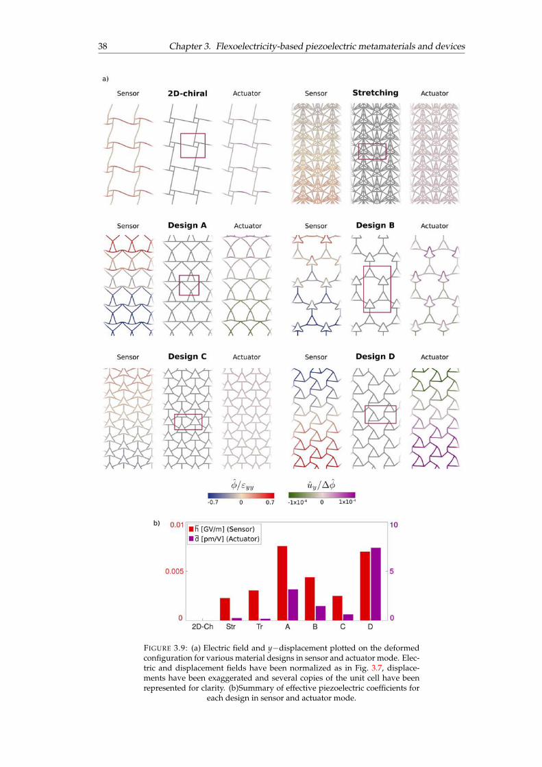
38 Chapter 3. Flexoelectricity-based piezoelectric metamaterials and devices
FIGURE 3.9: (a) Electric field and y�displacement plotted on the deformedconfiguration for various material designs in sensor and actuator mode. Elec-tric and displacement fields have been normalized as in Fig. 3.7, displace-ments have been exaggerated and several copies of the unit cell have beenrepresented for clarity. (b)Summary of effective piezoelectric coefficients for
each design in sensor and actuator mode.
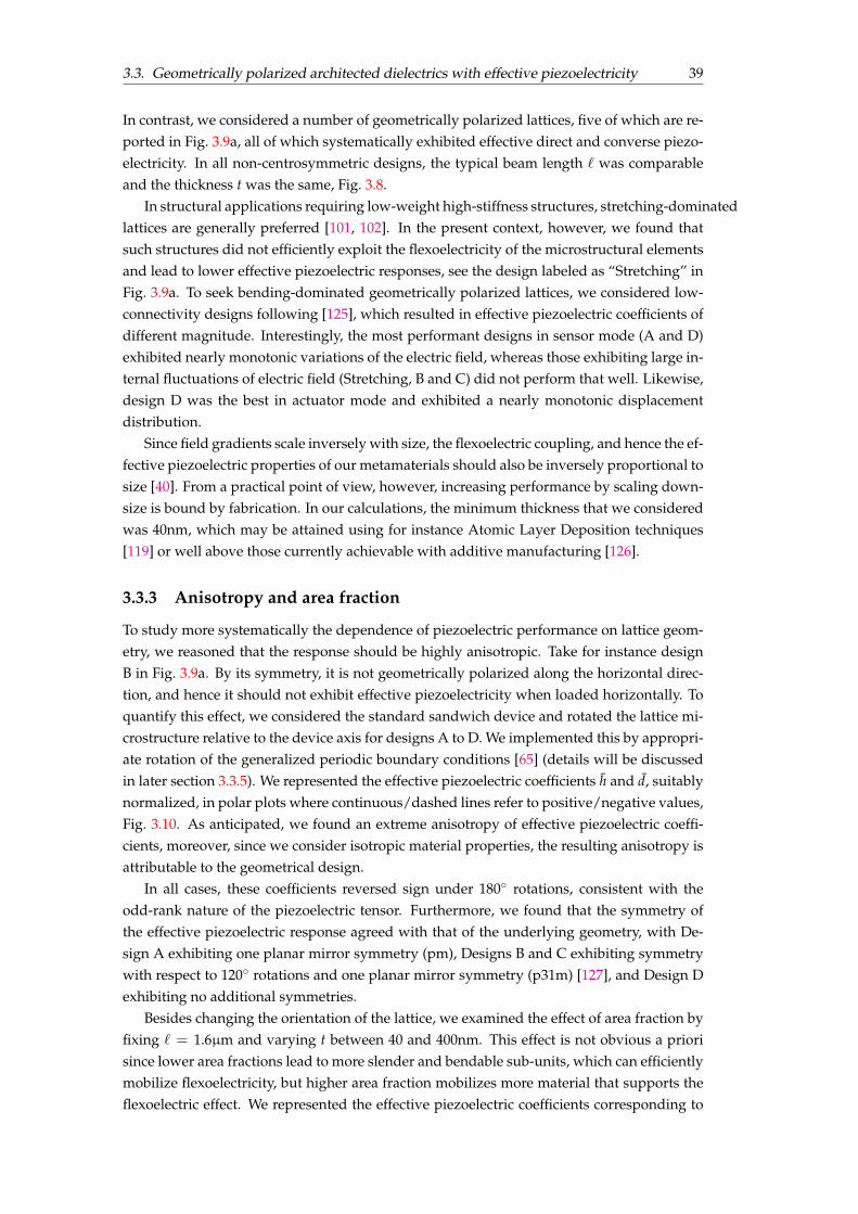
3.3. Geometrically polarized architected dielectrics with effective piezoelectricity 39
In contrast, we considered a number of geometrically polarized lattices, five of which are re-ported in Fig. 3.9a, all of which systematically exhibited effective direct and converse piezo-electricity. In all non-centrosymmetric designs, the typical beam length ` was comparableand the thickness t was the same, Fig. 3.8.
In structural applications requiring low-weight high-stiffness structures, stretching-dominatedlattices are generally preferred [101, 102]. In the present context, however, we found thatsuch structures did not efficiently exploit the flexoelectricity of the microstructural elementsand lead to lower effective piezoelectric responses, see the design labeled as “Stretching” inFig. 3.9a. To seek bending-dominated geometrically polarized lattices, we considered low-connectivity designs following [125], which resulted in effective piezoelectric coefficients ofdifferent magnitude. Interestingly, the most performant designs in sensor mode (A and D)exhibited nearly monotonic variations of the electric field, whereas those exhibiting large in-ternal fluctuations of electric field (Stretching, B and C) did not perform that well. Likewise,design D was the best in actuator mode and exhibited a nearly monotonic displacementdistribution.
Since field gradients scale inversely with size, the flexoelectric coupling, and hence the ef-fective piezoelectric properties of our metamaterials should also be inversely proportional tosize [40]. From a practical point of view, however, increasing performance by scaling down-size is bound by fabrication. In our calculations, the minimum thickness that we consideredwas 40nm, which may be attained using for instance Atomic Layer Deposition techniques[119] or well above those currently achievable with additive manufacturing [126].
3.3.3 Anisotropy and area fraction
To study more systematically the dependence of piezoelectric performance on lattice geom-etry, we reasoned that the response should be highly anisotropic. Take for instance designB in Fig. 3.9a. By its symmetry, it is not geometrically polarized along the horizontal direc-tion, and hence it should not exhibit effective piezoelectricity when loaded horizontally. Toquantify this effect, we considered the standard sandwich device and rotated the lattice mi-crostructure relative to the device axis for designs A to D. We implemented this by appropri-ate rotation of the generalized periodic boundary conditions [65] (details will be discussedin later section 3.3.5). We represented the effective piezoelectric coefficients h and d, suitablynormalized, in polar plots where continuous/dashed lines refer to positive/negative values,Fig. 3.10. As anticipated, we found an extreme anisotropy of effective piezoelectric coeffi-cients, moreover, since we consider isotropic material properties, the resulting anisotropy isattributable to the geometrical design.
In all cases, these coefficients reversed sign under 180� rotations, consistent with theodd-rank nature of the piezoelectric tensor. Furthermore, we found that the symmetry ofthe effective piezoelectric response agreed with that of the underlying geometry, with De-sign A exhibiting one planar mirror symmetry (pm), Designs B and C exhibiting symmetrywith respect to 120� rotations and one planar mirror symmetry (p31m) [127], and Design Dexhibiting no additional symmetries.
Besides changing the orientation of the lattice, we examined the effect of area fraction byfixing ` = 1.6µm and varying t between 40 and 400nm. This effect is not obvious a priorisince lower area fractions lead to more slender and bendable sub-units, which can efficientlymobilize flexoelectricity, but higher area fraction mobilizes more material that supports theflexoelectric effect. We represented the effective piezoelectric coefficients corresponding to
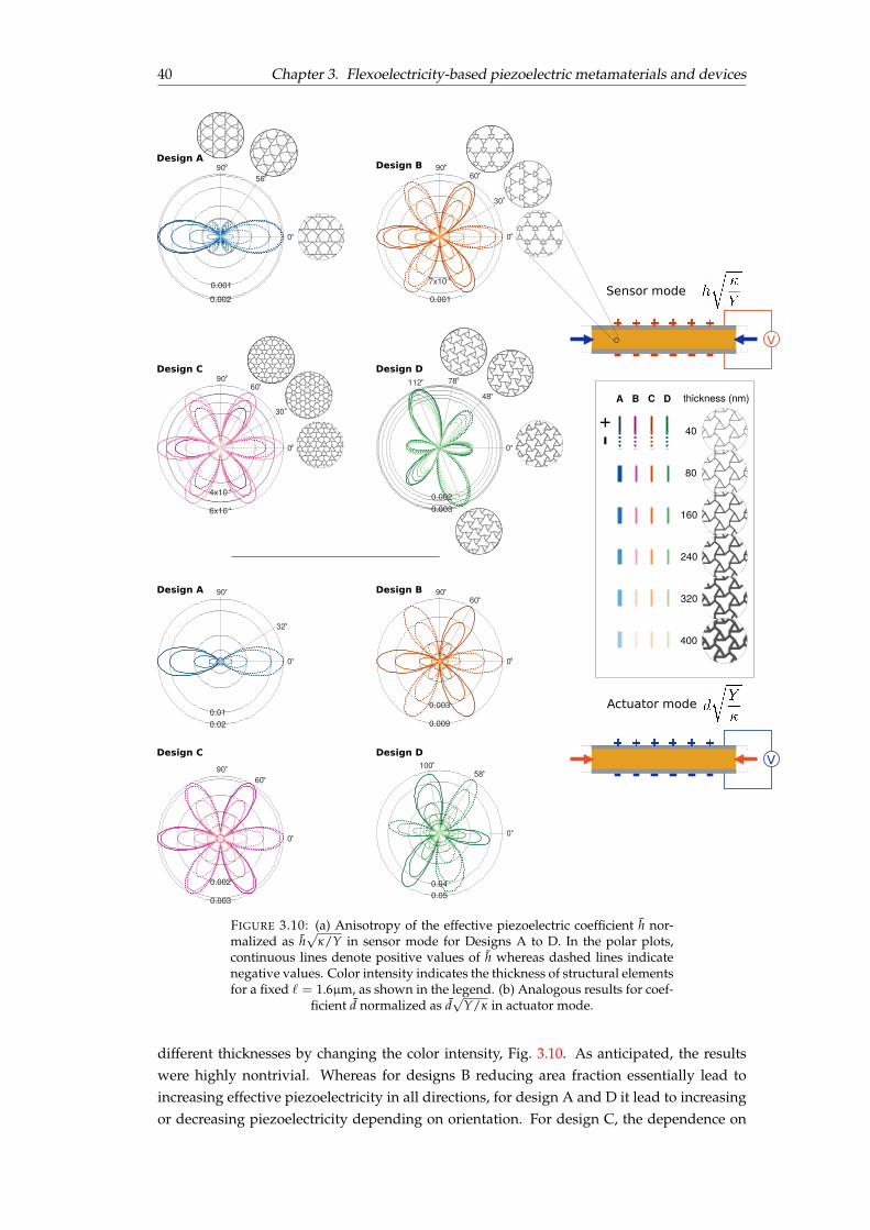
40 Chapter 3. Flexoelectricity-based piezoelectric metamaterials and devices
Sensor mode
V+ + + + + +
- - - - - -
Actuator mode
V+ + + + + +
- - - - - -
+-
A CB D thickness (nm)
40
80
160
240
320
400
Design A
0
90
0.0020.001
56
Design B 60
90
0
30
0.001
7x10⁻⁴
Design C 60
90
0
30
6x10⁻⁴
4x10⁻⁴
Design D
48
0
112
78
0.0030.002
Design A
0
90
32
0.020.01
Design B 60
90
0
0.009
0.003
Design C
60
90
0
0.003
0.002
Design D
58
0
100
0.050.04
FIGURE 3.10: (a) Anisotropy of the effective piezoelectric coefficient h nor-malized as h
pk/Y in sensor mode for Designs A to D. In the polar plots,
continuous lines denote positive values of h whereas dashed lines indicatenegative values. Color intensity indicates the thickness of structural elementsfor a fixed ` = 1.6µm, as shown in the legend. (b) Analogous results for coef-
ficient d normalized as dp
Y/k in actuator mode.
different thicknesses by changing the color intensity, Fig. 3.10. As anticipated, the resultswere highly nontrivial. Whereas for designs B reducing area fraction essentially lead toincreasing effective piezoelectricity in all directions, for design A and D it lead to increasingor decreasing piezoelectricity depending on orientation. For design C, the dependence on
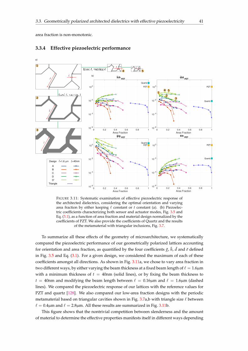
3.3. Geometrically polarized architected dielectrics with effective piezoelectricity 41
area fraction is non-monotonic.
3.3.4 Effective piezoelectric performance
h/h PZT
0 0.2 0.4 0.6 0.8 1Area Fraction
10 -6
10 -4
10 -2
10 0Quartz
PZT
g/g PZT
0 0.2 0.4 0.6 0.8 1Area Fraction
10 -6
10 -4
10 -2
10 0Quartz
PZT
d/d PZT
0 0.2 0.4 0.6 0.8 1Area Fraction
10 -6
10 -4
10 -2
10 0
Quartz
PZT
12
3
4 5
0 0.2 0.4 0.6 0.8 1Area Fraction
10 -6
10 -4
10 -2
10 0
Quartz
PZT
e/e PZT
a)
b)
4 51
3
2
Design =40nm
CD
BA
µm=1.6
TriangleD'
FIGURE 3.11: Systematic examination of effective piezoelectric response ofthe architected dielectrics, considering the optimal orientation and varyingarea fraction by either keeping ` constant or t constant (a). (b) Piezoelec-tric coefficients characterizing both sensor and actuator modes, Fig. 3.5 andEq. (3.1), as a function of area fraction and material design normalized by thecoefficients of PZT. We also provide the coefficients of Quartz and the results
of the metamaterial with triangular inclusions, Fig. 3.7.
To summarize all these effects of the geometry of microarchitecture, we systematicallycompared the piezoelectric performance of our geometrically polarized lattices accountingfor orientation and area fraction, as quantified by the four coefficients g, h, d and e definedin Fig. 3.5 and Eq. (3.1). For a given design, we considered the maximum of each of thesecoefficients amongst all directions. As shown in Fig. 3.11a, we chose to vary area fraction intwo different ways, by either varying the beam thickness at a fixed beam length of ` = 1.6µmwith a minimum thickness of t = 40nm (solid lines), or by fixing the beam thickness tot = 40nm and modifying the beam length between ` = 0.16µm and ` = 1.6µm (dashedlines). We compared the piezoelectric response of our lattices with the reference values forPZT and quartz [128]. We also compared our low-area fraction designs with the periodicmetamaterial based on triangular cavities shown in Fig. 3.7a,b with triangle size ` between` = 0.4µm and ` = 2.8µm. All these results are summarized in Fig. 3.11b.
This figure shows that the nontrivial competition between slenderness and the amountof material to determine the effective properties manifests itself in different ways depending
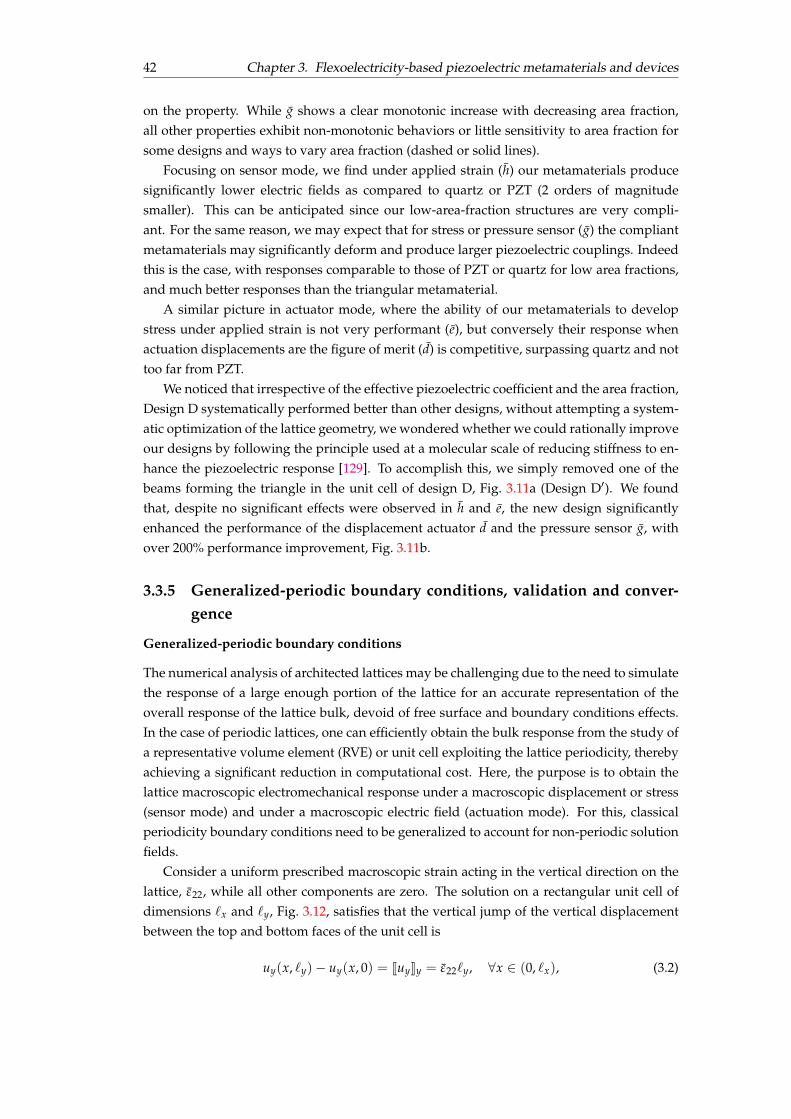
42 Chapter 3. Flexoelectricity-based piezoelectric metamaterials and devices
on the property. While g shows a clear monotonic increase with decreasing area fraction,all other properties exhibit non-monotonic behaviors or little sensitivity to area fraction forsome designs and ways to vary area fraction (dashed or solid lines).
Focusing on sensor mode, we find under applied strain (h) our metamaterials producesignificantly lower electric fields as compared to quartz or PZT (2 orders of magnitudesmaller). This can be anticipated since our low-area-fraction structures are very compli-ant. For the same reason, we may expect that for stress or pressure sensor (g) the compliantmetamaterials may significantly deform and produce larger piezoelectric couplings. Indeedthis is the case, with responses comparable to those of PZT or quartz for low area fractions,and much better responses than the triangular metamaterial.
A similar picture in actuator mode, where the ability of our metamaterials to developstress under applied strain is not very performant (e), but conversely their response whenactuation displacements are the figure of merit (d) is competitive, surpassing quartz and nottoo far from PZT.
We noticed that irrespective of the effective piezoelectric coefficient and the area fraction,Design D systematically performed better than other designs, without attempting a system-atic optimization of the lattice geometry, we wondered whether we could rationally improveour designs by following the principle used at a molecular scale of reducing stiffness to en-hance the piezoelectric response [129]. To accomplish this, we simply removed one of thebeams forming the triangle in the unit cell of design D, Fig. 3.11a (Design D0). We foundthat, despite no significant effects were observed in h and e, the new design significantlyenhanced the performance of the displacement actuator d and the pressure sensor g, withover 200% performance improvement, Fig. 3.11b.
3.3.5 Generalized-periodic boundary conditions, validation and conver-gence
Generalized-periodic boundary conditions
The numerical analysis of architected lattices may be challenging due to the need to simulatethe response of a large enough portion of the lattice for an accurate representation of theoverall response of the lattice bulk, devoid of free surface and boundary conditions effects.In the case of periodic lattices, one can efficiently obtain the bulk response from the study ofa representative volume element (RVE) or unit cell exploiting the lattice periodicity, therebyachieving a significant reduction in computational cost. Here, the purpose is to obtain thelattice macroscopic electromechanical response under a macroscopic displacement or stress(sensor mode) and under a macroscopic electric field (actuation mode). For this, classicalperiodicity boundary conditions need to be generalized to account for non-periodic solutionfields.
Consider a uniform prescribed macroscopic strain acting in the vertical direction on thelattice, #22, while all other components are zero. The solution on a rectangular unit cell ofdimensions `x and `y, Fig. 3.12, satisfies that the vertical jump of the vertical displacementbetween the top and bottom faces of the unit cell is
uy(x, `y)� uy(x, 0) = JuyKy = #22`y, 8x 2 (0, `x), (3.2)
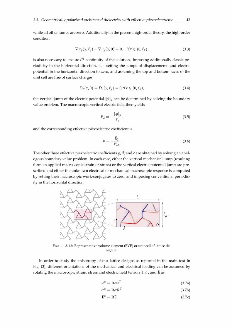
3.3. Geometrically polarized architected dielectrics with effective piezoelectricity 43
while all other jumps are zero. Additionally, in the present high-order theory, the high-ordercondition
ruy(x, `y)�ruy(x, 0) = 0, 8x 2 (0, `x). (3.3)
is also necessary to ensure C1 continuity of the solution. Imposing additionally classic pe-riodicity in the horizontal direction, i.e. setting the jumps of displacements and electricpotential in the horizontal direction to zero, and assuming the top and bottom faces of theunit cell are free of surface charges,
D2(x, 0) = D2(x, `y) = 0, 8x 2 (0, `x), (3.4)
the vertical jump of the electric potential JfKy can be determined by solving the boundaryvalue problem. The macroscopic vertical electric field then yields
E2 = �JfKy
`y, (3.5)
and the corresponding effective piezoelectric coefficient is
h = � E2#22
. (3.6)
The other three effective piezoelectric coefficients g, d, and e are obtained by solving an anal-ogous boundary value problem. In each case, either the vertical mechanical jump (resultingform an applied macroscopic strain or stress) or the vertical electric potential jump are pre-scribed and either the unknown electrical or mechanical macroscopic response is computedby setting their macroscopic work-conjugates to zero, and imposing conventional periodic-ity in the horizontal direction.
FIGURE 3.12: Representative volume element (RVE) or unit cell of lattice de-sign D.
In order to study the anisotropy of our lattice designs as reported in the main text inFig. (3), different orientations of the mechanical and electrical loading can be assumed byrotating the macroscopic strain, stress and electric field tensors #, s, and E as
#a = R#RT (3.7a)
sa = RsRT (3.7b)
Ea = RE (3.7c)
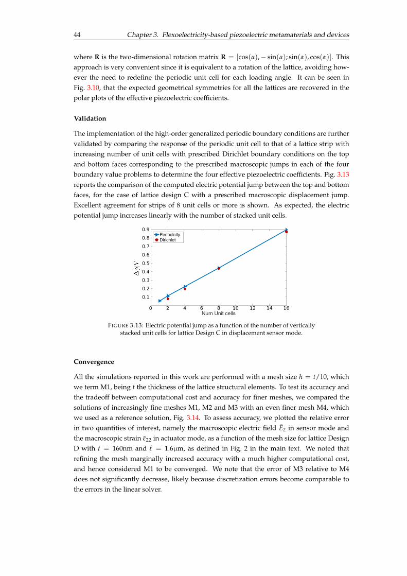
44 Chapter 3. Flexoelectricity-based piezoelectric metamaterials and devices
where R is the two-dimensional rotation matrix R = [cos(a),� sin(a); sin(a), cos(a)]. Thisapproach is very convenient since it is equivalent to a rotation of the lattice, avoiding how-ever the need to redefine the periodic unit cell for each loading angle. It can be seen inFig. 3.10, that the expected geometrical symmetries for all the lattices are recovered in thepolar plots of the effective piezoelectric coefficients.
Validation
The implementation of the high-order generalized periodic boundary conditions are furthervalidated by comparing the response of the periodic unit cell to that of a lattice strip withincreasing number of unit cells with prescribed Dirichlet boundary conditions on the topand bottom faces corresponding to the prescribed macroscopic jumps in each of the fourboundary value problems to determine the four effective piezoelectric coefficients. Fig. 3.13reports the comparison of the computed electric potential jump between the top and bottomfaces, for the case of lattice design C with a prescribed macroscopic displacement jump.Excellent agreement for strips of 8 unit cells or more is shown. As expected, the electricpotential jump increases linearly with the number of stacked unit cells.
Num Unit cells
PeriodicityDirichlet
0 2 4 6 8 10 12 14 16
0.10.20.30.40.50.60.70.80.9
FIGURE 3.13: Electric potential jump as a function of the number of verticallystacked unit cells for lattice Design C in displacement sensor mode.
Convergence
All the simulations reported in this work are performed with a mesh size h = t/10, whichwe term M1, being t the thickness of the lattice structural elements. To test its accuracy andthe tradeoff between computational cost and accuracy for finer meshes, we compared thesolutions of increasingly fine meshes M1, M2 and M3 with an even finer mesh M4, whichwe used as a reference solution, Fig. 3.14. To assess accuracy, we plotted the relative errorin two quantities of interest, namely the macroscopic electric field E2 in sensor mode andthe macroscopic strain #22 in actuator mode, as a function of the mesh size for lattice DesignD with t = 160nm and ` = 1.6µm, as defined in Fig. 2 in the main text. We noted thatrefining the mesh marginally increased accuracy with a much higher computational cost,and hence considered M1 to be converged. We note that the error of M3 relative to M4does not significantly decrease, likely because discretization errors become comparable tothe errors in the linear solver.
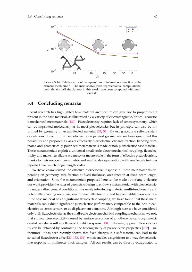
3.4. Concluding remarks 45
t/h
e RM1 M2 M3
15 20 25 30 35 4010 -6
10 -5
10 -4
FIGURE 3.14: Relative error of two quantities of interest as a function of theelement mesh size h. The inset shows three representative computationalmesh details. All simulations in this work have been computed with mesh
level M1.
3.4 Concluding remarks
Recent research has highlighted how material architecture can give rise to properties notpresent in the base material, as illustrated by a variety of electromagnetic/optical, acoustic,o mechanical metamaterials [130]. Piezoelectricity requires lack of centrosymmetry, whichcan be imprinted molecularly as in most piezoelectrics but in principle can also be im-printed by geometry in an architected material [53, 56]. By using accurate self-consistentcalculations of continuum flexoelectricity on general geometries, we have quantified thispossibility and proposed a class of effectively piezoelectric low area-fraction, bending dom-inated and geometrically-polarized metamaterials made of non-piezoelectric base material.These metamaterials exploit a universal small-scale electromechanical coupling, flexoelec-tricity, and make it available at a meso- or macro-scale in the form of effective piezoelectricitythanks to their non-centrosymmetric and multiscale organization, with small-scale featuresrepeated over much longer length scales.
We have characterized the effective piezoelectric response of these metamaterials de-pending on geometry, area-fraction at fixed thickness, area-fraction at fixed beam length,and orientation. Since the metamaterials proposed here can be made out of any dielectric,our work provides the rules of geometric design to endow a metamaterial with piezoelectric-ity under rather general conditions, thus easily introducing material multi-functionality andpotentially enabling non-toxic, environmentally friendly, and biocompatible piezoelectrics.If the base material has a significant flexoelectric coupling, we have found that these meta-materials can exhibit significant piezoelectric performance, comparable to the best piezo-electrics as stress sensors or as displacement actuators. Although here we have consideredonly bulk flexoelectricity as the small-scale electromechanical coupling mechanism, we notethat surface piezoelectricity caused by surface relaxation of an otherwise centrosymmetriccrystal can also result in a flexoelectric-like response [131]. Likewise, apparent flexoelectric-ity can be obtained by controlling the heterogeneity of piezoelectric properties [132]. Fur-thermore, it has been recently shown that fixed charges in a soft material can lead to theso-called flexoelectret effect [20, 133, 134], which enables a significant two-way flexoelectric-like response in millimeter-thick samples. All our results can be directly extrapolated to
46 Chapter 3. Flexoelectricity-based piezoelectric metamaterials and devices
these situations, hence broadening the scope of our geometrically-polarized architected di-electrics with effective piezoelectricity.
Our work provides a framework for rational material design to control the magnitude(Design D0) and anisotropy (Fig. 3.10) of effective piezoelectricity. The design of our meta-materials is amenable to systematic computational topology and shape optimization [135]and additive manufacturing [58, 102, 126, 136], and hence may provide an alternative routeto conventional piezoelectric material design at a molecular scale [129]. Furthermore, piezo-electricity and flexoelectricity may act constructively if our geometrically polarized latticesare built from an already piezoelectric material, thereby enhancing their effective piezoelec-tricity[30, 42].
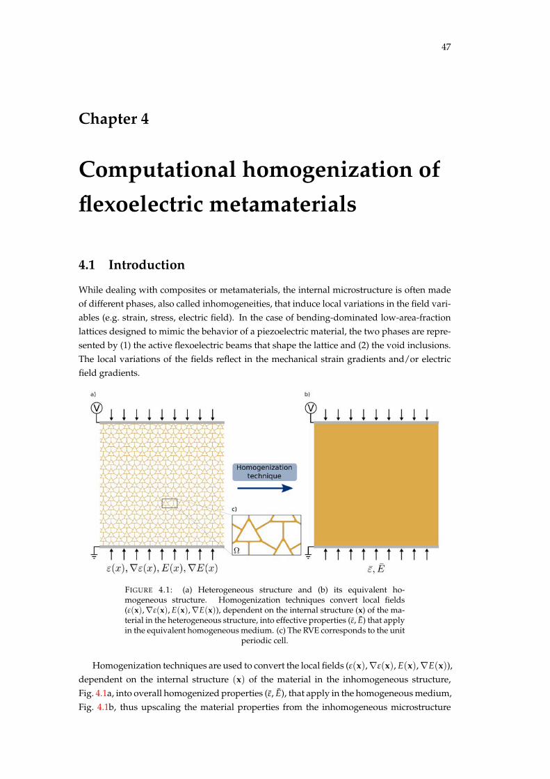
47
Chapter 4
Computational homogenization offlexoelectric metamaterials
4.1 Introduction
While dealing with composites or metamaterials, the internal microstructure is often madeof different phases, also called inhomogeneities, that induce local variations in the field vari-ables (e.g. strain, stress, electric field). In the case of bending-dominated low-area-fractionlattices designed to mimic the behavior of a piezoelectric material, the two phases are repre-sented by (1) the active flexoelectric beams that shape the lattice and (2) the void inclusions.The local variations of the fields reflect in the mechanical strain gradients and/or electricfield gradients.
FIGURE 4.1: (a) Heterogeneous structure and (b) its equivalent ho-mogeneous structure. Homogenization techniques convert local fields(#(x),r#(x), E(x),rE(x)), dependent on the internal structure (x) of the ma-terial in the heterogeneous structure, into effective properties (#, E) that applyin the equivalent homogeneous medium. (c) The RVE corresponds to the unit
periodic cell.
Homogenization techniques are used to convert the local fields (#(x),r#(x), E(x),rE(x)),dependent on the internal structure (x) of the material in the inhomogeneous structure,Fig. 4.1a, into overall homogenized properties (#, E), that apply in the homogeneous medium,Fig. 4.1b, thus upscaling the material properties from the inhomogeneous microstructure
48 Chapter 4. Computational homogenization of flexoelectric metamaterials
(i.e. where the flexoelectric constituents are described) to the macroscopic scale (i.e. thepiezoelectric homogenized medium). The computational domain is identified by the Repre-sentative Volume Element (RVE), which for periodic structures subjected to periodic bound-ary conditions corresponds to the unit periodic cell, as described in Ch. 3 and depicted inFig. 4.1c.
Several analytical and theoretical methods can be found in literature [137–139], howeverfor complex geometries and physics closed-form solutions are far from trivial, and compu-tational homogenization techniques are required.
In 1967, Adams [140] proposed a method to numerically characterize the macroscopicproperties of a composite from its local variations at the microscale. Although this approachis considered to be the first computational homogenization methodology in literature, it stillrepresents an extension of a simpler analytical approach. It is only in the late 1990s thatmore advanced computational homogenization methods are proposed to solve analyticallyunapproachable problems [141]. Nowadays, computational homogenization is used in awide variety of fields ranging from nonlinear [142], to fracture problems [143], to multi-physics and electromechanical coupled problems [144, 145]. Sharma et al. [53] proposed ahomogenization technique to solve an effective piezoelectric composite where nanoscale in-homogeneities were embedded within a flexoelectric matrix. The inhomogeneities, havingdifferent material properties with respect to the flexoelectric matrix, were treated as ficti-tious body forces and electric fields. In more recent work [132], a numerical homogenizationmethod was proposed to study the effect of heterogeneous piezoelectric composites able toendow the matrix with a flexoelectric-like response even though the base material has nosignificant flexoelectricity.
Based on this [146], here we propose a computational homogenization technique forflexoelectric-based metamaterials.
In Ch. 3 we presented some geometrically polarized metamaterials able to exploit theflexoelectric effect and behave as piezoelectric materials [60]. Although at a first stage wefocused on the characterization of the longitudinal piezoelectric modulus, i.e. the effective re-sponse along the loading direction with respect to the lattice orientation, the process of de-signing more conscious flexoelectric-based metamaterials passes through the awareness ofa comprehensive understanding of their enriched properties, reflected in the full character-ization of the effective macroscopic behavior and thus full evaluation of the homogenizedtensors, which is the contribution of this chapter [61]1.
4.2 Energy equivalence
The periodic unit cell in Fig. 4.1c subjected to periodic boundary conditions is treated as amaterial point for the homogeneous medium while generates local variations of the fields(#(x),r#(x), E(x),rE(x)) in its constituents. The base material is chosen to fit the behaviorof Barium Strontium Titanate (BST) above the Curie temperature in its paraelectric phase(non-piezoelectric), with composition Ba0.60Sr0.40Ti3, which exhibits high dielectric constantand thus strong flexoelectricity [27]. To model such a material we define the quadratic formof the electric enthalpy HhLi f i, introduced in sec. 2.2.2 and reported here to highlight thematerial coordinates x dependence of all the quantities involved, therefore implying that
1This chapter has been partially extrapolated from: A.Mocci,P.Gupta, and I.Arias. Shape optimization of architecteddielectrics with effective piezoelectricity using computational homogenization. (In Preparation).
4.2. Energy equivalence 49
inhomogeneities and local variations are captured by the enthalpy form.
HhLi f i(u, f) =12
#ij(x)Cijkl(x)#kl(x) +12
#ij,k(x)hijklmn(x)# lm,n(x)�12
f,l(x)klm(x)f,m(x)
� 12
f,mn(x)bmnlk(x)f,lk(x) +12
f,l(x)µlijk(x)#ij,k(x)�12
f,lk(x)µlijk(x)#ij(x).
(4.1)
The Euler-Lagrange equations, derived from the enthalpy function in Eq. (2.26), are thefourth-order coupled partial differential equations reported here for convenience:
(sij � sijk,k),j = 0 in W, (4.2a)
(Dl,l � Dlk,k),l = 0 in W. (4.2b)
where we have set the body forces b = 0 as well as the free electric charges q = 0.Following the Hill-Mandel theorem [147, 148], we make a hypothesis that the average of
the microscopic work done by the RVE must be equivalent to the macroscopic work done bythe fictitious homogeneous material. In order to prescribe this, we write the electric enthalpyof the equivalent piezoelectric medium (H) as the average of the electric enthalpy of theflexoelectric RVE (H).
H =
*H+
=12
#ijCijkl#kl � Elelij#ij �12
EikijEj, (4.3)
where h.i = 1VR(.)dV, with V being the RVE domain volume. By writing the energy in the
form of Eq. (4.3), the equilibrium equations turn out
sij,j = 0, Di,i = 0. (4.4)
Now, to prove our hypothesis in Eq. (4.3), we use Hill-Mandel theorem in which we firstlyconsider the mechanical work done by a flexoelectric metamaterial as
1V
Z
Vs
eqij #ij = sik#ik, (4.5)
where seqij = bsij � esijk,k is a statically admissible stress such that satisfies the equilibrium
equation seqij,j = 0 and #ij = 1/2(∂ui,j + ∂uj,i) a kinematically admissible strain, while the bar
quantities are the equivalent macroscopic stress and strain, respectively. Upon volume aver-aging the Eq. (4.2a) over the RVE domain by multiplying the variation in the displacementfield as
1V
Z
Vs
eqij,jdui dW =
1V
Z
V(s
eqij dui),j dW � 1
V
Z
Vs
eqij dui,j dW = 0, (4.6)
where W is the domain defining the RVE of our architected material. By applying divergencetheorem, we write
1V
Z
Gs
eqij duinj dG � 1
V
Z
Vs
eqij
✓12(dui,j + duj,i) +
12(dui,j � duj,i)
◆dW = 0. (4.7)
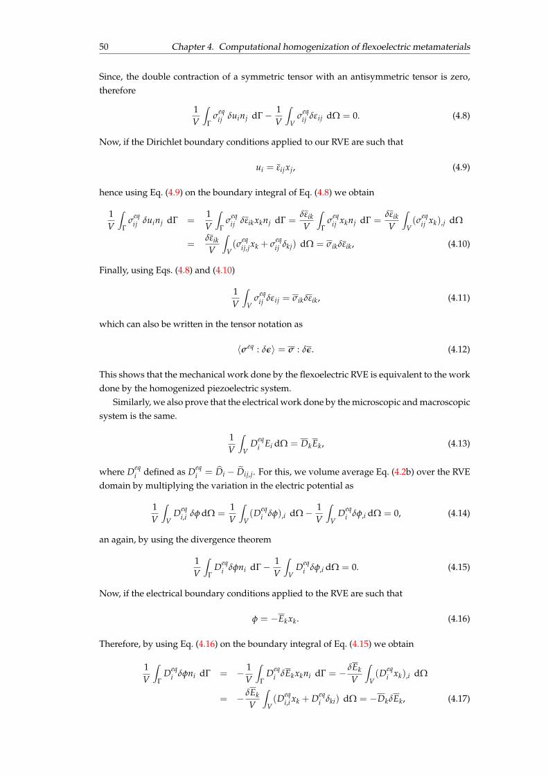
50 Chapter 4. Computational homogenization of flexoelectric metamaterials
Since, the double contraction of a symmetric tensor with an antisymmetric tensor is zero,therefore
1V
Z
Gs
eqij duinj dG � 1
V
Z
Vs
eqij d#ij dW = 0. (4.8)
Now, if the Dirichlet boundary conditions applied to our RVE are such that
ui = #ijxj, (4.9)
hence using Eq. (4.9) on the boundary integral of Eq. (4.8) we obtain
1V
Z
Gs
eqij duinj dG =
1V
Z
Gs
eqij d#ikxknj dG =
d#ikV
Z
Gs
eqij xknj dG =
d#ikV
Z
V(s
eqij xk),j dW
=d#ikV
Z
V(s
eqij,jxk + s
eqij dkj) dW = sikd#ik, (4.10)
Finally, using Eqs. (4.8) and (4.10)
1V
Z
Vs
eqij d#ij = sikd#ik, (4.11)
which can also be written in the tensor notation as
hseq : dei = s : de. (4.12)
This shows that the mechanical work done by the flexoelectric RVE is equivalent to the workdone by the homogenized piezoelectric system.
Similarly, we also prove that the electrical work done by the microscopic and macroscopicsystem is the same.
1V
Z
VDeq
i Ei dW = DkEk, (4.13)
where Deqi defined as Deq
i = bDi � eDij,j. For this, we volume average Eq. (4.2b) over the RVEdomain by multiplying the variation in the electric potential as
1V
Z
VDeq
i,i df dW =1V
Z
V(Deq
i df),i dW � 1V
Z
VDeq
i df,i dW = 0, (4.14)
an again, by using the divergence theorem
1V
Z
GDeq
i dfni dG � 1V
Z
VDeq
i df,i dW = 0. (4.15)
Now, if the electrical boundary conditions applied to the RVE are such that
f = �Ekxk. (4.16)
Therefore, by using Eq. (4.16) on the boundary integral of Eq. (4.15) we obtain
1V
Z
GDeq
i dfni dG = � 1V
Z
GDeq
i dEkxkni dG = � dEkV
Z
V(Deq
i xk),i dW
= � dEkV
Z
V(Deq
i,i xk + Deqi dki) dW = �DkdEk, (4.17)
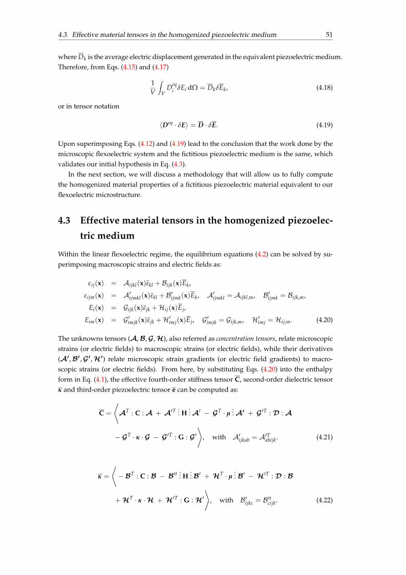
4.3. Effective material tensors in the homogenized piezoelectric medium 51
where Dk is the average electric displacement generated in the equivalent piezoelectric medium.Therefore, from Eqs. (4.15) and (4.17)
1V
Z
VDeq
i dEi dW = DkdEk, (4.18)
or in tensor notation
hDeq · dEi = D · dE. (4.19)
Upon superimposing Eqs. (4.12) and (4.19) lead to the conclusion that the work done by themicroscopic flexoelectric system and the fictitious piezoelectric medium is the same, whichvalidates our initial hypothesis in Eq. (4.3).
In the next section, we will discuss a methodology that will allow us to fully computethe homogenized material properties of a fictitious piezoelectric material equivalent to ourflexoelectric microstructure.
4.3 Effective material tensors in the homogenized piezoelec-tric medium
Within the linear flexoelectric regime, the equilibrium equations (4.2) can be solved by su-perimposing macroscopic strains and electric fields as:
#ij(x) = Aijkl(x)#kl + Bijk(x)Ek,
#ijm(x) = A0ijmkl(x)#kl + B0
ijmk(x)Ek, A0ijmkl = Aijkl,m, B0
ijmk = Bijk,m,
Ei(x) = Gijk(x)#jk +Hij(x)Ej,
Eim(x) = G 0imjk(x)#jk +H0
imj(x)Ej, G 0imjk = Gijk,m, H0
imj = Hij,m. (4.20)
The unknowns tensors (A,B,G,H), also referred as concentration tensors, relate microscopicstrains (or electric fields) to macroscopic strains (or electric fields), while their derivatives(A0,B0,G0,H0) relate microscopic strain gradients (or electric field gradients) to macro-scopic strains (or electric fields). From here, by substituting Eqs. (4.20) into the enthalpyform in Eq. (4.1), the effective fourth-order stiffness tensor C, second-order dielectric tensork and third-order piezoelectric tensor e can be computed as:
C =
*A
T : C : A + A0T ... H
... A0 � GT · µ
... A0 + G0T : D : A
� GT · k · G � G
0T : G : G 0+
, with A0ijkab = A0T
abijk. (4.21)
k =
*�B
T : C : B � B0t ... H
... B0 + HT · µ
... B0 � H0T : D : B
+ HT · k ·H + H
0T : G : H0+
, with B0ijkc = B0t
cijk. (4.22)
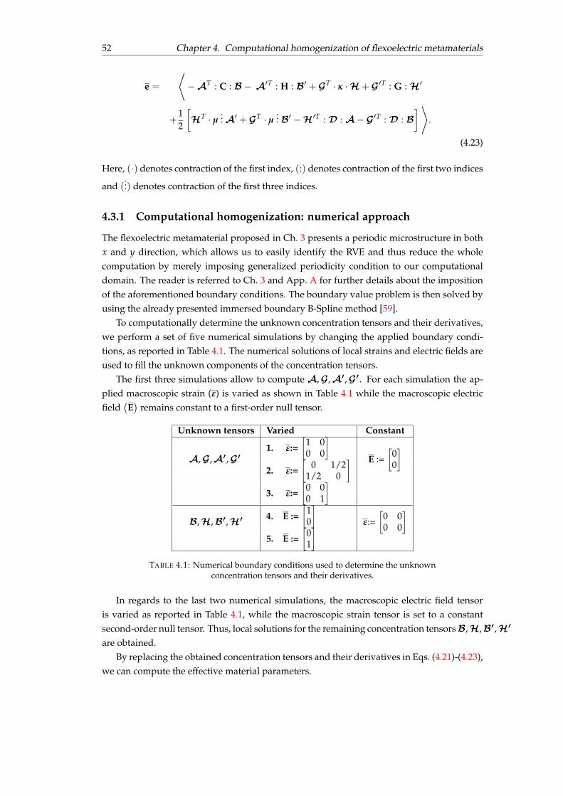
52 Chapter 4. Computational homogenization of flexoelectric metamaterials
e =
*�A
T : C : B� A0T : H : B0 + G
T · k ·H+ G0T : G : H0
+12
H
T · µ... A0 + G
T · µ... B0 �H
0T : D : A� G0T : D : B
�+.
(4.23)
Here, (·) denotes contraction of the first index, (:) denotes contraction of the first two indices
and (...) denotes contraction of the first three indices.
4.3.1 Computational homogenization: numerical approach
The flexoelectric metamaterial proposed in Ch. 3 presents a periodic microstructure in bothx and y direction, which allows us to easily identify the RVE and thus reduce the wholecomputation by merely imposing generalized periodicity condition to our computationaldomain. The reader is referred to Ch. 3 and App. A for further details about the impositionof the aforementioned boundary conditions. The boundary value problem is then solved byusing the already presented immersed boundary B-Spline method [59].
To computationally determine the unknown concentration tensors and their derivatives,we perform a set of five numerical simulations by changing the applied boundary condi-tions, as reported in Table 4.1. The numerical solutions of local strains and electric fields areused to fill the unknown components of the concentration tensors.
The first three simulations allow to compute A,G,A0,G0. For each simulation the ap-plied macroscopic strain (#) is varied as shown in Table 4.1 while the macroscopic electricfield
�E�
remains constant to a first-order null tensor.
Unknown tensors Varied Constant
A,G,A0,G0
1. #:=
1 00 0
�
E :=
00
�
2. #:=
0 1/21/2 0
�
3. #:=
0 00 1
�
B,H,B0,H0 4. E :=
10
�
#:=
0 00 0
�
5. E :=
01
�
TABLE 4.1: Numerical boundary conditions used to determine the unknownconcentration tensors and their derivatives.
In regards to the last two numerical simulations, the macroscopic electric field tensoris varied as reported in Table 4.1, while the macroscopic strain tensor is set to a constantsecond-order null tensor. Thus, local solutions for the remaining concentration tensors B,H,B0,H0
are obtained.By replacing the obtained concentration tensors and their derivatives in Eqs. (4.21)-(4.23),
we can compute the effective material parameters.
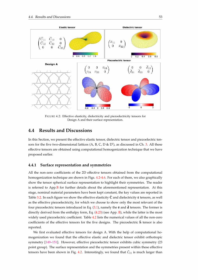
4.4. Results and Discussions 53
FIGURE 4.2: Effective elasticity, dielectricity and piezoelectricity tensors forDesign A and their surface representation.
4.4 Results and Discussions
In this Section, we present the effective elastic tensor, dielectric tensor and piezoelectric ten-sors for the five two-dimensional lattices (A, B, C, D & D0), as discussed in Ch. 3. All theseeffective tensors are obtained using computational homogenization technique that we haveproposed earlier.
4.4.1 Surface representation and symmetries
All the non-zero coefficients of the 2D effective tensors obtained from the computationalhomogenization technique are shown in Figs. 4.2-4.6. For each of them, we also graphicallyshow the tensor spherical surface representation to highlight their symmetries. The readeris referred to App.B for further details about the aforementioned representation. At thisstage, nominal material parameters have been kept constant, the key values are reported inTable 3.2. In each figure we show the effective elasticity C and dielectricity k tensors, as wellas the effective piezoelectricity, for which we choose to show only the most relevant of thefour piezoelectric tensors introduced in Eq. (3.1), namely the e and d tensors. The former isdirectly derived from the enthalpy form, Eq. (4.23) (see App. B), while the latter is the mostwidely used piezoelectric coefficient. Table 4.2 lists the numerical values of all the non-zerocoefficients of the effective tensors for the five designs. The piezoelectric h tensor is alsoreported.
We first evaluated effective tensors for design A. With the help of computational ho-mogenization we found that the effective elastic and dielectric tensor exhibit orthotropicsymmetry [149–151]. However, effective piezoelectric tensor exhibits cubic symmetry (23point group). The surface representation and the symmetries present within these effectivetensors have been shown in Fig. 4.2. Interestingly, we found that C11 is much larger than

54 Chapter 4. Computational homogenization of flexoelectric metamaterials
FIGURE 4.3: Effective elasticity, dielectricity and piezoelectricity tensors forDesign B and their surface representation.
C22, cf. Table 4.2, which implies that the material provides more resistance to the deforma-tion in y-direction. Similarly, we found that k11 is greater than k22. However, in the case ofthe effective piezoelectric stress-charge tensor e [152], the transverse shear mode component(e13) is largest in magnitude when compared with longitudinal and transverse coefficients.A similar trend is observed in the effective piezoelectric strain-charge d and h tensors. Thisbehavior, similar to that of strong piezoelectrics such as PZT, which also exhibits largestshear piezoelectricity, implies that our proposed design A generates large polarization whensubjected to shear strain and thus can be effectively used as a shear-based energy harvester[153–155]. It is indeed well known that in energy harvesting, the operation mode stronglyaffects the quantification of the electromechanical coupling coefficient, evaluated as a measureof the capability of the device to convert the input mechanical energy into electrical energy.For design B and design C we found that the effective elastic tensor has square (tetragonal)symmetry. However, the effective dielectric tensor behaves isotropically while the effectivepiezoelectric tensors, which present three coefficients having the same magnitude, exhibitrectangular symmetry. Since our piezoelectric coefficients are same in all the directions, thedevice can be readily used for either transverse shear, transverse or longitudinal operationmode, indifferently. Based on the magnitudes we also found out that design B works betterthan design C in both actuator mode (d) as well as sensor mode (h) when displacementsand electric potential are measured respectively. On the contrary, design C performs betterin actuator mode (e) when stresses/forces are measured. Fig. 4.3 and 4.4 represent the sur-faces for these effective tensors for design B and C respectively. Finally, we studied the mostperformant designs D and D0. As anticipated by the lack of symmetry in the geometries,we noticed that both design D and D0 are fully anisotropic. The designs and their surfacerepresentation can be seen from Fig. 4.5 and 4.6. In general, we noticed that both designsare significantly more compliant than the others, which partially explains the better perfo-mance. For design D, we further notice that the sensor performs better in transverse shear
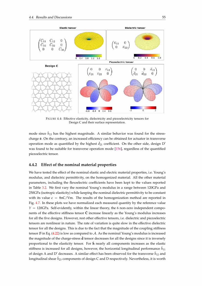
4.4. Results and Discussions 55
FIGURE 4.4: Effective elasticity, dielectricity and piezoelectricity tensors forDesign C and their surface representation.
mode since h13 has the highest magnitude. A similar behavior was found for the stress-charge e. On the contrary, an increased efficiency can be obtained for actuator in transverseoperation mode as quantified by the highest d21 coefficient. On the other side, design D0
was found to be suitable for transverse operation mode [156], regardless of the quantifiedpiezoelectric tensor.
4.4.2 Effect of the nominal material properties
We have tested the effect of the nominal elastic and electric material properties, i.e. Young’smodulus, and dielectric permittivity, on the homogenized material. All the other materialparameters, including the flexoelectric coefficients have been kept to the values reportedin Table 3.2. We first vary the nominal Young’s modulus in a range between 120GPa and250GPa (isotropic elasticity) while keeping the nominal dielectric permittivity to be constantwith its value e = 8nC/Vm. The results of the homogenization method are reported inFig. 4.7. In these plots we have normalized each measured quantity by the reference valueY = 120GPa. Self-evidently, within the linear theory, the 6 non-zero independent compo-nents of the effective stiffness tensor C increase linearly as the Young’s modulus increasesfor all the five designs. However, rest other effective tensors, i.e. dielectric and piezoelectrictensors are nonlinear in nature. The rate of variation is quite slow in the effective dielectrictensor for all the designs. This is due to the fact that the magnitude of the coupling stiffnesstensor B in Eq. (4.22) is low as compared to A. As the nominal Young’s modulus is increasedthe magnitude of the charge-stress d tensor decreases for all the designs since it is inverselyproportional to the elasticity tensor. For h nearly all components increases as the elasticstiffness is increased for all designs, however, the horizontal longitudinal performance h11
of design A and D0 decreases. A similar effect has been observed for the transverse h12 andlongitudinal shear h23 components of design C and D respectively. Nevertheless, it is worth
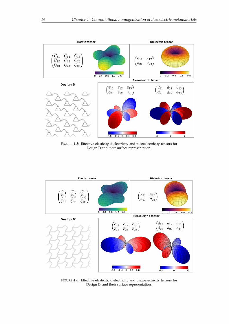
56 Chapter 4. Computational homogenization of flexoelectric metamaterials
FIGURE 4.5: Effective elasticity, dielectricity and piezoelectricity tensors forDesign D and their surface representation.
FIGURE 4.6: Effective elasticity, dielectricity and piezoelectricity tensors forDesign D’ and their surface representation.
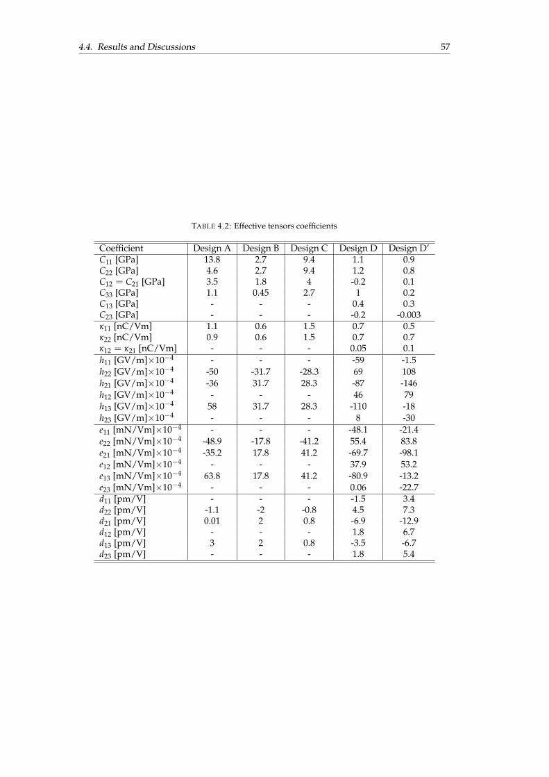
4.4. Results and Discussions 57
TABLE 4.2: Effective tensors coefficients
Coefficient Design A Design B Design C Design D Design D’C11 [GPa] 13.8 2.7 9.4 1.1 0.9C22 [GPa] 4.6 2.7 9.4 1.2 0.8C12 = C21 [GPa] 3.5 1.8 4 -0.2 0.1C33 [GPa] 1.1 0.45 2.7 1 0.2C13 [GPa] - - - 0.4 0.3C23 [GPa] - - - -0.2 -0.003k11 [nC/Vm] 1.1 0.6 1.5 0.7 0.5k22 [nC/Vm] 0.9 0.6 1.5 0.7 0.7k12 = k21 [nC/Vm] - - - 0.05 0.1h11 [GV/m]⇥10�4 - - - -59 -1.5h22 [GV/m]⇥10�4 -50 -31.7 -28.3 69 108h21 [GV/m]⇥10�4 -36 31.7 28.3 -87 -146h12 [GV/m]⇥10�4 - - - 46 79h13 [GV/m]⇥10�4 58 31.7 28.3 -110 -18h23 [GV/m]⇥10�4 - - - 8 -30e11 [mN/Vm]⇥10�4 - - - -48.1 -21.4e22 [mN/Vm]⇥10�4 -48.9 -17.8 -41.2 55.4 83.8e21 [mN/Vm]⇥10�4 -35.2 17.8 41.2 -69.7 -98.1e12 [mN/Vm]⇥10�4 - - - 37.9 53.2e13 [mN/Vm]⇥10�4 63.8 17.8 41.2 -80.9 -13.2e23 [mN/Vm]⇥10�4 - - - 0.06 -22.7d11 [pm/V] - - - -1.5 3.4d22 [pm/V] -1.1 -2 -0.8 4.5 7.3d21 [pm/V] 0.01 2 0.8 -6.9 -12.9d12 [pm/V] - - - 1.8 6.7d13 [pm/V] 3 2 0.8 -3.5 -6.7d23 [pm/V] - - - 1.8 5.4
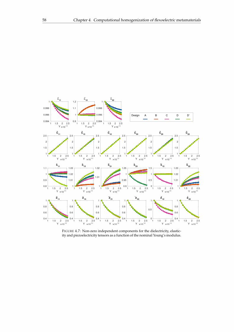
58 Chapter 4. Computational homogenization of flexoelectric metamaterials
Design C DBA D'
1 1.5 2 2.5Y ×10 11
0.994
0.996
0.998
1
1 1.5 2 2.5Y ×10 11
0.9
1
1.1
1.2
1 1.5 2 2.5Y ×10 11
0.994
0.996
0.998
1
1 1.5 2 2.5Y ×10 11
1
1.5
2
2.5
1 1.5 2 2.5Y ×10 11
1
1.5
2
2.5
1 1.5 2 2.5Y ×10 11
1
1.5
2
2.5
1 1.5 2 2.5Y ×10 11
1
1.5
2
2.5
1 1.5 2 2.5Y ×10 11
1
1.5
2
2.5
1 1.5 2 2.5Y ×10 11
1
1.5
2
2.5
1 1.5 2 2.5Y ×10 11
0.8
0.9
1
1.1
1 1.5 2 2.5Y ×10 11
1
1.01
1.02
1.03
1 1.5 2 2.5Y ×10 11
1
1.01
1.02
1 1.5 2 2.5Y ×10 11
0.9
0.95
1
1.05
1 1.5 2 2.5Y ×10 11
0
0.5
1
1.5
1 1.5 2 2.5Y ×10 11
1
1.01
1.02
1.03
1 1.5 2 2.5Y ×10 11
0.4
0.6
0.8
1
1 1.5 2 2.5Y ×10 11
0.4
0.6
0.8
1
1 1.5 2 2.5Y ×10 11
0.4
0.6
0.8
1
1 1.5 2 2.5Y ×10 11
0.4
0.6
0.8
1
1 1.5 2 2.5Y ×10 11
0
0.5
1
1 1.5 2 2.5Y ×10 11
0.4
0.6
0.8
1
�11 �12 �22
C11 C13 C12 C33 C23 C22
h11 h13 h21 h23 h12 h22
d 11 d 13 d 21 d 23 d 12 d 22
FIGURE 4.7: Non-zero independent components for the dielectricity, elastic-ity and piezoelectricity tensors as a function of the nominal Young’s modulus.
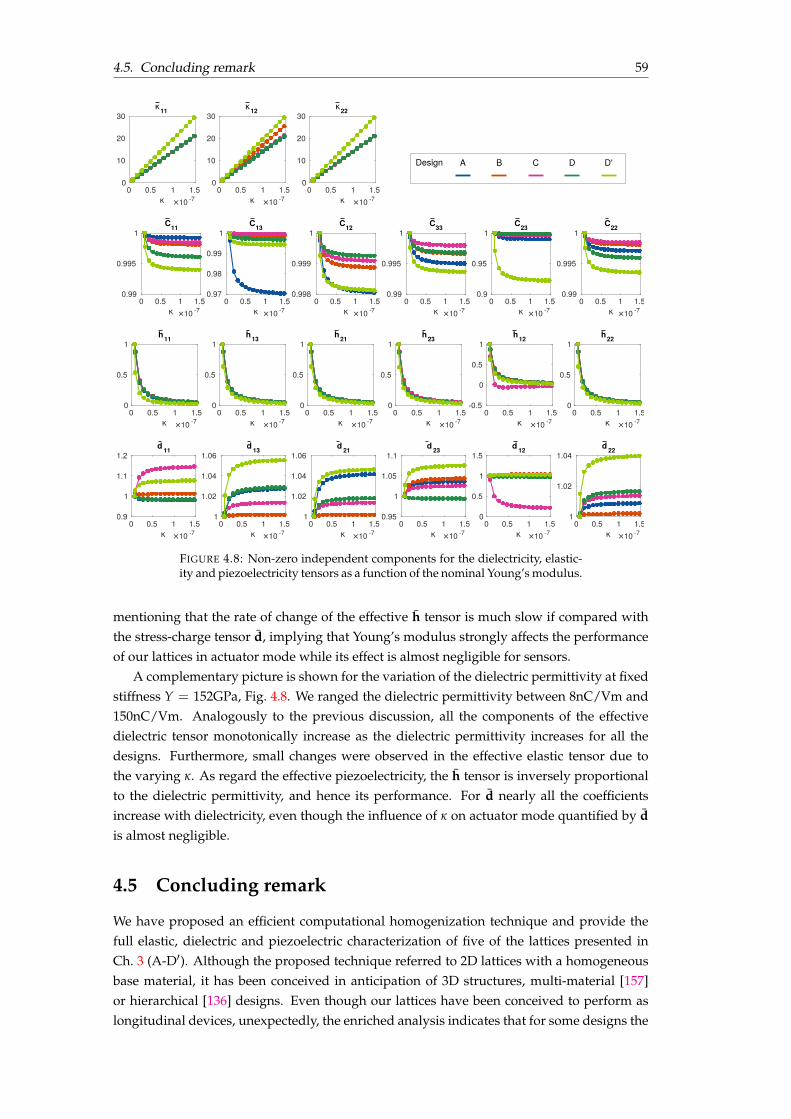
4.5. Concluding remark 59
Design C DBA D'
0 0.5 1 1.5� ×10 -7
0
10
20
30�11
0 0.5 1 1.5� ×10 -7
0
10
20
30�12
0 0.5 1 1.5� ×10 -7
0
10
20
30�22
0 0.5 1 1.5� ×10 -7
0.99
0.995
1C11
0 0.5 1 1.5� ×10 -7
0.97
0.98
0.99
1C13
0 0.5 1 1.5� ×10 -7
0.998
0.999
1C12
0 0.5 1 1.5� ×10 -7
0.99
0.995
1C33
0 0.5 1 1.5� ×10 -7
0.9
0.95
1C23
0 0.5 1 1.5� ×10 -7
0.99
0.995
1C22
0 0.5 1 1.5� ×10 -7
0
0.5
1h11
0 0.5 1 1.5� ×10 -7
0
0.5
1h13
0 0.5 1 1.5� ×10 -7
0
0.5
1h21
0 0.5 1 1.5� ×10 -7
0
0.5
1h23
0 0.5 1 1.5� ×10 -7
-0.5
0
0.5
1h12
0 0.5 1 1.5� ×10 -7
0
0.5
1h22
0 0.5 1 1.5� ×10 -7
0.9
1
1.1
1.2d 11
0 0.5 1 1.5� ×10 -7
1
1.02
1.04
1.06d 13
0 0.5 1 1.5� ×10 -7
1
1.02
1.04
1.06d 21
0 0.5 1 1.5� ×10 -7
0.95
1
1.05
1.1d 23
0 0.5 1 1.5� ×10 -7
0
0.5
1
1.5d 12
0 0.5 1 1.5� ×10 -7
1
1.02
1.04d 22
FIGURE 4.8: Non-zero independent components for the dielectricity, elastic-ity and piezoelectricity tensors as a function of the nominal Young’s modulus.
mentioning that the rate of change of the effective h tensor is much slow if compared withthe stress-charge tensor d, implying that Young’s modulus strongly affects the performanceof our lattices in actuator mode while its effect is almost negligible for sensors.
A complementary picture is shown for the variation of the dielectric permittivity at fixedstiffness Y = 152GPa, Fig. 4.8. We ranged the dielectric permittivity between 8nC/Vm and150nC/Vm. Analogously to the previous discussion, all the components of the effectivedielectric tensor monotonically increase as the dielectric permittivity increases for all thedesigns. Furthermore, small changes were observed in the effective elastic tensor due tothe varying k. As regard the effective piezoelectricity, the h tensor is inversely proportionalto the dielectric permittivity, and hence its performance. For d nearly all the coefficientsincrease with dielectricity, even though the influence of k on actuator mode quantified by dis almost negligible.
4.5 Concluding remark
We have proposed an efficient computational homogenization technique and provide thefull elastic, dielectric and piezoelectric characterization of five of the lattices presented inCh. 3 (A-D0). Although the proposed technique referred to 2D lattices with a homogeneousbase material, it has been conceived in anticipation of 3D structures, multi-material [157]or hierarchical [136] designs. Even though our lattices have been conceived to perform aslongitudinal devices, unexpectedly, the enriched analysis indicates that for some designs the

60 Chapter 4. Computational homogenization of flexoelectric metamaterials
larger effective piezoelectric coefficient is not the longitudinal one, but instead the shear orthe transverse, hence, suggesting the preferred operation mode of each of our lattices for theeffective piezoelectric tensor of interest. According to our previous intuition designs B andC exhibit a larger longitudinal piezoelectric coefficient, and can thus be identified as suitablefor longitudinal sensors or actuators. On the contrary, design A, D and D0 manifest a largertransverse shear and transverse coefficient with respect to the longitudinal evaluated alongthe loading direction.

61
Chapter 5
On-going work
In Chapter 3 we have introduced a class of 2D low-area fraction lattices, analyzed the effectof lattice geometry, orientation and area fraction and proved that even without attemptinga methodical optimization of the geometries we were able to considerably improve the per-formance of our lattices. In Chapter 4 we have quantified the full piezoelectric tensor andgained insights on the overall behavior of our lattices. Design D0 has proven itself to be themost effective design, in different operation modes.
In this chapter we will present a preliminary systematic shape-parameters optimizationstudy of the 2D bending-dominated lattices in order to seek the optimal shape for a giventopological configuration. Finally, we will perform a more general optimization analysisincluding the effect of the nominal material properties on the performance of our lattice.
5.1 Optimization methods
The numerical optimization has been performed by merging the already existing MatLaboptimization toolbox with our immersed boundary B-spline framework. We employed dif-ferent optimization algorithms all of them apt for constrained and unconstrained problems.The methods can be classified in two main subcategories, namely gradient-based and stochas-tic. In the following, we will briefly discuss their leading features.
5.1.1 Gradient-based methods
All gradient-based algorithms for optimization have some common features. In generalthese methods, as suggested by their name, at each step evaluate gradients to identify thesearch direction for the next point. As a consequence, all the functions that define the prob-lem (i.e. objective and restriction functions), as well as the design variables are assumed tobe continuous within the feasible design space.
The optimization problem is mathematically stated as
minx1,...,n
f (x) such that
8>>>>>><
>>>>>>:
Ax b,A = [A1
x1, ..., A1
xn ; ...; ANx1
, ..., ANxn ],
b = [b1, ..., bN ]T ;
c(x) 0, non-linear constraints;
lb x ub, lower and upper bound for the solution.
(5.1)
where f (x) is the continuous and differentiable objective function, with x = [x1, ..., xn]T beinga n�vector representing the minimizers, also called design variables, for the objective functionunder consideration. The general structure of all gradient-based methods is described in the
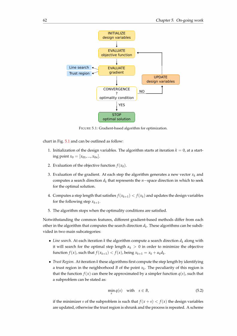
62 Chapter 5. On-going work
INITIALIZE design variables
CONVERGENCE?
optimality condition
EVALUATE gradient
EVALUATE objective function
UPDATEdesign variables
STOPoptimal solution
YES
NO
Trust regionLine search
FIGURE 5.1: Gradient-based algorithm for optimization.
chart in Fig. 5.1 and can be outlined as follow:
1. Initialization of the design variables. The algorithm starts at iteration k = 0, at a start-ing point x0 = [x01, ..., x0n].
2. Evaluation of the objective function f (x0).
3. Evaluation of the gradient. At each step the algorithm generates a new vector xk andcomputes a search direction dk that represents the n�space direction in which to seekfor the optimal solution.
4. Computes a step length that satisfies f (xk+1) < f (xk) and updates the design variablesfor the following step xk+1.
5. The algorithm stops when the optimality conditions are satisfied.
Notwithstanding the common features, different gradient-based methods differ from eachother in the algorithm that computes the search direction dk. These algorithms can be subdi-vided in two main subcategories:
• Line search. At each iteration k the algorithm compute a search direction dk along withit will search for the optimal step length ak > 0 in order to minimize the objectivefunction f (x), such that f (xk+1) < f (x), being xk+1 = xk + akdk.
• Trust Region. At iteration k these algorithms first compute the step length by identifyinga trust region in the neighborhood B of the point xk. The peculiarity of this region isthat the function f (x) can there be approximated by a simpler function q(s), such thata subproblem can be stated as:
mins
q(s) with s 2 B, (5.2)
if the minimizer s of the subproblem is such that f (x + s) < f (x) the design variablesare updated, otherwise the trust region is shrunk and the process is repeated. A scheme
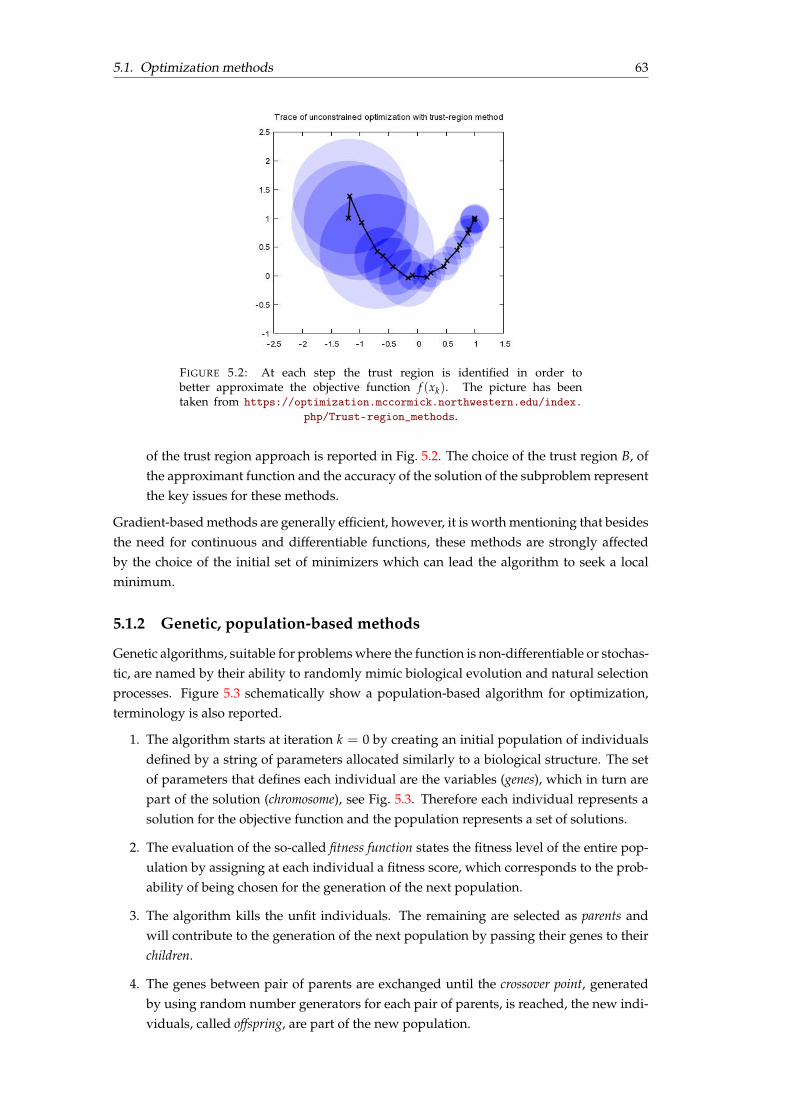
5.1. Optimization methods 63
FIGURE 5.2: At each step the trust region is identified in order tobetter approximate the objective function f (xk). The picture has beentaken from https://optimization.mccormick.northwestern.edu/index.
php/Trust-region_methods.
of the trust region approach is reported in Fig. 5.2. The choice of the trust region B, ofthe approximant function and the accuracy of the solution of the subproblem representthe key issues for these methods.
Gradient-based methods are generally efficient, however, it is worth mentioning that besidesthe need for continuous and differentiable functions, these methods are strongly affectedby the choice of the initial set of minimizers which can lead the algorithm to seek a localminimum.
5.1.2 Genetic, population-based methods
Genetic algorithms, suitable for problems where the function is non-differentiable or stochas-tic, are named by their ability to randomly mimic biological evolution and natural selectionprocesses. Figure 5.3 schematically show a population-based algorithm for optimization,terminology is also reported.
1. The algorithm starts at iteration k = 0 by creating an initial population of individualsdefined by a string of parameters allocated similarly to a biological structure. The setof parameters that defines each individual are the variables (genes), which in turn arepart of the solution (chromosome), see Fig. 5.3. Therefore each individual represents asolution for the objective function and the population represents a set of solutions.
2. The evaluation of the so-called fitness function states the fitness level of the entire pop-ulation by assigning at each individual a fitness score, which corresponds to the prob-ability of being chosen for the generation of the next population.
3. The algorithm kills the unfit individuals. The remaining are selected as parents andwill contribute to the generation of the next population by passing their genes to theirchildren.
4. The genes between pair of parents are exchanged until the crossover point, generatedby using random number generators for each pair of parents, is reached, the new indi-viduals, called offspring, are part of the new population.
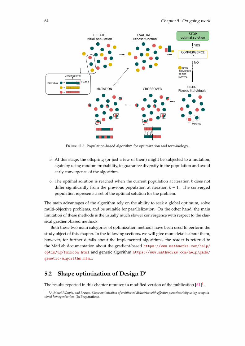
64 Chapter 5. On-going work
CREATEInitial population
EVALUATEFitness function
CONVERGENCE?
STOPoptimal solution
YES
NO
SELECTFitness individualsCROSSOVERMUTATION
un�t individuals do not survive
Individual = Gene
Chromosome
==
Parents
FIGURE 5.3: Population-based algorithm for optimization and terminology.
5. At this stage, the offspring (or just a few of them) might be subjected to a mutation,again by using random probability, to guarantee diversity in the population and avoidearly convergence of the algorithm.
6. The optimal solution is reached when the current population at iteration k does notdiffer significantly from the previous population at iteration k � 1. The convergedpopulation represents a set of the optimal solution for the problem.
The main advantages of the algorithm rely on the ability to seek a global optimum, solvemulti-objective problems, and be suitable for parallelization. On the other hand, the mainlimitation of these methods is the usually much slower convergence with respect to the clas-sical gradient-based methods.
Both these two main categories of optimization methods have been used to perform thestudy object of this chapter. In the following sections, we will give more details about them,however, for further details about the implemented algorithms, the reader is referred tothe MatLab documentation about the gradient-based https://www.mathworks.com/help/optim/ug/fmincon.html and genetic algorithm https://www.mathworks.com/help/gads/genetic-algorithm.html.
5.2 Shape optimization of Design D0
The results reported in this chapter represent a modified version of the publication [61]1.1A.Mocci,P.Gupta, and I.Arias. Shape optimization of architected dielectrics with effective piezoelectricity using computa-
tional homogenization. (In Preparation).
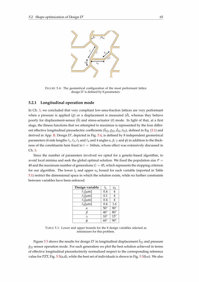
5.2. Shape optimization of Design D0 65
FIGURE 5.4: The geometrical configuration of the most performant latticedesign D’ is defined by 8 parameters.
5.2.1 Longitudinal operation mode
In Ch. 3, we concluded that very compliant low-area-fraction lattices are very performantwhen a pressure is applied (g) or a displacement is measured (d), whereas they behavepoorly for displacement-sensor (h) and stress-actuator (e) mode. In light of that, at a firststage, the fitness functions that we attempted to maximize is represented by the four differ-ent effective longitudinal piezoelectric coefficients (h22, g22, d22, e22), defined in Eq. (3.1) andderived in App. B. Design D0, depicted in Fig. 5.4, is defined by 8 independent geometricalparameters (4 side lengths `1, `2, `3 and `4 and 4 angles a, b, g and f) in addition to the thick-ness of the constituents here fixed to t = 160nm, whose effect was extensively discussed inCh. 3.
Since the number of parameters involved we opted for a genetic-based algorithm, toavoid local minima and seek the global optimal solution. We fixed the population size P =
48 and the maximum number of generations G = 45, which represents the stopping criterionfor our algorithm. The lower lb and upper ub bound for each variable (reported in Table5.1) restrict the dimensional space in which the solution exists, while no further constraintsbetween variables have been enforced.
Design variable lb ub`1[µm] 0.4 4`2[µm] 0.1 4`3[µm] 0.4 4`4[µm] 0.4 1.6
a 50� 90�b 40� 80�g 10� 15�f 60� 90�
TABLE 5.1: Lower and upper bounds for the 8 design variables selected asminimizers for this problem.
Figure 5.5 shows the results for design D0 in longitudinal displacement h22 and pressureg22 sensor operation mode. For each generation we plot the best solution achieved in termsof effective longitudinal piezoelectricity normalized respect to the corresponding referencevalue for PZT, Fig. 5.5(a,d), while the best set of individuals is shown in Fig. 5.5(b,e). We also
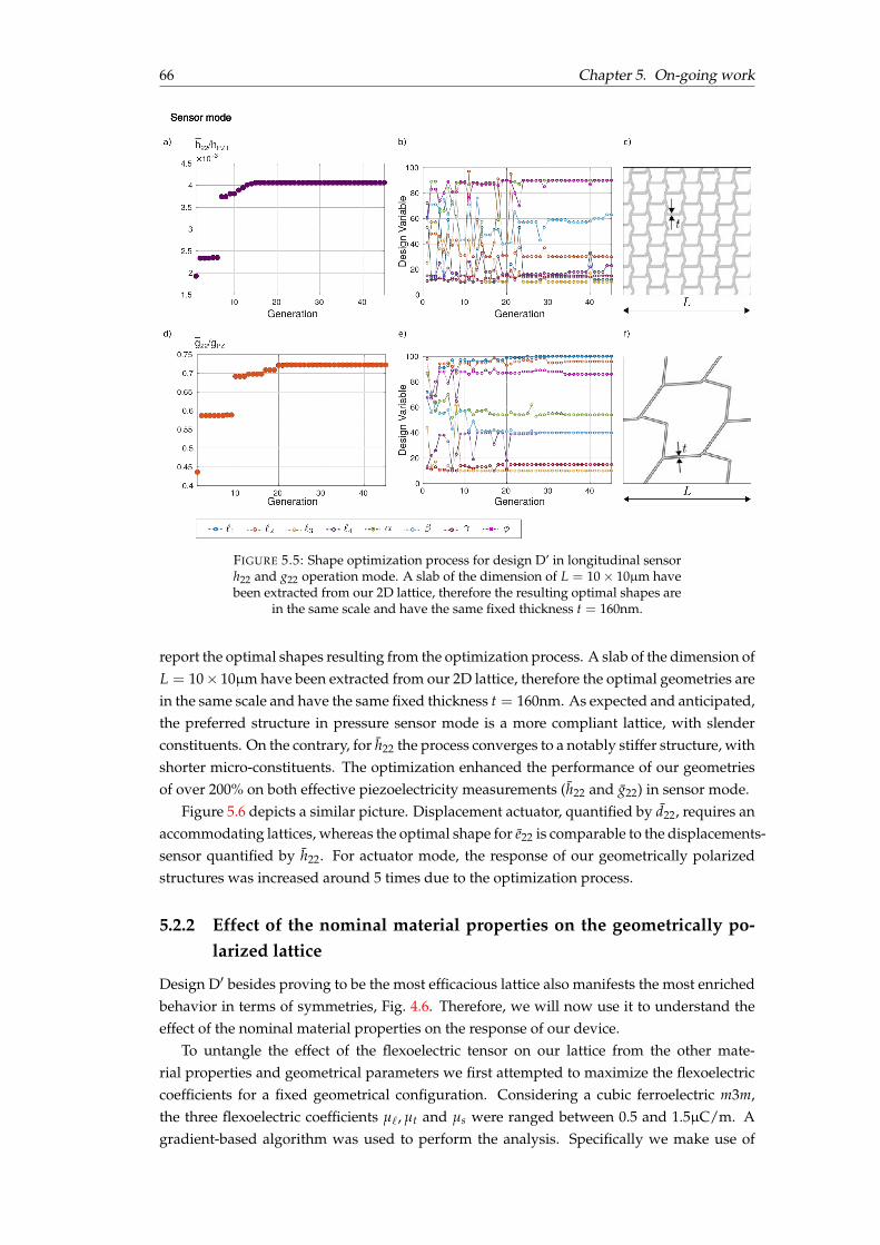
66 Chapter 5. On-going work
FIGURE 5.5: Shape optimization process for design D’ in longitudinal sensorh22 and g22 operation mode. A slab of the dimension of L = 10 ⇥ 10µm havebeen extracted from our 2D lattice, therefore the resulting optimal shapes are
in the same scale and have the same fixed thickness t = 160nm.
report the optimal shapes resulting from the optimization process. A slab of the dimension ofL = 10⇥ 10µm have been extracted from our 2D lattice, therefore the optimal geometries arein the same scale and have the same fixed thickness t = 160nm. As expected and anticipated,the preferred structure in pressure sensor mode is a more compliant lattice, with slenderconstituents. On the contrary, for h22 the process converges to a notably stiffer structure, withshorter micro-constituents. The optimization enhanced the performance of our geometriesof over 200% on both effective piezoelectricity measurements (h22 and g22) in sensor mode.
Figure 5.6 depicts a similar picture. Displacement actuator, quantified by d22, requires anaccommodating lattices, whereas the optimal shape for e22 is comparable to the displacements-sensor quantified by h22. For actuator mode, the response of our geometrically polarizedstructures was increased around 5 times due to the optimization process.
5.2.2 Effect of the nominal material properties on the geometrically po-larized lattice
Design D0 besides proving to be the most efficacious lattice also manifests the most enrichedbehavior in terms of symmetries, Fig. 4.6. Therefore, we will now use it to understand theeffect of the nominal material properties on the response of our device.
To untangle the effect of the flexoelectric tensor on our lattice from the other mate-rial properties and geometrical parameters we first attempted to maximize the flexoelectriccoefficients for a fixed geometrical configuration. Considering a cubic ferroelectric m3m,the three flexoelectric coefficients µ`, µt and µs were ranged between 0.5 and 1.5µC/m. Agradient-based algorithm was used to perform the analysis. Specifically we make use of
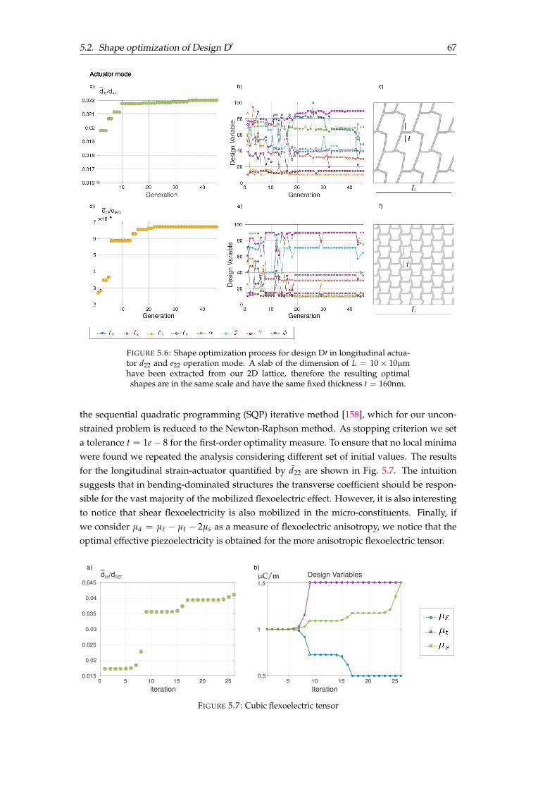
5.2. Shape optimization of Design D0 67
FIGURE 5.6: Shape optimization process for design D0 in longitudinal actua-tor d22 and e22 operation mode. A slab of the dimension of L = 10 ⇥ 10µmhave been extracted from our 2D lattice, therefore the resulting optimalshapes are in the same scale and have the same fixed thickness t = 160nm.
the sequential quadratic programming (SQP) iterative method [158], which for our uncon-strained problem is reduced to the Newton-Raphson method. As stopping criterion we seta tolerance t = 1e � 8 for the first-order optimality measure. To ensure that no local minimawere found we repeated the analysis considering different set of initial values. The resultsfor the longitudinal strain-actuator quantified by d22 are shown in Fig. 5.7. The intuitionsuggests that in bending-dominated structures the transverse coefficient should be respon-sible for the vast majority of the mobilized flexoelectric effect. However, it is also interestingto notice that shear flexoelectricity is also mobilized in the micro-constituents. Finally, ifwe consider µa = µ` � µt � 2µs as a measure of flexoelectric anisotropy, we notice that theoptimal effective piezoelectricity is obtained for the more anisotropic flexoelectric tensor.
iteration5 10 15 20 25
0.5
1.5Design Variables
Iteration
d22/dPZT
a) b)
0 5 10 15 20 250.015
0.02
0.025
0.03
0.035
0.04
0.045
1
FIGURE 5.7: Cubic flexoelectric tensor
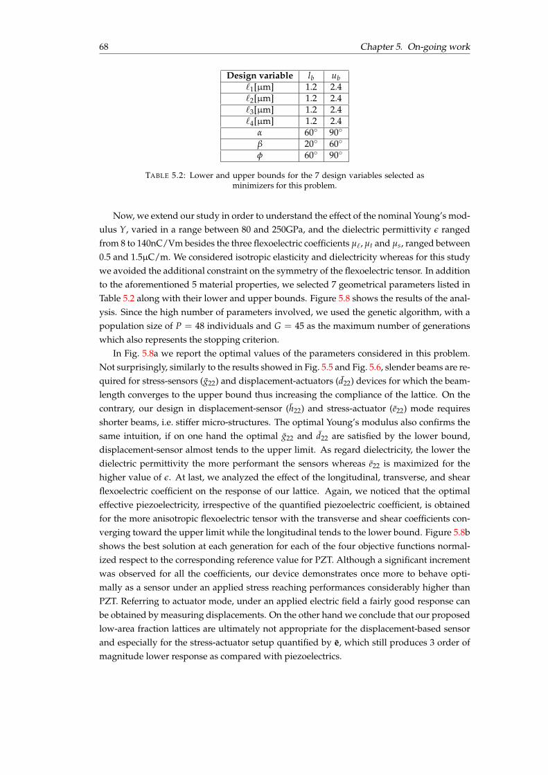
68 Chapter 5. On-going work
Design variable lb ub`1[µm] 1.2 2.4`2[µm] 1.2 2.4`3[µm] 1.2 2.4`4[µm] 1.2 2.4
a 60� 90�b 20� 60�f 60� 90�
TABLE 5.2: Lower and upper bounds for the 7 design variables selected asminimizers for this problem.
Now, we extend our study in order to understand the effect of the nominal Young’s mod-ulus Y, varied in a range between 80 and 250GPa, and the dielectric permittivity e rangedfrom 8 to 140nC/Vm besides the three flexoelectric coefficients µ`, µt and µs, ranged between0.5 and 1.5µC/m. We considered isotropic elasticity and dielectricity whereas for this studywe avoided the additional constraint on the symmetry of the flexoelectric tensor. In additionto the aforementioned 5 material properties, we selected 7 geometrical parameters listed inTable 5.2 along with their lower and upper bounds. Figure 5.8 shows the results of the anal-ysis. Since the high number of parameters involved, we used the genetic algorithm, with apopulation size of P = 48 individuals and G = 45 as the maximum number of generationswhich also represents the stopping criterion.
In Fig. 5.8a we report the optimal values of the parameters considered in this problem.Not surprisingly, similarly to the results showed in Fig. 5.5 and Fig. 5.6, slender beams are re-quired for stress-sensors (g22) and displacement-actuators (d22) devices for which the beam-length converges to the upper bound thus increasing the compliance of the lattice. On thecontrary, our design in displacement-sensor (h22) and stress-actuator (e22) mode requiresshorter beams, i.e. stiffer micro-structures. The optimal Young’s modulus also confirms thesame intuition, if on one hand the optimal g22 and d22 are satisfied by the lower bound,displacement-sensor almost tends to the upper limit. As regard dielectricity, the lower thedielectric permittivity the more performant the sensors whereas e22 is maximized for thehigher value of e. At last, we analyzed the effect of the longitudinal, transverse, and shearflexoelectric coefficient on the response of our lattice. Again, we noticed that the optimaleffective piezoelectricity, irrespective of the quantified piezoelectric coefficient, is obtainedfor the more anisotropic flexoelectric tensor with the transverse and shear coefficients con-verging toward the upper limit while the longitudinal tends to the lower bound. Figure 5.8bshows the best solution at each generation for each of the four objective functions normal-ized respect to the corresponding reference value for PZT. Although a significant incrementwas observed for all the coefficients, our device demonstrates once more to behave opti-mally as a sensor under an applied stress reaching performances considerably higher thanPZT. Referring to actuator mode, under an applied electric field a fairly good response canbe obtained by measuring displacements. On the other hand we conclude that our proposedlow-area fraction lattices are ultimately not appropriate for the displacement-based sensorand especially for the stress-actuator setup quantified by e, which still produces 3 order ofmagnitude lower response as compared with piezoelectrics.
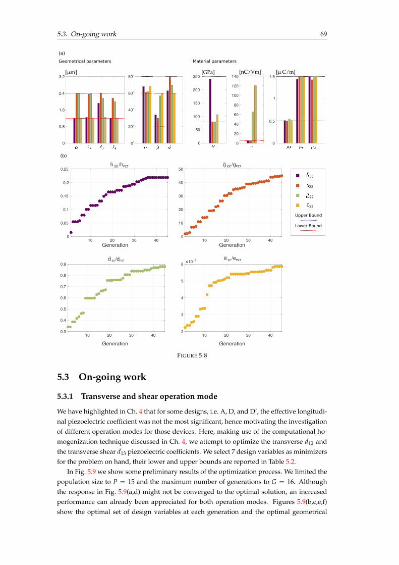
5.3. On-going work 69
10 20 30 400
0.05
0.1
0.15
0.2
0.25
Upper Bound
Lower Bound
Generation Generation
Generation Generation
Material parametersGeometrical parameters
22
22
22
22
(a)
(b)
0
0.8
1.6
2.4
3.2
0
20
40
60
80
0
50
100
150
200
250
0
0.5
1
1.5140
120
100
80
60
40
20
0
h 22 /hPZT g 22 /gPZT
d 22 /dPZT e 22 /ePZT
10 20 30 400.3
0.4
0.5
0.6
0.7
0.8
0.9
10 20 30 402
3
4
5
6 ×10 -3
10 20 30 400
10
20
30
40
50
FIGURE 5.8
5.3 On-going work
5.3.1 Transverse and shear operation mode
We have highlighted in Ch. 4 that for some designs, i.e. A, D, and D’, the effective longitudi-nal piezoelectric coefficient was not the most significant, hence motivating the investigationof different operation modes for those devices. Here, making use of the computational ho-mogenization technique discussed in Ch. 4, we attempt to optimize the transverse d12 andthe transverse shear d13 piezoelectric coefficients. We select 7 design variables as minimizersfor the problem on hand, their lower and upper bounds are reported in Table 5.2.
In Fig. 5.9 we show some preliminary results of the optimization process. We limited thepopulation size to P = 15 and the maximum number of generations to G = 16. Althoughthe response in Fig. 5.9(a,d) might not be converged to the optimal solution, an increasedperformance can already been appreciated for both operation modes. Figures 5.9(b,c,e,f)show the optimal set of design variables at each generation and the optimal geometrical
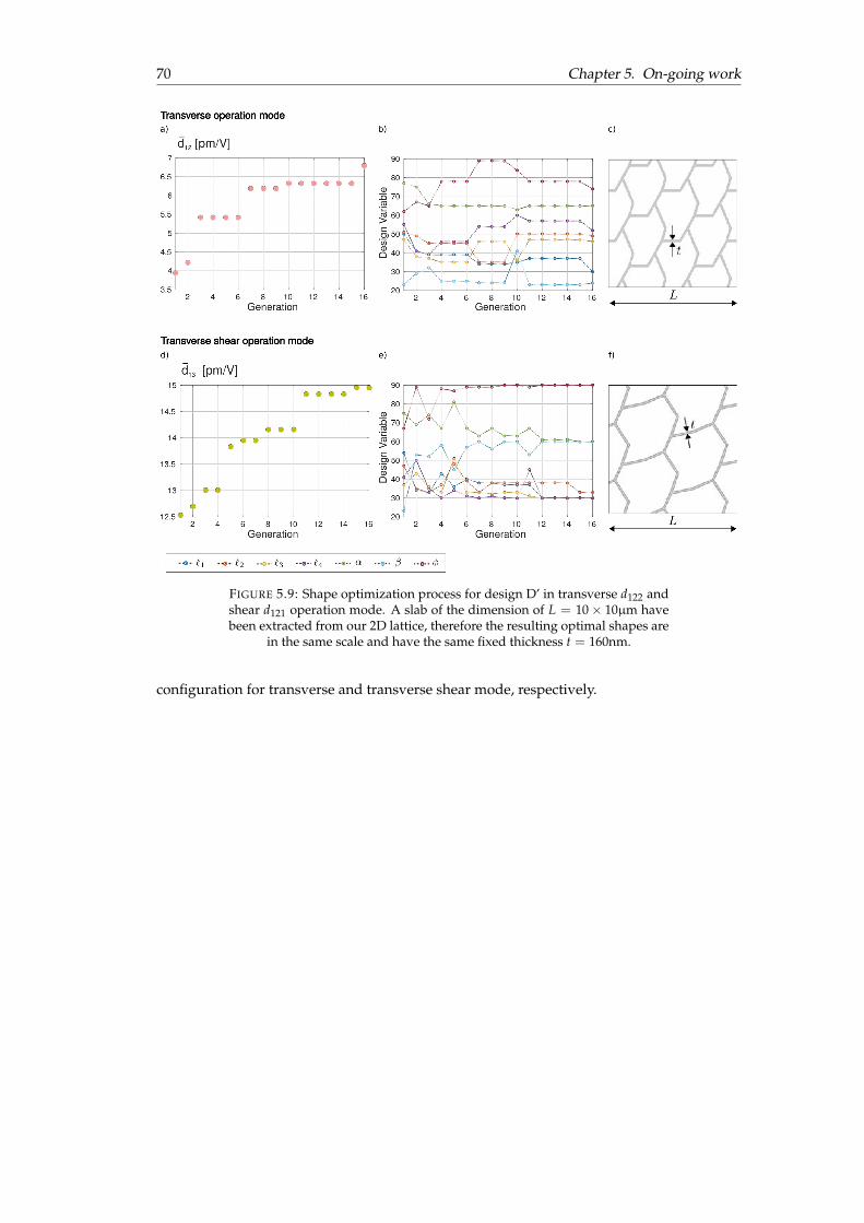
70 Chapter 5. On-going work
FIGURE 5.9: Shape optimization process for design D’ in transverse d122 andshear d121 operation mode. A slab of the dimension of L = 10 ⇥ 10µm havebeen extracted from our 2D lattice, therefore the resulting optimal shapes are
in the same scale and have the same fixed thickness t = 160nm.
configuration for transverse and transverse shear mode, respectively.
71
Chapter 6
Towards 3D flexoelectricmetamaterials and devices:flexoelectricity under torsion
In the first part of this manuscript, we focused our attention on the identification of two-dimensional setups with the aim of identifying suitable building blocks for geometricallypolarized metamaterials. At this stage, further investigations will be oriented toward thedetection of 3D building blocks for metamaterials to enhance the performance of our lattices.
Three-dimensional setups also enable more complex ways of mobilizing gradients, be-sides bending and compression of non-uniform geometries, torsion is indeed another clas-sical method to induce strong strain gradients [159–161]. Notwithstanding torsion of thinrods has been extensively used to characterize strain-gradient elasticity [162] and plasticity[159, 161] yet surprisingly flexoelectricity has been barely studied in this setting [163, 164]and in particular, to the best of our knowledge there are no studies on torsion of cubic per-ovskites, which are the strongest flexoelectrics among all dielectrics [27]. The challengingcharacterization of the flexoelectric tensor is also directly related to torsion. We have seenin Ch. 1 that cantilever beam under bending and truncated pyramid under compression arethe most widely used setups to characterized the transverse and longitudinal flexoelectric-ity, respectively. However, no robust method has been proposed in the literature so far toquantify shear flexoelectricity independently. This is particularly important in non-isotropiccubic ferroelectrics, but also in isotropic systems having only two independent flexoelectriccoefficients, since an independent quantification of the third flexoelectric coefficient wouldreduce the uncertainty of the measurements. Existing techniques use Brillouin scatteringdata [165], which may contain significant contributions from the dynamic flexoelectric ef-fect [68], or converse flexoelectric measurement in trapezoid samples [166], which may leadto a significant overestimation of flexoelectricity due to the complexity of deformation andelectric fields in a trapezoid configuration, particularly around its edges [34]. In most cases,the shear flexoelectric coefficient is either ignored or derived from the transversal and lon-gitudinal ones in isotropic systems [32]. Recently, some efforts have also been made to mea-sure shear flexoelectric coefficients in low-symmetry materials, such as polymers [167, 168]whose symmetry allows a straightforward derivation of the shear flexoelectric coefficientsfrom torsion of cylindrical rods. Building on this, here we argue that quantification of di-rect shear flexoelectric coefficient in high-symmetry cubic ferroelectrics can be achieved bytorsion mechanics but requires complex setups beyond the reach of analytical models.
Here, we propose a comprehensive study of the torsion problem in flexoelectric rods.
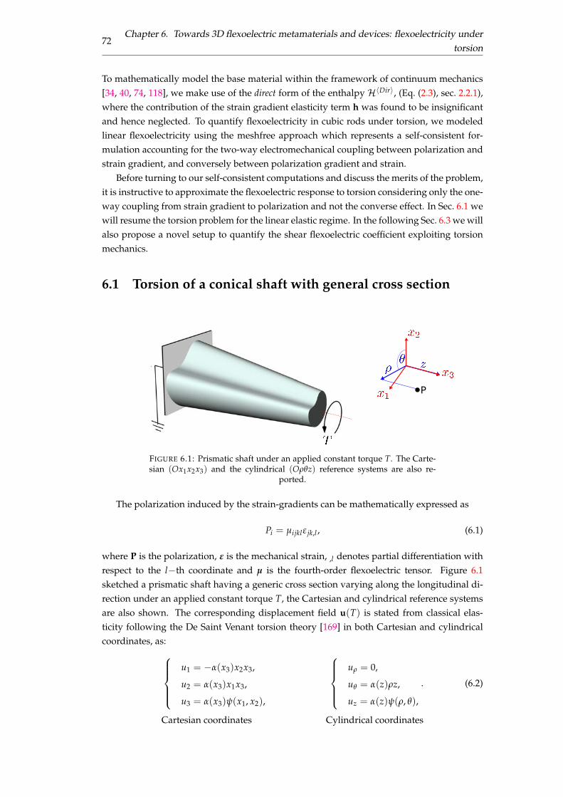
72Chapter 6. Towards 3D flexoelectric metamaterials and devices: flexoelectricity under
torsion
To mathematically model the base material within the framework of continuum mechanics[34, 40, 74, 118], we make use of the direct form of the enthalpy HhDiri, (Eq. (2.3), sec. 2.2.1),where the contribution of the strain gradient elasticity term h was found to be insignificantand hence neglected. To quantify flexoelectricity in cubic rods under torsion, we modeledlinear flexoelectricity using the meshfree approach which represents a self-consistent for-mulation accounting for the two-way electromechanical coupling between polarization andstrain gradient, and conversely between polarization gradient and strain.
Before turning to our self-consistent computations and discuss the merits of the problem,it is instructive to approximate the flexoelectric response to torsion considering only the one-way coupling from strain gradient to polarization and not the converse effect. In Sec. 6.1 wewill resume the torsion problem for the linear elastic regime. In the following Sec. 6.3 we willalso propose a novel setup to quantify the shear flexoelectric coefficient exploiting torsionmechanics.
6.1 Torsion of a conical shaft with general cross section
P
FIGURE 6.1: Prismatic shaft under an applied constant torque T. The Carte-sian (Ox1x2x3) and the cylindrical (Orqz) reference systems are also re-
ported.
The polarization induced by the strain-gradients can be mathematically expressed as
Pi = µijkl# jk,l , (6.1)
where P is the polarization, # is the mechanical strain, ,l denotes partial differentiation withrespect to the l�th coordinate and µ is the fourth-order flexoelectric tensor. Figure 6.1sketched a prismatic shaft having a generic cross section varying along the longitudinal di-rection under an applied constant torque T, the Cartesian and cylindrical reference systemsare also shown. The corresponding displacement field u(T) is stated from classical elas-ticity following the De Saint Venant torsion theory [169] in both Cartesian and cylindricalcoordinates, as:
8>>><
>>>:
u1 = �a(x3)x2x3,
u2 = a(x3)x1x3,
u3 = a(x3)y(x1, x2),
8>>><
>>>:
ur = 0,
uq = a(z)rz,
uz = a(z)y(r, q),
. (6.2)
Cartesian coordinates Cylindrical coordinates
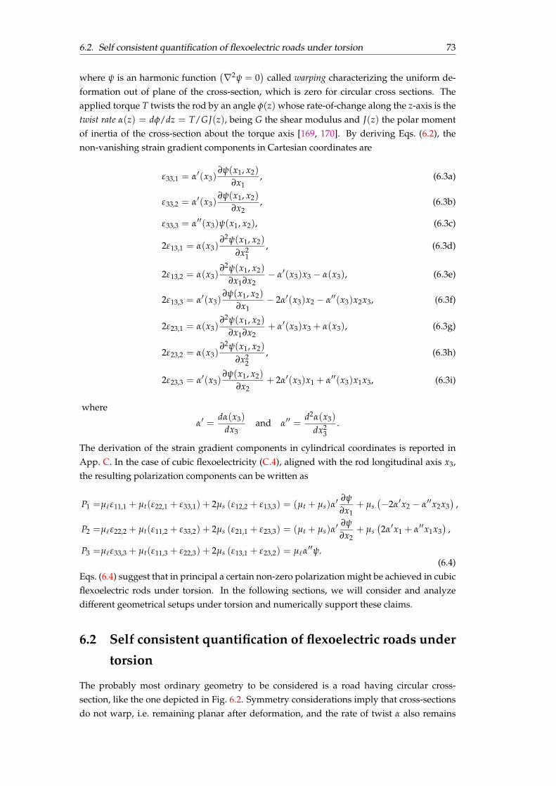
6.2. Self consistent quantification of flexoelectric roads under torsion 73
where y is an harmonic function�r2y = 0
�called warping characterizing the uniform de-
formation out of plane of the cross-section, which is zero for circular cross sections. Theapplied torque T twists the rod by an angle f(z) whose rate-of-change along the z-axis is thetwist rate a(z) = df/dz = T/GJ(z), being G the shear modulus and J(z) the polar momentof inertia of the cross-section about the torque axis [169, 170]. By deriving Eqs. (6.2), thenon-vanishing strain gradient components in Cartesian coordinates are
#33,1 = a0(x3)∂y(x1, x2)
∂x1, (6.3a)
#33,2 = a0(x3)∂y(x1, x2)
∂x2, (6.3b)
#33,3 = a00(x3)y(x1, x2), (6.3c)
2#13,1 = a(x3)∂2y(x1, x2)
∂x21
, (6.3d)
2#13,2 = a(x3)∂2y(x1, x2)
∂x1∂x2� a0(x3)x3 � a(x3), (6.3e)
2#13,3 = a0(x3)∂y(x1, x2)
∂x1� 2a0(x3)x2 � a00(x3)x2x3, (6.3f)
2#23,1 = a(x3)∂2y(x1, x2)
∂x1∂x2+ a0(x3)x3 + a(x3), (6.3g)
2#23,2 = a(x3)∂2y(x1, x2)
∂x22
, (6.3h)
2#23,3 = a0(x3)∂y(x1, x2)
∂x2+ 2a0(x3)x1 + a00(x3)x1x3, (6.3i)
where
a0 =da(x3)
dx3and a00 =
d2a(x3)
dx23
.
The derivation of the strain gradient components in cylindrical coordinates is reported inApp. C. In the case of cubic flexoelectricity (C.4), aligned with the rod longitudinal axis x3,the resulting polarization components can be written as
P1 =µ`#11,1 + µt(#22,1 + #33,1) + 2µs (#12,2 + #13,3) = (µt + µs)a0 ∂y
∂x1+ µs
��2a0x2 � a00x2x3
�,
P2 =µ`#22,2 + µt(#11,2 + #33,2) + 2µs (#21,1 + #23,3) = (µt + µs)a0 ∂y
∂x2+ µs
�2a0x1 + a00x1x3
�,
P3 =µ`#33,3 + µt(#11,3 + #22,3) + 2µs (#13,1 + #23,2) = µ`a00y.
(6.4)Eqs. (6.4) suggest that in principal a certain non-zero polarization might be achieved in cubicflexoelectric rods under torsion. In the following sections, we will consider and analyzedifferent geometrical setups under torsion and numerically support these claims.
6.2 Self consistent quantification of flexoelectric roads undertorsion
The probably most ordinary geometry to be considered is a road having circular cross-section, like the one depicted in Fig. 6.2. Symmetry considerations imply that cross-sectionsdo not warp, i.e. remaining planar after deformation, and the rate of twist a also remains
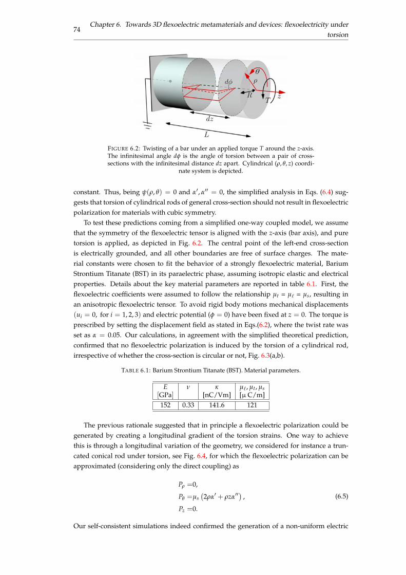
74Chapter 6. Towards 3D flexoelectric metamaterials and devices: flexoelectricity under
torsion
FIGURE 6.2: Twisting of a bar under an applied torque T around the z-axis.The infinitesimal angle df is the angle of torsion between a pair of cross-sections with the infinitesimal distance dz apart. Cylindrical (r, q, z) coordi-
nate system is depicted.
constant. Thus, being y(r, q) = 0 and a0, a00 = 0, the simplified analysis in Eqs. (6.4) sug-gests that torsion of cylindrical rods of general cross-section should not result in flexoelectricpolarization for materials with cubic symmetry.
To test these predictions coming from a simplified one-way coupled model, we assumethat the symmetry of the flexoelectric tensor is aligned with the z-axis (bar axis), and puretorsion is applied, as depicted in Fig. 6.2. The central point of the left-end cross-sectionis electrically grounded, and all other boundaries are free of surface charges. The mate-rial constants were chosen to fit the behavior of a strongly flexoelectric material, BariumStrontium Titanate (BST) in its paraelectric phase, assuming isotropic elastic and electricalproperties. Details about the key material parameters are reported in table 6.1. First, theflexoelectric coefficients were assumed to follow the relationship µt = µ` = µs, resulting inan anisotropic flexoelectric tensor. To avoid rigid body motions mechanical displacements(ui = 0, for i = 1, 2, 3) and electric potential (f = 0) have been fixed at z = 0. The torque isprescribed by setting the displacement field as stated in Eqs.(6.2), where the twist rate wasset as a = 0.05. Our calculations, in agreement with the simplified theoretical prediction,confirmed that no flexoelectric polarization is induced by the torsion of a cylindrical rod,irrespective of whether the cross-section is circular or not, Fig. 6.3(a,b).
TABLE 6.1: Barium Strontium Titanate (BST). Material parameters.
E n k µ`, µt, µs[GPa] [nC/Vm] [µ C/m]152 0.33 141.6 121
The previous rationale suggested that in principle a flexoelectric polarization could begenerated by creating a longitudinal gradient of the torsion strains. One way to achievethis is through a longitudinal variation of the geometry, we considered for instance a trun-cated conical rod under torsion, see Fig. 6.4, for which the flexoelectric polarization can beapproximated (considering only the direct coupling) as
Pr =0,
Pq =µs�2ra0 + rza00
�,
Pz =0.
(6.5)
Our self-consistent simulations indeed confirmed the generation of a non-uniform electric
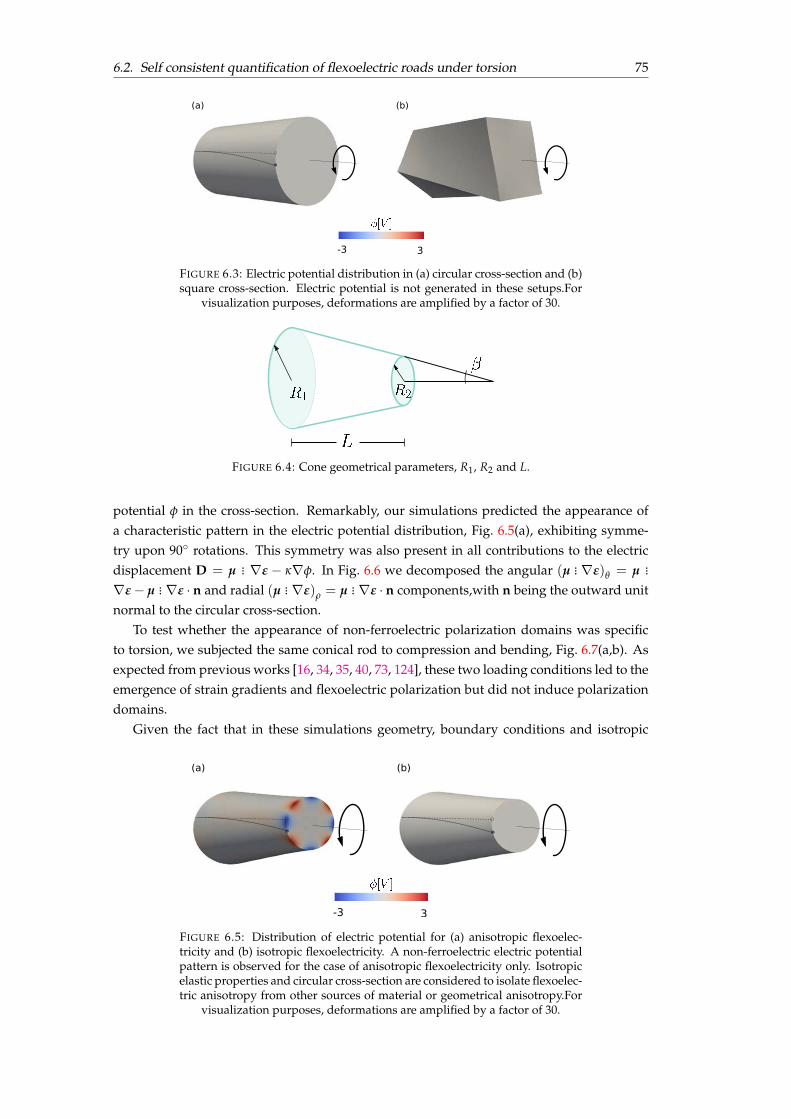
6.2. Self consistent quantification of flexoelectric roads under torsion 75
(a) (b)
-3 3
FIGURE 6.3: Electric potential distribution in (a) circular cross-section and (b)square cross-section. Electric potential is not generated in these setups.For
visualization purposes, deformations are amplified by a factor of 30.
FIGURE 6.4: Cone geometrical parameters, R1, R2 and L.
potential f in the cross-section. Remarkably, our simulations predicted the appearance ofa characteristic pattern in the electric potential distribution, Fig. 6.5(a), exhibiting symme-try upon 90� rotations. This symmetry was also present in all contributions to the electricdisplacement D = µ ... r# � krf. In Fig. 6.6 we decomposed the angular (µ ... r#)q = µ ...
r# � µ ... r# · n and radial (µ ... r#)r = µ ... r# · n components,with n being the outward unitnormal to the circular cross-section.
To test whether the appearance of non-ferroelectric polarization domains was specificto torsion, we subjected the same conical rod to compression and bending, Fig. 6.7(a,b). Asexpected from previous works [16, 34, 35, 40, 73, 124], these two loading conditions led to theemergence of strain gradients and flexoelectric polarization but did not induce polarizationdomains.
Given the fact that in these simulations geometry, boundary conditions and isotropic
(a) (b)
-3 3
FIGURE 6.5: Distribution of electric potential for (a) anisotropic flexoelec-tricity and (b) isotropic flexoelectricity. A non-ferroelectric electric potentialpattern is observed for the case of anisotropic flexoelectricity only. Isotropicelastic properties and circular cross-section are considered to isolate flexoelec-tric anisotropy from other sources of material or geometrical anisotropy.For
visualization purposes, deformations are amplified by a factor of 30.
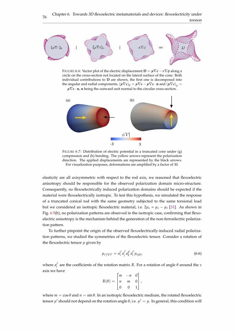
76Chapter 6. Towards 3D flexoelectric metamaterials and devices: flexoelectricity under
torsion
FIGURE 6.6: Vector plot of the electric displacement D = µr# � krf along acircle on the cross-section not located on the lateral surface of the cone. Bothindividual contributions to D are shown, the first one is decomposed intothe angular and radial components, (µr#)q = µr# � µr# · n and (µr#)r =
µr# · n, n being the outward unit normal to the circular cross-section.
(a) (b)
-3 3FIGURE 6.7: Distribution of electric potential in a truncated cone under (g)compression and (h) bending. The yellow arrows represent the polarizationdirection. The applied displacements are represented by the black arrows.
For visualization purposes, deformations are amplified by a factor of 30.
elasticity are all axisymmetric with respect to the rod axis, we reasoned that flexoelectricanisotropy should be responsible for the observed polarization domain micro-structure.Consequently, no flexoelectrically induced polarization domains should be expected if thematerial were flexoelectrically isotropic. To test this hypothesis, we simulated the responseof a truncated conical rod with the same geometry subjected to the same torsional loadbut we considered an isotropic flexoelectric material, i.e. 2µs = µ` � µt [31]. As shown inFig. 6.5(b), no polarization patterns are observed in the isotropic case, confirming that flexo-electric anisotropy is the mechanism behind the generation of the non-ferroelectric polariza-tion pattern.
To further pinpoint the origin of the observed flexoelectrically-induced radial polariza-tion patterns, we studied the symmetries of the flexoelectric tensor. Consider a rotation ofthe flexoelectric tensor µ given by
µi0 j0k0 l0 = ai0i aj0
j ak0k al0
l µijkl , (6.6)
where ai0i are the coefficients of the rotation matrix R. For a rotation of angle q around the z
axis we have
R(q) =
2
64m �n 0n m 00 0 1
3
75 ,
where m = cos q and n = sin q. In an isotropic flexoelectric medium, the rotated flexoelectrictensor µ0 should not depend on the rotation angle q, i.e. µ0 = µ. In general, this condition will
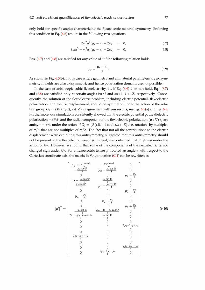
6.2. Self consistent quantification of flexoelectric roads under torsion 77
only hold for specific angles characterizing the flexoelectric material symmetry. Enforcingthis condition in Eq. (6.6) results in the following two equations:
2m2n2(µ` � µt � 2µs) = 0, (6.7)
(mn3 � m3n)(µ` � µt � 2µs) = 0. (6.8)
Eqs. (6.7) and (6.8) are satisfied for any value of q if the following relation holds
µs =µ` � µt
2. (6.9)
As shown in Fig. 6.5(b), in this case where geometry and all material parameters are axisym-metric, all fields are also axisymmetric and hence polarization domains are not possible.
In the case of anisotropic cubic flexoelectricity, i.e. if Eq. (6.9) does not hold, Eqs. (6.7)and (6.8) are satisfied only at certain angles kp/2 and kp/4, k 2 Z, respectively. Conse-quently, the solution of the flexoelectric problem, including electric potential, flexoelectricpolarization, and electric displacement, should be symmetric under the action of the rota-tion group G1 = {R(kp/2), k 2 Z} in agreement with our results, see Fig. 6.5(a) and Fig. 6.6.Furthermore, our simulations consistently showed that the electric potential f, the dielectricpolarization �krf, and the radial component of the flexoelectric polarization (µ ... r#)r areantisymmetric under the action of G2 = {R((2k + 1)p/4), k 2 Z}, i.e. rotations by multiplesof p/4 that are not multiples of p/2. The fact that not all the contributions to the electricdisplacement were exhibiting this antisymmetry, suggested that this antisymmetry shouldnot be present in the flexoelectric tensor µ. Indeed, we confirmed that µ0 6= �µ under theaction of G2. However, we found that some of the components of the flexoelectric tensorchanged sign under G2. For a flexoelectric tensor µ0 rotated an angle q with respect to theCartesian coordinate axis, the matrix in Voigt notation (C.4) can be rewritten as
[µ0]T =
2
6666666666666666666666666666666666666664
µ1 +µa cos 4q
4 � µa sin 4q4 0
� µa sin 4q4 µ2 � µa cos 4q
4 00 0 µ2 � µa
4µ2 � µa cos 4q
4µa sin 4q
4 0µa sin 4q
4 µ1 +µa cos 4q
4 00 0 µ2 � µa
4µ2 � µa
4 0 00 µ2 � µa
4 00 0 µ1 +
µa4
� µa sin 4q4
2µ1�2µ2�µa cos 4q4 0
2µ1�2µ2�µa cos 4q4
µa sin 4q4 0
0 0 00 0 2µ1�2µ2�µa
40 0 0
2µ1�2µ2�µa4 0 00 0 00 0 2µ1�2µ2�µa
40 2µ1�2µ2�µa
4 0
3
7777777777777777777777777777777777777775
, (6.10)
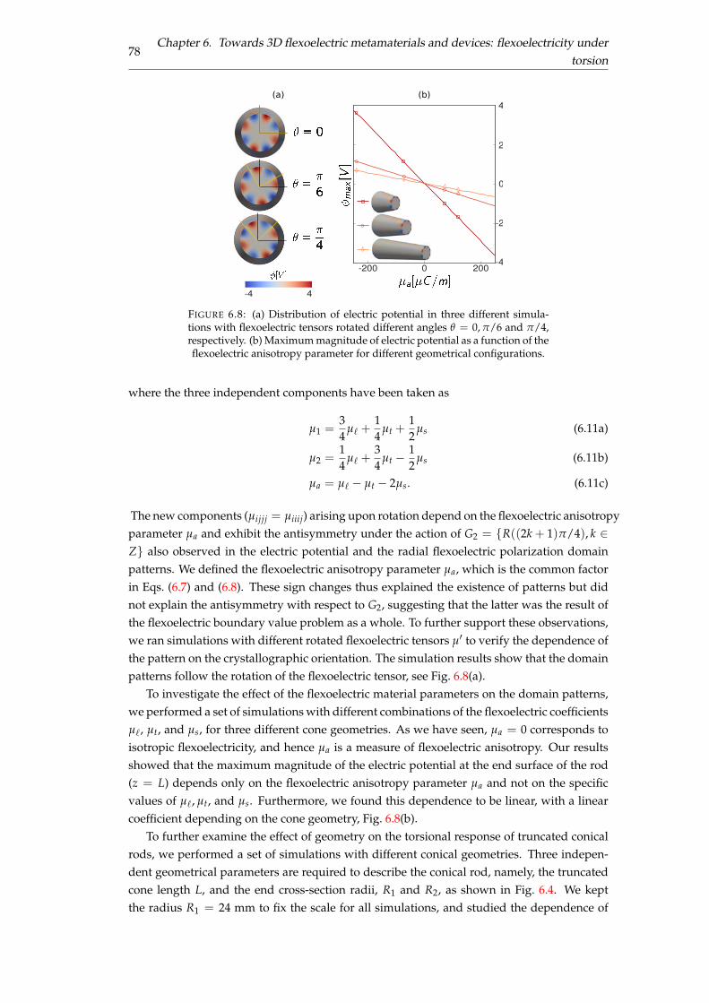
78Chapter 6. Towards 3D flexoelectric metamaterials and devices: flexoelectricity under
torsion
(a)
-4 4
(b)
2
4
0
-2
-4-200 0 200
FIGURE 6.8: (a) Distribution of electric potential in three different simula-tions with flexoelectric tensors rotated different angles q = 0, p/6 and p/4,respectively. (b) Maximum magnitude of electric potential as a function of theflexoelectric anisotropy parameter for different geometrical configurations.
where the three independent components have been taken as
µ1 =34
µ` +14
µt +12
µs (6.11a)
µ2 =14
µ` +34
µt �12
µs (6.11b)
µa = µ` � µt � 2µs. (6.11c)
The new components (µijjj = µiiij) arising upon rotation depend on the flexoelectric anisotropyparameter µa and exhibit the antisymmetry under the action of G2 = {R((2k + 1)p/4), k 2Z} also observed in the electric potential and the radial flexoelectric polarization domainpatterns. We defined the flexoelectric anisotropy parameter µa, which is the common factorin Eqs. (6.7) and (6.8). These sign changes thus explained the existence of patterns but didnot explain the antisymmetry with respect to G2, suggesting that the latter was the result ofthe flexoelectric boundary value problem as a whole. To further support these observations,we ran simulations with different rotated flexoelectric tensors µ0 to verify the dependence ofthe pattern on the crystallographic orientation. The simulation results show that the domainpatterns follow the rotation of the flexoelectric tensor, see Fig. 6.8(a).
To investigate the effect of the flexoelectric material parameters on the domain patterns,we performed a set of simulations with different combinations of the flexoelectric coefficientsµ`, µt, and µs, for three different cone geometries. As we have seen, µa = 0 corresponds toisotropic flexoelectricity, and hence µa is a measure of flexoelectric anisotropy. Our resultsshowed that the maximum magnitude of the electric potential at the end surface of the rod(z = L) depends only on the flexoelectric anisotropy parameter µa and not on the specificvalues of µ`, µt, and µs. Furthermore, we found this dependence to be linear, with a linearcoefficient depending on the cone geometry, Fig. 6.8(b).
To further examine the effect of geometry on the torsional response of truncated conicalrods, we performed a set of simulations with different conical geometries. Three indepen-dent geometrical parameters are required to describe the conical rod, namely, the truncatedcone length L, and the end cross-section radii, R1 and R2, as shown in Fig. 6.4. We keptthe radius R1 = 24 mm to fix the scale for all simulations, and studied the dependence of
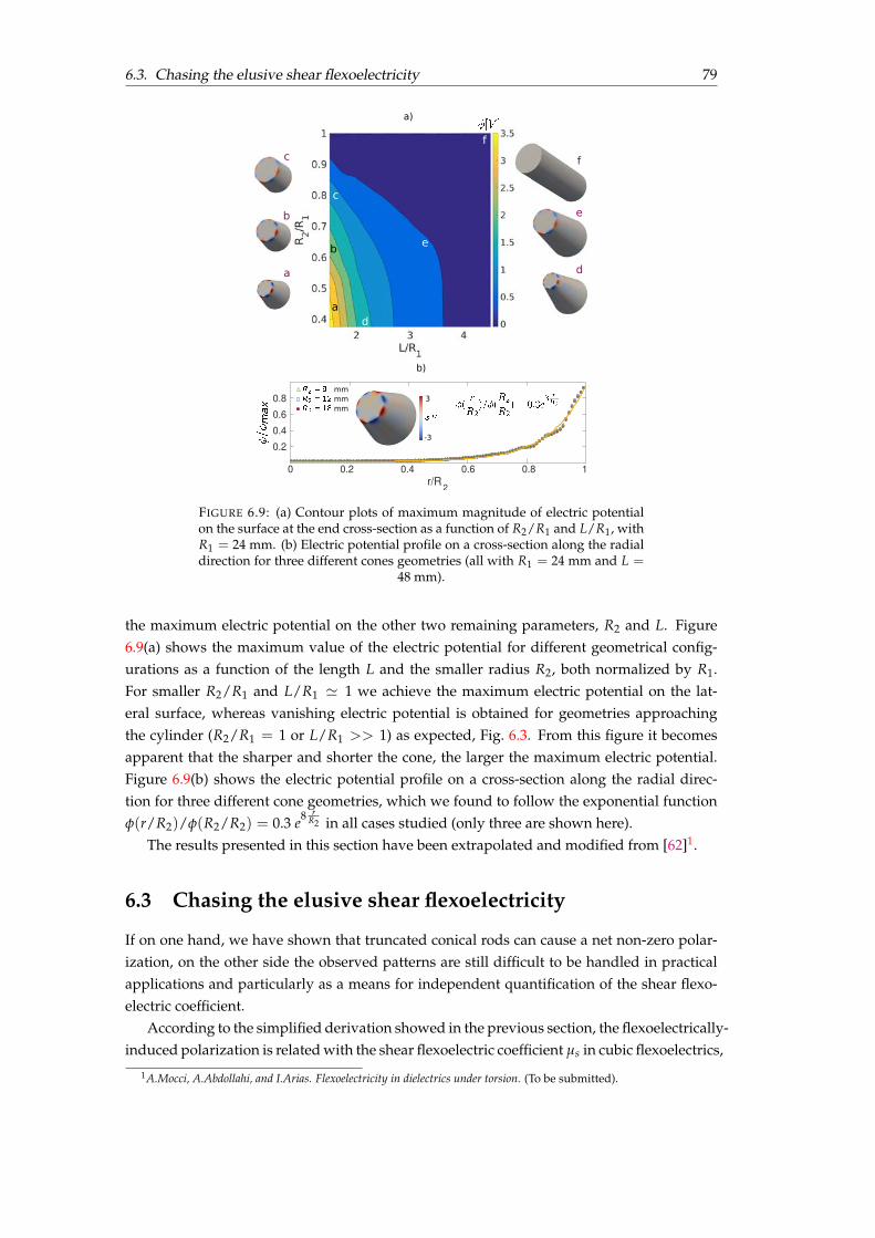
6.3. Chasing the elusive shear flexoelectricity 79
a)
a
b
c
d
e
f
a
b e
d
fc
b)
r/R 2
0 0.2 0.4 0.6 0.8 1
0.20.40.60.8
-3
3mmmmmm
FIGURE 6.9: (a) Contour plots of maximum magnitude of electric potentialon the surface at the end cross-section as a function of R2/R1 and L/R1, withR1 = 24 mm. (b) Electric potential profile on a cross-section along the radialdirection for three different cones geometries (all with R1 = 24 mm and L =
48 mm).
the maximum electric potential on the other two remaining parameters, R2 and L. Figure6.9(a) shows the maximum value of the electric potential for different geometrical config-urations as a function of the length L and the smaller radius R2, both normalized by R1.For smaller R2/R1 and L/R1 ' 1 we achieve the maximum electric potential on the lat-eral surface, whereas vanishing electric potential is obtained for geometries approachingthe cylinder (R2/R1 = 1 or L/R1 >> 1) as expected, Fig. 6.3. From this figure it becomesapparent that the sharper and shorter the cone, the larger the maximum electric potential.Figure 6.9(b) shows the electric potential profile on a cross-section along the radial direc-tion for three different cone geometries, which we found to follow the exponential functionf(r/R2)/f(R2/R2) = 0.3 e8 r
R2 in all cases studied (only three are shown here).The results presented in this section have been extrapolated and modified from [62]1.
6.3 Chasing the elusive shear flexoelectricity
If on one hand, we have shown that truncated conical rods can cause a net non-zero polar-ization, on the other side the observed patterns are still difficult to be handled in practicalapplications and particularly as a means for independent quantification of the shear flexo-electric coefficient.
According to the simplified derivation showed in the previous section, the flexoelectrically-induced polarization is related with the shear flexoelectric coefficient µs in cubic flexoelectrics,
1A.Mocci, A.Abdollahi, and I.Arias. Flexoelectricity in dielectrics under torsion. (To be submitted).
80Chapter 6. Towards 3D flexoelectric metamaterials and devices: flexoelectricity under
torsion
FIGURE 6.10: Truncated cone having radius R1, R2, respectively and length L.A ground electrode is placed on the clamped end of the shaft while a torque
T is applied on the free-end.
cf. Eq. (6.5). Torsion of conical rods can thus be used as a means for independent quantifi-cation of this elusive coefficient. In order to do this, we need to establish a simple relation-ship between the flexoelectrically-induced polarization Pq and the experimentally measuredelectric potential. However, in a flexoelectric material the polarization is related through theelectric displacement as
Di = �kf,i + µijkl# jk,l , (6.12)
where k is the dielectric constant. In a truncated conical rod, cf. Fig. 6.4, this relation cannotbe easily established and thus it is not suitable for quantification purposes. The angularpolarization Pq cannot be easily computed from surface measurements of f. Due to therotational symmetry of the cross-section, Dq is indeed free to take any value, complicatingthe quantification of Pq from the electric potential.
On the contrary, on a half truncated cone, free of surface charges, cf. Fig. 6.11, the angularelectric displacement Dq vanishes on the surface, and thus the angular polarization can beestimated as
Pq(r, z) = krqf ⇡ kf(r, 0, z)� f(r, p, z)
pr, (6.13)
where the electric potential f is obtained from the simulation results.On the other hand, considering Eqs. (6.3), the resulting one-way coupled polarization is
Pr = (µt + µs) a0∂y
∂r, (6.14a)
Pq = (µt + µs) a01r
∂y
∂q+ µs
�a00zr + 2a0r
�, (6.14b)
Pz = µ`a00y + µsar2y, (6.14c)
from which, an analytical approximation of the angular polarization Pq can be obtained as
Paq (r, z) =
4µsTGJs(z) R(z)
✓R1 � R2
L
◆r, (6.15)
where R1 and R2 are the radii of the fixed- and free-end cross-sections of the bar, respectively,L represents the length of the beam, see Fig. 6.10, Js(z) is the polar moment of inertia of thesemi-circular cross-section about the torque axis, and R(z) is the cross-section radius, whichwe assume to vary linearly, i.e. R(z) = (R2 � R1)z/L + R1. The analytical estimation of theangular polarization in Eq. (6.15) bring along with two main simplifying assumptions. First,
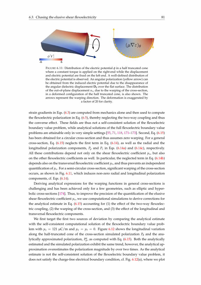
6.3. Chasing the elusive shear flexoelectricity 81
-6 6
FIGURE 6.11: Distribution of the electric potential f in a half truncated conewhere a constant torque is applied on the right-end while the displacementand electric potential are fixed on the left end. A well-defined distribution ofthe electric potential is observed. An angular polarization (yellow arrow) canbe obtained from the induced electric potential due to the disappearance ofthe angular dielectric displacement Dq over the flat surface. The distributionof the out-of-plane displacement uz, due to the warping of the cross-section,in a deformed configuration of the half truncated cone, is also shown. Thearrows represent the warping direction. The deformation is exaggerated by
a factor of 20 for clarity.
strain gradients in Eqs. (6.3) are computed from mechanics alone and then used to computethe flexoelectric polarization in Eq. (6.5), thereby neglecting the two-way coupling and thusthe converse effect. These fields are thus not a self-consistent solution of the flexoelectricboundary value problem, while analytical solutions of the full flexoelectric boundary valueproblems are attainable only in very simple settings [55, 71, 118, 171–173]. Second, Eq. (6.15)has been obtained for a circular cross-section and thus assumes zero warping. For a generalcross-section, Eq. (6.15) neglects the first term in Eq. (6.14), as well as the radial and thelongitudinal polarization components, Pr and Pz in Eqs. (6.14a) and (6.14c), respectively.All these contributions depend not only on the shear flexoelectric coefficient µs, but alsoon the other flexoelectric coefficients as well. In particular, the neglected term in Eq. (6.14b)depends also on the transversal flexoelectric coefficient µt, and thus prevents an independentquantification of µs. For a semi-circular cross-section, significant warping of the cross-sectionoccurs, as shown in Fig. 6.11, which induces non-zero radial and longitudinal polarizationcomponents, cf. Eqs. (6.14).
Deriving analytical expressions for the warping functions in general cross-sections ischallenging and has been achieved only for a few geometries, such as elliptic and hyper-bolic cross-sections [174]. Thus, to improve the precision of the quantification of the elusiveshear flexoelectric coefficient µs, we use computational simulations to derive corrections forthe analytical estimate in Eq. (6.15) accounting for (1) the effect of the two-way flexoelec-tric coupling, (2) the warping of the cross-section, and (3) the effect of the longitudinal andtransversal flexoelectric components.
We first target the first two sources of deviation by comparing the analytical estimatewith the self-consistent computational solution of the flexoelectric boundary value prob-lem with µs = 121 µC/m and µ` = µt = 0. Figure 6.12 shows the longitudinal variationalong the half-truncated cone of the cross-section simulated polarization Pq and the ana-lytically approximated polarization, Pa
q , as computed with Eq. (6.15). Both the analyticallyestimated and the simulated polarization exhibit the same trend, however, the analytical ap-proximation overestimates the polarization magnitude by over two times. As the analyticalestimate is not the self-consistent solution of the flexoelectric boundary value problem, itdoes not satisfy the charge-free electrical boundary condition, cf. Fig. 6.12(a), where we plot
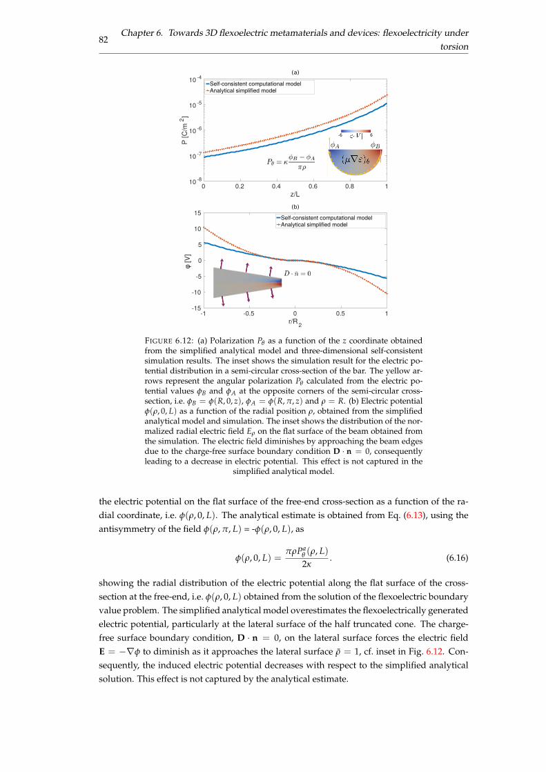
82Chapter 6. Towards 3D flexoelectric metamaterials and devices: flexoelectricity under
torsion
-1 -0.5 0 0.5 1r/R2
-15
-10
-5
0
5
10
15
�[V
]
Self-consistent computational modelAnalytical simplified model
(b)
0 0.2 0.4 0.6 0.8 1z/L
10 -8
10 -7
10 -6
10 -5
10 -4
P [C
/m2 ]
Self-consistent computational modelAnalytical simplified model
-6 6
(a)
FIGURE 6.12: (a) Polarization Pq as a function of the z coordinate obtainedfrom the simplified analytical model and three-dimensional self-consistentsimulation results. The inset shows the simulation result for the electric po-tential distribution in a semi-circular cross-section of the bar. The yellow ar-rows represent the angular polarization Pq calculated from the electric po-tential values fB and fA at the opposite corners of the semi-circular cross-section, i.e. fB = f(R, 0, z), fA = f(R, p, z) and r = R. (b) Electric potentialf(r, 0, L) as a function of the radial position r, obtained from the simplifiedanalytical model and simulation. The inset shows the distribution of the nor-malized radial electric field Er on the flat surface of the beam obtained fromthe simulation. The electric field diminishes by approaching the beam edgesdue to the charge-free surface boundary condition D · n = 0, consequentlyleading to a decrease in electric potential. This effect is not captured in the
simplified analytical model.
the electric potential on the flat surface of the free-end cross-section as a function of the ra-dial coordinate, i.e. f(r, 0, L). The analytical estimate is obtained from Eq. (6.13), using theantisymmetry of the field f(r, p, L) = -f(r, 0, L), as
f(r, 0, L) =prPa
q (r, L)2k
. (6.16)
showing the radial distribution of the electric potential along the flat surface of the cross-section at the free-end, i.e. f(r, 0, L) obtained from the solution of the flexoelectric boundaryvalue problem. The simplified analytical model overestimates the flexoelectrically generatedelectric potential, particularly at the lateral surface of the half truncated cone. The charge-free surface boundary condition, D · n = 0, on the lateral surface forces the electric fieldE = �rf to diminish as it approaches the lateral surface r = 1, cf. inset in Fig. 6.12. Con-sequently, the induced electric potential decreases with respect to the simplified analyticalsolution. This effect is not captured by the analytical estimate.
6.3. Chasing the elusive shear flexoelectricity 83
We define the deviation of the estimate with respect to the self-consistent solution as
D(r, z; R1, R2, L, E, n, k, µ`, µt, µs) =Pa
q (r, z; R1, R2, L, E, n, µs)
Pq(r, z; R1, R2, L, E, n, k, µ`, µt, µs), (6.17)
where Pq and Paq are given in Eqs. (6.13) and (6.15), respectively. To systematically study
this deviation, we perform a number of simulations considering different geometries andmaterial parameters. We have observed a small variation in D (not shown) by changing theconfiguration and elastic properties, since the corresponding parameters R1, R2, L, Js andG have already encoded these changes in the analytical model in Eq. (6.15). However, aconsiderable variation in D occurs by considering non-zero values for the longitudinal µ`
and transversal µt coefficients of flexoelectricity. The main reason is due to additional effectsof warping since the out-of-plane displacement uz induces other non-zero strain gradientcomponents as reported in Eqs. (6.3), which in turn activate the longitudinal and transversalcomponents of flexoelectricity, contaminating the pure shear flexoelectric response. Sincethe strongest response is induced over the free-end semi-circular surface, we quantify thedeviation Dv = D(R2, L) by performing a number of simulations using different values ofµ` and µt. Figure 6.13(a) presents the results which can be summarized by the following fit:
Dv(µ`, µt) = f00 + f10µ` + f01µt + f20µ2` + f11µ`µt (6.18)
+ f02µ2t + f30µ3
` + f21µ2`µt + f12µ`µ
2t + f03µ3
t (6.19)
+ f31µ3`µt + f22µ2
`µ2t + f13µ`µ
3t + f04µ4
t , (6.20)
where the f coefficients are presented in Table 6.2. A noticeable deviation is observed inFig. 6.13(b) by considering a non-zero value for either the flexoelectric coefficient µ` or µt.Equation (6.20) provides a practical way to quantify this deviation and correct the simplifiedanalytical estimation in Eq. (6.15).
TABLE 6.2: f coefficients
f00 f10 f01 f20 f11 f02 f302.09 21.97 -19 160.6 -271.8 90.11 224.1f21 f12 f03 f31 f22 f13 f04
-119.5 -493.1 230.3 7878 �1.641e4 7993 2222
Finally, after providing an analytical expression for the deviation, we suggest a methodto quantify the shear flexoelectric coefficient µs. This is done by expanding and rearrangingEq. (6.17) using Eqs. (6.13) and (6.15) as
µs =kDvLJsGDf
4pTR2(R1 � R2), (6.21)
where Df = f(R2, 0, L)� f(R2, p, L). This equation could be employed for two purposes:
• To validate computational models of flexoelectricity. In this case, by considering thesame parameters of the simulation model and the voltage difference Df obtained fromthe simulation results, Eq. (6.21) should give the same value of µs used in the simula-tion, in order to validate the model.
• To quantify the shear flexoelectric coefficient µs from experimental measurements. Byusing the configuration and material parameters of the sample, the applied torque
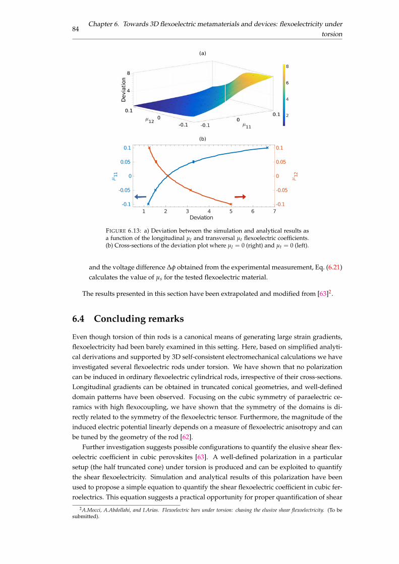
84Chapter 6. Towards 3D flexoelectric metamaterials and devices: flexoelectricity under
torsion
1 2 3 4 5 6 7Deviation
-0.1
-0.05
0
0.05
0.1
11
-0.1
-0.05
0
0.05
0.1
12
(b)
(a)
FIGURE 6.13: a) Deviation between the simulation and analytical results asa function of the longitudinal µl and transversal µt flexoelectric coefficients.(b) Cross-sections of the deviation plot where µl = 0 (right) and µt = 0 (left).
and the voltage difference Df obtained from the experimental measurement, Eq. (6.21)calculates the value of µs for the tested flexoelectric material.
The results presented in this section have been extrapolated and modified from [63]2.
6.4 Concluding remarks
Even though torsion of thin rods is a canonical means of generating large strain gradients,flexoelectricity had been barely examined in this setting. Here, based on simplified analyti-cal derivations and supported by 3D self-consistent electromechanical calculations we haveinvestigated several flexoelectric rods under torsion. We have shown that no polarizationcan be induced in ordinary flexoelectric cylindrical rods, irrespective of their cross-sections.Longitudinal gradients can be obtained in truncated conical geometries, and well-defineddomain patterns have been observed. Focusing on the cubic symmetry of paraelectric ce-ramics with high flexocoupling, we have shown that the symmetry of the domains is di-rectly related to the symmetry of the flexoelectric tensor. Furthermore, the magnitude of theinduced electric potential linearly depends on a measure of flexoelectric anisotropy and canbe tuned by the geometry of the rod [62].
Further investigation suggests possible configurations to quantify the elusive shear flex-oelectric coefficient in cubic perovskites [63]. A well-defined polarization in a particularsetup (the half truncated cone) under torsion is produced and can be exploited to quantifythe shear flexoelectricity. Simulation and analytical results of this polarization have beenused to propose a simple equation to quantify the shear flexoelectric coefficient in cubic fer-roelectrics. This equation suggests a practical opportunity for proper quantification of shear
2A.Mocci, A.Abdollahi, and I.Arias. Flexoelectric bars under torsion: chasing the elusive shear flexoelectricity. (To besubmitted).

6.4. Concluding remarks 85
flexoelectricity as well as a validation benchmark for computational models of flexoelectric-ity.

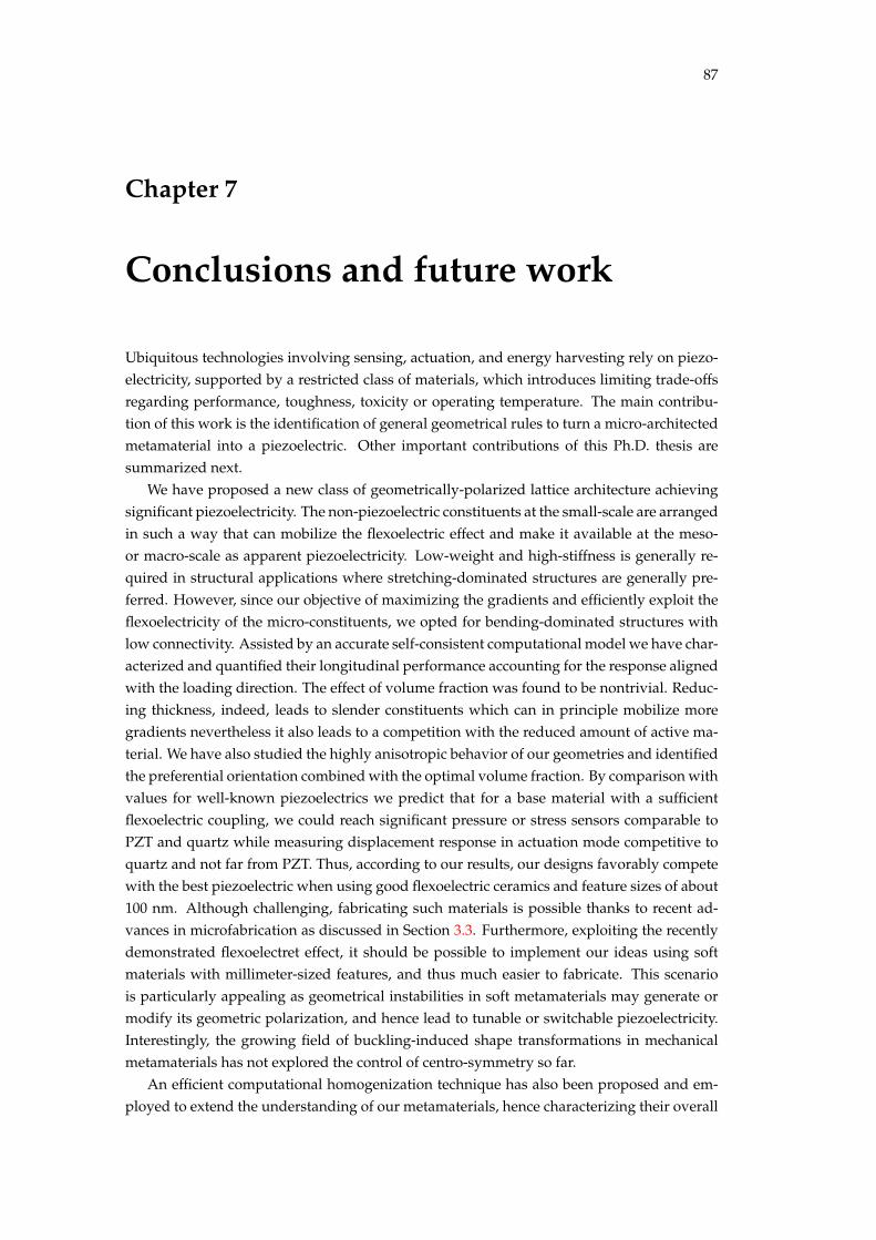
87
Chapter 7
Conclusions and future work
Ubiquitous technologies involving sensing, actuation, and energy harvesting rely on piezo-electricity, supported by a restricted class of materials, which introduces limiting trade-offsregarding performance, toughness, toxicity or operating temperature. The main contribu-tion of this work is the identification of general geometrical rules to turn a micro-architectedmetamaterial into a piezoelectric. Other important contributions of this Ph.D. thesis aresummarized next.
We have proposed a new class of geometrically-polarized lattice architecture achievingsignificant piezoelectricity. The non-piezoelectric constituents at the small-scale are arrangedin such a way that can mobilize the flexoelectric effect and make it available at the meso-or macro-scale as apparent piezoelectricity. Low-weight and high-stiffness is generally re-quired in structural applications where stretching-dominated structures are generally pre-ferred. However, since our objective of maximizing the gradients and efficiently exploit theflexoelectricity of the micro-constituents, we opted for bending-dominated structures withlow connectivity. Assisted by an accurate self-consistent computational model we have char-acterized and quantified their longitudinal performance accounting for the response alignedwith the loading direction. The effect of volume fraction was found to be nontrivial. Reduc-ing thickness, indeed, leads to slender constituents which can in principle mobilize moregradients nevertheless it also leads to a competition with the reduced amount of active ma-terial. We have also studied the highly anisotropic behavior of our geometries and identifiedthe preferential orientation combined with the optimal volume fraction. By comparison withvalues for well-known piezoelectrics we predict that for a base material with a sufficientflexoelectric coupling, we could reach significant pressure or stress sensors comparable toPZT and quartz while measuring displacement response in actuation mode competitive toquartz and not far from PZT. Thus, according to our results, our designs favorably competewith the best piezoelectric when using good flexoelectric ceramics and feature sizes of about100 nm. Although challenging, fabricating such materials is possible thanks to recent ad-vances in microfabrication as discussed in Section 3.3. Furthermore, exploiting the recentlydemonstrated flexoelectret effect, it should be possible to implement our ideas using softmaterials with millimeter-sized features, and thus much easier to fabricate. This scenariois particularly appealing as geometrical instabilities in soft metamaterials may generate ormodify its geometric polarization, and hence lead to tunable or switchable piezoelectricity.Interestingly, the growing field of buckling-induced shape transformations in mechanicalmetamaterials has not explored the control of centro-symmetry so far.
An efficient computational homogenization technique has also been proposed and em-ployed to extend the understanding of our metamaterials, hence characterizing their overall
88 Chapter 7. Conclusions and future work
behavior. Due to this comprehensive analysis, we were able to identify the preferred oper-ation mode for each design. Indeed, we spot that the longitudinal piezoelectric coefficientwas not necessarily the larger for each design, but instead, the lattices exhibiting lower sym-metries might perform better in shear or transverse mode.
We presented a systematic shape and material optimization study based on gradientand genetic algorithms. We concluded that more compliant designs able to accommodatethe deformations are thus extremely suitable for stress sensors for which we predict perfor-mances comparable to the best piezoelectrics. We find a similar situation for actuators whendisplacements are measured. On the contrary, the competition between slenderness andamount of materials is evidently in favor of the latter when displacements are imposed orstress is measured. For these setups, stiffer structures with small unit cells and well-orientedconstituents are preferred. However, we end by highlighting that low-area fraction latticesare ultimately not appropriate for measuring the stress mobilized by an applied electric field.
Besides imprinting polarity geometrically in a lattice metamaterial, the overall symmetryof the system can be broken through multimaterial arrangements and boundary conditions.This concept was explored in detail and designs for flexoelectric devices combining twomaterials were proposed, analyzed and quantified.
In view of extending our work to 3D we focused on establishing new building blocks forthree-dimensional metamaterials involving more complex ways of mobilizing gradients. Wepresented a comprehensive study of flexoelectric rods under torsion in cubic ferroelectrics.As predicted by a simplified analytical calculation, the 3D self-consistent computational ap-proach confirmed that no flexoelectric polarization can be induced in trivial geometricalsetups such as cylindrical rods subjected to a constant torque. The longitudinal gradientinduced by varying cross-sections along the rods axis leads to well-defined polarization do-mains in truncated conical rods under torsion. We have demonstrated that the symmetryof the polarization domains is directly related to the symmetry of the flexoelectric tensor,whereas a measure of its anisotropy determines its magnitude, which can be tuned by thegeometrical parameters of the rod. In further investigations, we also suggested other possi-ble configurations, such as the half truncated cone under torsion where a well-defined po-larization was induced. This configuration was proposed as a means to quantify the shearflexoelectric coefficient. In addition, it represents and has been used [59] as a validationbenchmark for computational models of flexoelectricity.
7.1 Future work
In this Ph.D. thesis, we have broadly investigated the behavior of the proposed 2D low-areafraction bending-dominated lattices. During the investigation process, we gained mean-ingful insights, nonetheless the final objective of this work would naturally be to extendour knowledge to 3D, where we expect that our designs may further enhance the effectivepiezoelectricity.
In two-dimension the topological design of our rational metamaterials was mainly guidedby intuition, however, in 3D the design space for optimal concepts able to attain substantialeffective piezoelectricity might be challenging to achieve. Topological rearrangements and
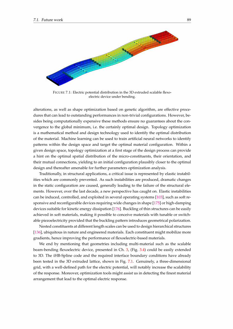
7.1. Future work 89
FIGURE 7.1: Electric potential distribution in the 3D extruded scalable flexo-electric device under bending.
alterations, as well as shape optimization based on genetic algorithm, are effective proce-dures that can lead to outstanding performances in non-trivial configurations. However, be-sides being computationally expensive these methods ensure no guarantees about the con-vergence to the global minimum, i.e. the certainly optimal design. Topology optimizationis a mathematical method and design technology used to identify the optimal distributionof the material. Machine learning can be used to train artificial neural networks to identifypatterns within the design space and target the optimal material configuration. Within agiven design space, topology optimization at a first stage of the design process can providea hint on the optimal spatial distribution of the micro-constituents, their orientation, andtheir mutual connections, yielding to an initial configuration plausibly closer to the optimaldesign and thereafter amenable for further parameters optimization analysis.
Traditionally, in structural applications, a critical issue is represented by elastic instabil-ities which are commonly prevented. As such instabilities are produced, dramatic changesin the static configuration are caused, generally leading to the failure of the structural ele-ments. However, over the last decade, a new perspective has caught on. Elastic instabilitiescan be induced, controlled, and exploited in several operating systems [103], such as soft re-sponsive and reconfigurable devices requiring wide changes in shape [175] or high-dampingdevices suitable for kinetic energy dissipation [176]. Buckling of thin structures can be easilyachieved in soft materials, making it possible to conceive materials with tunable or switch-able piezoelectricity provided that the buckling pattern introduces geometrical polarization.
Nested constituents at different length scales can be used to design hierarchical structures[136], ubiquitous in nature and engineered materials. Each constituent might mobilize moregradients, hence improving the performance of flexoelectric-based materials.
We end by mentioning that geometries including multi-material such as the scalablebeam-bending flexoelectric device, presented in Ch. 3, (Fig. 3.4) could be easily extendedto 3D. The iHB-Spline code and the required interface boundary conditions have alreadybeen tested in the 3D extruded lattice, shown in Fig. 7.1. Genuinely, a three-dimensionalgrid, with a well-defined path for the electric potential, will notably increase the scalabilityof the response. Moreover, optimization tools might assist us in detecting the finest materialarrangement that lead to the optimal electric response.

91
Appendix A
Immersed boundary B-Splineframework
A.1 Material tensors
The material properties involved in the electromechanical bulk enthalpy defined in Eq. (2.2.1)and (2.2.2) are characterized by specifying the material tensors. Only non-zero componentsare specified.
Elasticity tensor C
The fourth-order tensor C characterizing isotropic elasticity is given by
Ciiii = Cl , i = 1, 2,
Ciijj = Ct, i, j = 1, 2 with i 6= j, (A.1)
Cijij = Cijji = Cs, i, j = 1, 2 with i 6= j,
with Cl , Ct and Cs defined in 2D plain strain condition in terms of Young’s modulus Y andPoisson’s ratio n as
Cl =Y(1 � n)
(1 + n)(1 � 2n), Ct =
Yn
(1 + n)(1 � 2n), Cs =
Y2(1 + n)
. (A.2)
Strain gradient elasticity tensor h
A simplified form of isotropic strain-gradient elasticity is used, allowing us to write thesixth-rank strain-gradient tensor h in terms of these elastic parameters and a length-scale`mech [177, 178] as
hiikiik = `2mechCl , i, k = 1, 2,
hiikjjk = `2mechCt, i, j, k = 1, 2 with i 6= j, (A.3)
hijkijk = hijkjik = `2mechCs, i, j, k = 1, 2 with i 6= j.
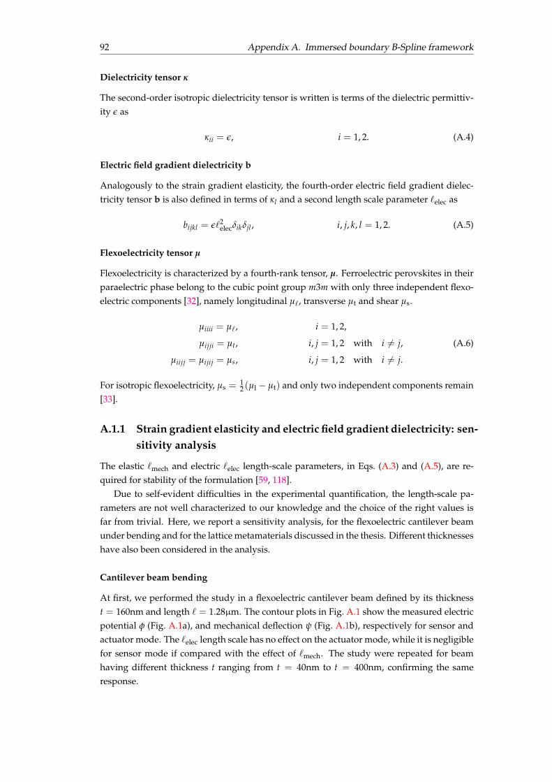
92 Appendix A. Immersed boundary B-Spline framework
Dielectricity tensor k
The second-order isotropic dielectricity tensor is written is terms of the dielectric permittiv-ity e as
kii = e, i = 1, 2. (A.4)
Electric field gradient dielectricity b
Analogously to the strain gradient elasticity, the fourth-order electric field gradient dielec-tricity tensor b is also defined in terms of kl and a second length scale parameter `elec as
bijkl = e`2elecdikdjl , i, j, k, l = 1, 2. (A.5)
Flexoelectricity tensor µ
Flexoelectricity is characterized by a fourth-rank tensor, µ. Ferroelectric perovskites in theirparaelectric phase belong to the cubic point group m3m with only three independent flexo-electric components [32], namely longitudinal µ`, transverse µt and shear µs.
µiiii = µ`, i = 1, 2,
µijji = µt, i, j = 1, 2 with i 6= j, (A.6)
µiijj = µijij = µs, i, j = 1, 2 with i 6= j.
For isotropic flexoelectricity, µs = 12 (µl � µt) and only two independent components remain
[33].
A.1.1 Strain gradient elasticity and electric field gradient dielectricity: sen-sitivity analysis
The elastic `mech and electric `elec length-scale parameters, in Eqs. (A.3) and (A.5), are re-quired for stability of the formulation [59, 118].
Due to self-evident difficulties in the experimental quantification, the length-scale pa-rameters are not well characterized to our knowledge and the choice of the right values isfar from trivial. Here, we report a sensitivity analysis, for the flexoelectric cantilever beamunder bending and for the lattice metamaterials discussed in the thesis. Different thicknesseshave also been considered in the analysis.
Cantilever beam bending
At first, we performed the study in a flexoelectric cantilever beam defined by its thicknesst = 160nm and length ` = 1.28µm. The contour plots in Fig. A.1 show the measured electricpotential f (Fig. A.1a), and mechanical deflection y (Fig. A.1b), respectively for sensor andactuator mode. The `elec length scale has no effect on the actuator mode, while it is negligiblefor sensor mode if compared with the effect of `mech. The study were repeated for beamhaving different thickness t ranging from t = 40nm to t = 400nm, confirming the sameresponse.
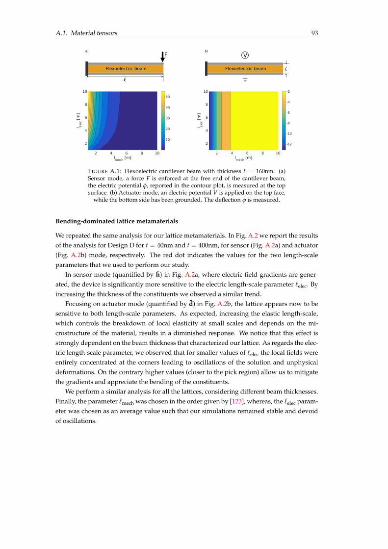
A.1. Material tensors 93
a) b)
Flexoelectric beam
F V
Flexoelectric beam
FIGURE A.1: Flexoelectric cantilever beam with thickness t = 160nm. (a)Sensor mode, a force F is enforced at the free end of the cantilever beam,the electric potential f, reported in the contour plot, is measured at the topsurface. (b) Actuator mode, an electric potential V is applied on the top face,
while the bottom side has been grounded. The deflection j is measured.
Bending-dominated lattice metamaterials
We repeated the same analysis for our lattice metamaterials. In Fig. A.2 we report the resultsof the analysis for Design D for t = 40nm and t = 400nm, for sensor (Fig. A.2a) and actuator(Fig. A.2b) mode, respectively. The red dot indicates the values for the two length-scaleparameters that we used to perform our study.
In sensor mode (quantified by h) in Fig. A.2a, where electric field gradients are gener-ated, the device is significantly more sensitive to the electric length-scale parameter `elec. Byincreasing the thickness of the constituents we observed a similar trend.
Focusing on actuator mode (quantified by d) in Fig. A.2b, the lattice appears now to besensitive to both length-scale parameters. As expected, increasing the elastic length-scale,which controls the breakdown of local elasticity at small scales and depends on the mi-crostructure of the material, results in a diminished response. We notice that this effect isstrongly dependent on the beam thickness that characterized our lattice. As regards the elec-tric length-scale parameter, we observed that for smaller values of `elec the local fields wereentirely concentrated at the corners leading to oscillations of the solution and unphysicaldeformations. On the contrary higher values (closer to the pick region) allow us to mitigatethe gradients and appreciate the bending of the constituents.
We perform a similar analysis for all the lattices, considering different beam thicknesses.Finally, the parameter `mech was chosen in the order given by [123], whereas, the `elec param-eter was chosen as an average value such that our simulations remained stable and devoidof oscillations.
94 Appendix A. Immersed boundary B-Spline framework
thickness (nm)
40
400
a) b)
FIGURE A.2: Sensitivity analysis for Design D, with t = 40nm and t =400nm.
95
Appendix B
Piezoelectric coefficients andboundary conditions derivation forthe homogenized RVE
B.1 Piezoelectricity
In Eq. (3.1) we introduced four effective piezoelectric coupling coefficients to quantify theresponse of our metamaterials, each of them pertinent to a distinct sensing or actuation sce-nario and derived from a different form of the energy based upon different choice or set ofindependent variables, namely, stress, strain, electric field and electric displacement. Thetransition from one set to another is accomplished by the so called Legendre transformation.
The electric enthalpy H, to which we mostly refer in this manuscript, leads to the directderivation of e. Here, for completeness we will report the derivation of the four piezoelec-tric coefficients. Note that the aforementioned derivation follows classical piezoelectricity[5] and therefore in this section we will not refer to effective properties. The energy formsdescribe a piezoelectric (non-flexoelectric) uniform material.
B.1.1 Energy forms
Internal energy U (#, D), h-form
The incremental change in the internal energy U for a dielectric elastic body subjected tosmall changes in the strains and electric displacements is defined as:
dU (#ij, Di) = sij d#ij + Ei dDi. (B.1)
In this form of the energy the independent set of the variables are strain and electric dis-placement (#kl , Dk) . We can thus write the total derivative form of the strain energy densityU as
dU (#ij, Di) =∂U∂#ij
�����D
d#ij +∂U∂Di
�����#
dDi. (B.2)
Upon comparing (B.1) and (B.2),
∂U∂#ij
�����D
= sij,∂U∂Di
�����#
= Ei. (B.3)
96Appendix B. Piezoelectric coefficients and boundary conditions derivation for the
homogenized RVE
Since (#, D) are independent variables, it implies that stresses and electric fields can be re-lated to strains and electric displacements as:
dsij(#kl , Dk) =∂sij
∂#kl
�����D
d#kl +∂sij
∂Dk
�����#
dDk, (B.4)
dEi(#kl , Dk) =∂Ei∂#kl
�����D
d#kl +∂Ei∂Dk
�����#
dDk. (B.5)
This leads to the standard definition of the third-order piezoelectric tensor h for both thedirect and converse effect
hkij = �∂sij
∂Dk
�����#
= � ∂
∂Dk
�����#
∂U∂#ij
�����D
= � ∂
∂#ij
✓∂U∂Dk
◆ �����#
! �����D
= �∂Ek∂#ij
�����D
. (B.6)
Gibbs energy F (s, E), d-form
To convert the independent set of variables from strain and electric displacement (#ij, Di)to stress and electric field (sij, Ei), we use Legendre Transformation. Hence we define a newfunction F (Gibbs function) as
F(sij, Ei) = U � sij#ij � EiDi. (B.7)
Upon differentiating the above equation and substituting (B.1), we obtain:
dF(sij, Ei) = �#ij dsij � Di dEi. (B.8)
Hence, we again notice that F now solely depends on (sij, Ei), therefore its total derivativeappears as
dF(sij, Ei) =∂F∂sij
�����E
dsij +∂F∂Ei
�����s
dEi. (B.9)
Thus, upon comparing,
∂F∂sij
�����E
= �#ij,∂F∂Ei
�����s
= �Di. (B.10)
As (s, E) are independent variables, it implies that strains and electric displacements can berelated to stresses and electric fields as
d#ij(skl , Ek) =∂#ij
∂skl
�����E
dskl +∂#ij
∂Ek
�����s
dEk, (B.11)
dDi(skl , Ek) =∂Di∂skl
�����E
dskl +∂Di∂Ek
�����s
dEk. (B.12)
B.1. Piezoelectricity 97
It follows the definition of the third-order piezoelectric tensor d for both the direct and con-verse effect
dkij =∂#ij
∂Ek
�����s
= �
∂
∂sij
✓∂F∂Ek
◆ �����s
! �����E
=∂Dk∂sij
�����E
. (B.13)
Electric enthalpy H (#, E), e-form
To convert the independent set of variables from strain and electric displacement (#ij, Di)to strain and electric field (#ij, Ei), we use Legendre Transformation. Hence we define a newfunction H (electric enthalpy) as
H(#ij, Ei) = U � DiEi. (B.14)
Upon differentiating the above equation and substituting (B.1), we obtain:
dH(#ij, Ei) = sijd#ij � DidEi. (B.15)
The electric enthalpy H now solely depends on (#ij, Ei), therefore its total derivative appearsas
dH(#ij, Ei) =∂H∂#ij
�����E
d#ij +∂H∂Ei
�����#
dEi. (B.16)
Thus, upon comparing,
∂H∂#ij
�����E
= sij,∂H∂Ei
�����#
= �Di. (B.17)
Being (#, E) independent state variables, it implies that stresses and dielectric displacementscan be related to strains and electric fields as
dsij(#kl , Ek) =∂sij
∂#kl
�����E
d#kl +∂sij
∂Ek
�����#
dEk, (B.18)
dDi(#kl , Ek) =∂Di∂#kl
�����E
d#kl +∂Di∂Ek
�����#
dEk. (B.19)
It follows the definition of the third-order piezoelectric tensor e for both the direct and con-verse effect
eijk = �∂sij
∂Ek
�����#
=
∂
∂#ij
✓∂H∂Ek
◆ �����#
! �����E
=∂Dk∂#ij
�����E
. (B.20)
Elastic Gibbs function G1 (s, D), g-form
To convert the independent set of variables from strain and electric displacement (#ij, Di) tostress and electric displacement (sij, Di), we use Legendre Transformation. Hence we define anew function G (elastic Gibbs function) as
G1(sij, Di) = U � sij#ij. (B.21)

98Appendix B. Piezoelectric coefficients and boundary conditions derivation for the
homogenized RVE
Upon differentiating the above equation and substituting (B.1), we obtain:
dG1(sij, Di) = �#ijdsij + EidDi. (B.22)
G1 now solely depends on (sij, Di), therefore its total derivative appears as
dG1(sij, Di) =∂G1∂sij
�����D
dsij +∂G1∂Di
�����s
dDi. (B.23)
Thus, upon comparing,
∂G1∂sij
�����D
= �#ij,∂G1∂Di
�����s
= Ei. (B.24)
Being (s, D) independent state variables, it implies that stresses and dielectric displacementscan be related to stress and electric displacement as
d#ij(skl , Dk) =∂#ij
∂skl
�����D
dskl +∂#ij
∂Dk
�����s
dDk, (B.25)
dEi(skl , Dk) =∂Ei∂skl
�����D
dskl +∂Ei∂Dk
�����s
dDk. (B.26)
It follows the definition of the third-order piezoelectric tensor g for both the direct and con-verse effect
gijk =∂#ij
∂Dk
�����s
=
∂
∂sij
✓∂G1∂Dk
◆ �����s
! �����D
= � ∂Ek∂sij
�����D
. (B.27)
B.1.2 Relationship between piezoelectric tensors
The four piezoelectric coefficients are related to one another through the elasticity and di-electricity tensors or their inverse. For the sake of clarity, here we show the relationship
B.2. Tensor surface representation 99
between all the above forms for linear constitutive relation:
hcijk = �
∂sij
∂Dk
�����#
= �∂sij
∂En
�����#
dEndDk
�����#
= ecijnb#
nk, (B.28a)
hdijk = �∂Ek
∂#ij
�����D
= � ∂Ek∂smn
�����D
dsmnd#ij
�����D
= gdmnkCD
mnij, (B.28b)
dcijk =
∂#ij
∂Ek
�����s
=∂#ij
∂Dn
�����s
dDndEk
�����s
= gcijnks
nk, (B.28c)
ddijk =
∂Dk∂sij
�����E
=∂Dk∂#mn
�����E
d#mndsij
�����E
= edmnkSE
mnij, (B.28d)
ecijk = �
∂sij
∂Ek
�����#
= �∂sij
∂Dn
�����#
dDndEk
�����#
= hcijnk#
nk, (B.28e)
edijk =
∂Dk∂#ij
�����E
=∂Dk∂smn
�����E
dsmnd#ij
�����E
= ddmnkCE
mnij, (B.28f)
gcijk =
∂#ij
∂Dk
�����s
=∂#ij∂En
�����s
dEndDk
�����s
= dcijnbs
nk, (B.28g)
gdijk = � ∂Ek
∂sij
�����D
= � ∂Ek∂#mn
�����D
d#mndsij
�����D
= hdmnkSD
mnij, (B.28h)
where C is the elasticity tensor, k is the dielectricity tensor, S is the inverse of the elasticitytensor, i.e. the compliance tensor, and b the inverse of the dielectricity tensor, while d and c
refer to direct and converse piezoelectricity, respectively.
B.2 Tensor surface representation
Once defined the effective material tensors, all the material properties can be graphicallyrepresented through surfaces that contain the overall information about the homogenizedmedium. The 3D surface representation is expressed in spherical coordinates, sketched inFig. B.1. Given a point P, it can be expressed by the polar angle q representing the anglebetween the zenith direction k and OP and conventionally assumed 0 < q < p, the azimuthalangle 0 < f < 2p measured between the azimuth reference direction i and the projection ofOP on the reference plane hiOji, and the radial distance r from the origin O to P. The sphericalcoordinate representation of tensors are specified by the orthonormal basis {er, eq , ef}.
Here, for sake of brevity, we will only illustrate the procedure to obtain the surface repre-sentation for the second-order dielectric tensor, however other rank tensors such as elasticityand piezoelectric can be plotted following the same process.
After transforming our Cartesian tensor in Voigt notation we evaluate a scalar functionf (x, y, z) such that
f (x, y, z) =⇣
x y z⌘0
B@k11 k12 k13
k21 k22 k23
k31 k32 k33
1
CA
0
B@xyz
1
CA = k11x2 + k12yx + k31zx + ... + k33z2. (B.29)
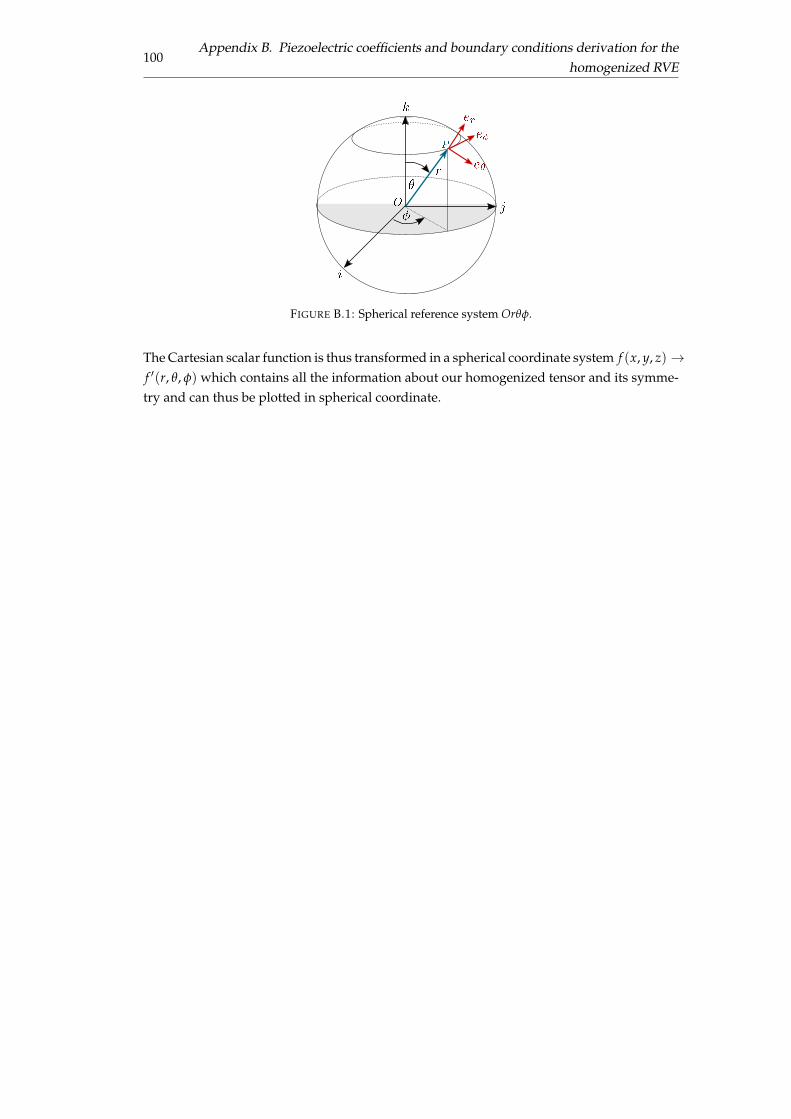
100Appendix B. Piezoelectric coefficients and boundary conditions derivation for the
homogenized RVE
FIGURE B.1: Spherical reference system Orqf.
The Cartesian scalar function is thus transformed in a spherical coordinate system f (x, y, z) !f 0(r, q, f) which contains all the information about our homogenized tensor and its symme-try and can thus be plotted in spherical coordinate.
101
Appendix C
Meshfree approximation method
C.1 Material characterization
The material properties involved in the electromechanical bulk enthalpy defined in Eq. (2.2.1)and (2.2.2) are characterized by specifying the material tensors, here we report all the tensorsinvolved in Voigt notation as they are implemented.
Elasticity tensor C
The fourth-order tensor C charcaterizing isotropic elasticity is given by
C =
2
666666664
Cl Ct Ct 0 0 0Ct Cl Ct 0 0 0Ct Ct Cl 0 0 00 0 0 Cs 0 00 0 0 0 Cs 00 0 0 0 0 Cs
3
777777775
, (C.1)
with Cl , Ct and Cs defined in 2D plain strain condition in terms of Young’s modulus Y andPoisson’s ratio n as
Cl =Y(1 � n)
(1 + n)(1 � 2n), Ct =
Yn
(1 + n)(1 � 2n), Cs =
Y2(1 + n)
. (C.2)
Dielectricity tensor k
The second-order isotropic dielectricity tensor is written in terms of dielectric permittivity e
as
k =
2
64e 0 00 e 00 0 e
3
75 , (C.3)
Flexoelectricity tensor µ
Flexoelectricity is characterized by the fourth-rank tensor mu. Ferroelectric perovskites intheir paraelectric phase belong to the cubic point group m3m with only three independentflexoelectric components[32], namely longitudinal µ` = µ11, transverse µt = µ12 and shearµs = µ44.
µ =
2
64µ11 0 0 µ12 0 0 µ12 0 0 0 µ44 0 0 0 µ44 0 0 00 µ12 0 0 µ11 0 0 µ12 0 µ44 0 0 0 0 0 0 0 µ44
0 0 µ12 0 0 µ12 0 0 µ11 0 0 0 µ44 0 0 0 µ44 0
3
75 ,
(C.4)
102 Appendix C. Meshfree approximation method
where
µiiii = µ` i = 1, 2, 3; (C.5a)
µijji = µt i = 1, 2, 3; such that i 6= j (C.5b)
µiijj = µijij = µs i = 1, 2, 3; such that i 6= j, (C.5c)
Gradient operators Bu and Bf
The gradient operators can be written as
Bu =
2
664
∂∂x 0 0 ∂
∂y 0 ∂∂z
0 ∂∂y 0 ∂
∂x∂∂z 0
0 0 ∂∂z 0 ∂
∂y∂
∂x
3
775 , (C.6)
andBf =
h∂
∂x∂
∂y∂∂z
i. (C.7)
Hessian operators Hu and Hf
Hu =
2
64
∂2
∂x2∂2
∂x∂y∂2
∂x∂z 0 0 0 0 0 0
0 0 0 ∂2
∂y∂x∂2
∂y2∂2
∂y∂z 0 0 0
0 0 0 0 0 0 ∂2
∂z∂x∂2
∂z∂y∂2
∂z2 .
...
...
∂2
∂y∂x∂2
∂y2∂2
∂y∂z∂2
∂z∂x∂2
∂z∂y∂2
∂z2 0 0 0∂2
∂x2∂2
∂x∂y∂2
∂x∂z 0 0 0 ∂2
∂z∂x∂2
∂z∂y∂2
∂z2
0 0 0 ∂2
∂x2∂2
∂x∂y∂2
∂x∂z∂2
∂y∂x∂2
∂y2∂2
∂y∂z
3
775 (C.8)
C.2 Derivation of the elastic torsion problem in cylindricalcoordinates
The displacement field for the elastic torsion problem in cylindrical coordinates is written as
8>>><
>>>:
ur = 0,
uq = a(z)rz,
uz = a(z)y(r, q, z).
(C.9)
C.3. Mesh and convergence 103
From here, the non-zero strain gradient components can be derived as reported below
#zz,z = a00y + 2a0∂y
∂z+ a
∂2y
∂z2 , (C.10a)
#zz,q =1r
✓a0
∂y
∂q+ a
∂2y
∂q∂z
◆, (C.10b)
#zz,r =1r
✓a0y + a
∂y
∂z
◆+ a0
∂y
∂r+ a
∂2y
∂r∂z, (C.10c)
#qz,z = #zq,z =12
✓a00rz + 2a0r +
1r
a0∂y
∂q+
1r
a∂2y
∂q∂z
◆, (C.10d)
#rz,z = #zr,z =a
2∂2y
∂r∂z, (C.10e)
#qz,q = #zq,q =a
2
✓1r
∂y
∂r+
∂2y
∂r2
◆, (C.10f)
where a0 = ∂a/∂z and a00 = ∂2a/∂z2.
C.3 Mesh and convergence
Axisymmetric structured meshes have been used in order to avoid mesh-dependent sym-metries. Figure C.1(a) shows the electric potential distribution on a quarter cross-sectionobtained from simulations with two different meshes, where the second one (right) has beenobtained upon rotation of the first one (left) by an angle z = 20. The observed patternsagree perfectly and bear no relation with the computational mesh, thereby discarding anynumerical artifact. Furthermore, the observed domain patterns are converged as illustratedin Figure C.1(b) showing that the electric potential distribution on a quarter cross-sectionis not affected by mesh refinement. All simulation results in the paper have been obtainedwith the finest mesh (right).
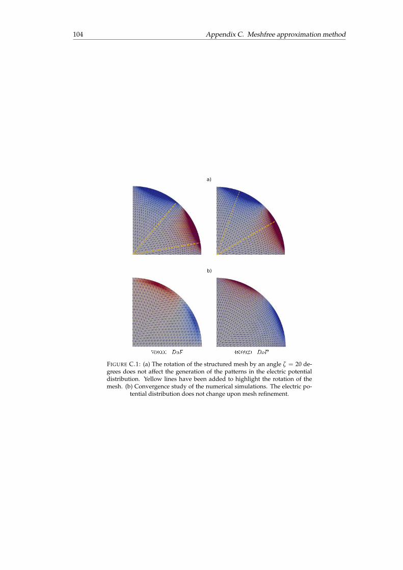
104 Appendix C. Meshfree approximation method
a)
b)
FIGURE C.1: (a) The rotation of the structured mesh by an angle z = 20 de-grees does not affect the generation of the patterns in the electric potentialdistribution. Yellow lines have been added to highlight the rotation of themesh. (b) Convergence study of the numerical simulations. The electric po-
tential distribution does not change upon mesh refinement.
105
Bibliography
[1] Canan Dagdeviren et al. “Recent progress in flexible and stretchable piezoelectric de-vices for mechanical energy harvesting, sensing and actuation”. In: Extreme mechanicsletters 9 (2016), pp. 269–281.
[2] Gustav Gautschi. “Piezoelectric sensors”. In: Piezoelectric Sensorics. Springer, 2002,pp. 73–91.
[3] Mohsen Safaei, Henry A Sodano, and Steven R Anton. “A review of energy har-vesting using piezoelectric materials: state-of-the-art a decade later (2008–2018)”. In:Smart Materials and Structures 28.11 (2019), p. 113001.
[4] Nipun Sinha et al. “Piezoelectric aluminum nitride nanoelectromechanical actua-tors”. In: Applied Physics Letters 95.5 (2009), p. 053106.
[5] Takuro Ikeda. Fundamentals of piezoelectricity. Oxford Science Publications. OxfordUniversity Press, 1997.
[6] Jürgen Rödel et al. “Perspective on the development of lead-free piezoceramics”. In:Journal of the American Ceramic Society 92.6 (2009), pp. 1153–1177.
[7] B Jaffe, RS Roth, and S Marzullo. “Properties of Piezoelectric Cerdmics in the Solid-Solution”. In: Journal of research of the National Bureau of Standards 55 (1955), p. 239.
[8] Eric Cross. “Lead-free at last”. In: Nature 432.7013 (2004), pp. 24–25.
[9] Chang-Hyo Hong et al. “Lead-free piezoceramics–Where to move on?” In: Journal ofMateriomics 2.1 (2016), pp. 1–24.
[10] Yasuyoshi Saito et al. “Lead-free piezoceramics”. In: Nature 432.7013 (2004), pp. 84–87.
[11] Jiagang Wu. “Perovskite lead-free piezoelectric ceramics”. In: Journal of Applied Physics127.19 (2020), p. 190901.
[12] V Sundar and RE Newnham. “Electrostriction and polarization”. In: Ferroelectrics135.1 (1992), pp. 431–446.
[13] David Codony. “Mathematical and computational modeling of flexoelectricity at meso-scopic and atomistic scales”. PhD thesis. Universitat Politècnica de Catalunya, 2021.
[14] VS Mashkevich and KB Tolpygo. “Electrical, optical and elastic properties of dia-mond type crystals”. In: Sov. Phys. JETP 5.3 (1957), pp. 435–439.
[15] Sh M Kogan. “Piezoelectric effect during inhomogeneous deformation and acousticscattering of carriers in crystals”. In: Soviet Physics-Solid State 5.10 (1964), pp. 2069–2070.
[16] EV Bursian and ZAIKOVSK. OI. “Changes in curvature of a ferroelectric film due topolarization”. In: Soviet Physics Solid State, USSR 10.5 (1968), pp. 1121–+.
106 BIBLIOGRAPHY
[17] Robert B Meyer. “Piezoelectric effects in liquid crystals”. In: Physical Review Letters22.18 (1969), p. 918.
[18] W Huang, F-G Yuan, and X Jiang. “Flexoelectric effect, materials, and structures”.In: Structural Health Monitoring (SHM) in Aerospace Structures. Elsevier, 2016, pp. 119–148.
[19] M Marvan and A Havránek. “Flexoelectric effect in elastomers”. In: Relationships ofPolymeric Structure and Properties. Springer, 1998, pp. 33–36.
[20] Qian Deng, Liping Liu, and Pradeep Sharma. “Flexoelectricity in soft materials andbiological membranes”. In: Journal of the Mechanics and Physics of Solids 62 (2014),pp. 209–227.
[21] Matthew Grasinger, Kosar Mozaffari, and Pradeep Sharma. “Flexoelectricity in softelastomers and the molecular mechanisms underpinning the design and emergenceof giant flexoelectricity”. In: Proceedings of the National Academy of Sciences 118.21(2021).
[22] Dennis S Bruhn, Michael A Lomholt, and Himanshu Khandelia. “Quantifying therelationship between curvature and electric potential in lipid bilayers”. In: The Journalof Physical Chemistry B 120.21 (2016), pp. 4812–4817.
[23] Haoyu Chen, Daniel Garcia-Gonzalez, and Antoine Jérusalem. “Computational modelof the mechanoelectrophysiological coupling in axons with application to neuromod-ulation”. In: Physical Review E 99.3 (2019), p. 032406.
[24] Kathryn D Breneman, William E Brownell, and Richard D Rabbitt. “Hair cell bundles:flexoelectric motors of the inner ear”. In: PLoS One 4.4 (2009), e5201.
[25] Elisabetta Sassaroli and Natalia Vykhodtseva. “Acoustic neuromodulation from a ba-sic science prospective”. In: Journal of therapeutic ultrasound 4.1 (2016), pp. 1–14.
[26] Fabian Vasquez-Sancho et al. “Flexoelectricity in bones”. In: Advanced materials 30.9(2018), p. 1705316.
[27] Pavlo Zubko, Gustau Catalan, and Alexander K Tagantsev. “Flexoelectric effect insolids”. In: Annual Review of Materials Research 43 (2013).
[28] P Ivaldi et al. “50 nm thick AlN film-based piezoelectric cantilevers for gravimetricdetection”. In: Journal of Micromechanics and Microengineering 21.8 (2011), p. 085023.
[29] Seok Ju Kang et al. “Printable ferroelectric PVDF/PMMA blend films with ultralowroughness for low voltage non-volatile polymer memory”. In: Advanced FunctionalMaterials 19.17 (2009), pp. 2812–2818.
[30] Amir Abdollahi and Irene Arias. “Constructive and destructive interplay betweenpiezoelectricity and flexoelectricity in flexural sensors and actuators”. In: Journal ofApplied Mechanics 82.12 (2015).
[31] Longlong Shu et al. “Symmetry of flexoelectric coefficients in crystalline medium”.In: Journal of Applied Physics 110.10 (2011), p. 104106.
[32] Longlong Shu et al. “Erratum:“Symmetry of flexoelectric coefficients in crystallinemedium”[J. Appl. Phys. 110, 104106 (2011)]”. In: Journal of Applied Physics 116.12(2014), p. 129901.
BIBLIOGRAPHY 107
[33] H Le Quang and Q-C He. “The number and types of all possible rotational sym-metries for flexoelectric tensors”. In: Proceedings of the Royal Society A: Mathematical,Physical and Engineering Sciences 467.2132 (2011), pp. 2369–2386.
[34] Amir Abdollahi et al. “Revisiting pyramid compression to quantify flexoelectricity:A three-dimensional simulation study”. In: Physical Review B 91.10 (2015), p. 104103.
[35] L Eric Cross. “Flexoelectric effects: Charge separation in insulating solids subjectedto elastic strain gradients”. In: Journal of Materials Science 41.1 (2006), pp. 53–63.
[36] Wenhui Ma and L Eric Cross. “Large flexoelectric polarization in ceramic lead mag-nesium niobate”. In: Applied Physics Letters 79.26 (2001), pp. 4420–4422.
[37] Wenhui Ma and L Eric Cross. “Flexoelectric polarization of barium strontium titanatein the paraelectric state”. In: Applied Physics Letters 81.18 (2002), pp. 3440–3442.
[38] Wenhui Ma and L Eric Cross. “Flexoelectric effect in ceramic lead zirconate titanate”.In: Applied Physics Letters 86.7 (2005), p. 072905.
[39] Wenhui Ma and L Eric Cross. “Flexoelectricity of barium titanate”. In: Applied PhysicsLetters 88.23 (2006), p. 232902.
[40] Amir Abdollahi et al. “Computational evaluation of the flexoelectric effect in dielec-tric solids”. In: Journal of Applied Physics 116.9 (2014), p. 093502.
[41] Wenyi Zhu et al. “Piezoelectric composite based on the enhanced flexoelectric ef-fects”. In: Applied physics letters 89.19 (2006), p. 192904.
[42] Umesh Kumar Bhaskar et al. “Flexoelectric MEMS: towards an electromechanicalstrain diode”. In: Nanoscale 8.3 (2016), pp. 1293–1298.
[43] Wenbin Huang et al. “Flexoelectric strain gradient detection using Ba0. 64Sr0. 36TiO3for sensing”. In: Applied Physics Letters 101.25 (2012), p. 252903.
[44] Victor Ishrayelu Merupo et al. “Flexoelectric response in soft polyurethane films andtheir use for large curvature sensing”. In: Journal of Applied Physics 122.14 (2017),p. 144101.
[45] X Yan et al. “Design of a curvature sensor using a flexoelectric material”. In: Sen-sors and Smart Structures Technologies for Civil, Mechanical, and Aerospace Systems 2013.Vol. 8692. International Society for Optics and Photonics. 2013, 86920N.
[46] Lu Qi et al. “On the mechanics of curved flexoelectric microbeams”. In: InternationalJournal of Engineering Science 124 (2018), pp. 1–15.
[47] Longlong Shu et al. “Flexoelectric materials and their related applications: A focusedreview”. In: Journal of Advanced Ceramics (2019), pp. 1–21.
[48] KF Wang and BL Wang. “Energy gathering performance of micro/nanoscale circularenergy harvesters based on flexoelectric effect”. In: Energy 149 (2018), pp. 597–606.
[49] Gustau Catalan et al. “Flexoelectric rotation of polarization in ferroelectric thin films”.In: Nature materials 10.12 (2011), pp. 963–967.
[50] Haidong Lu et al. “Mechanical writing of ferroelectric polarization”. In: Science 336.6077(2012), pp. 59–61.
[51] Sung Min Park et al. “Selective control of multiple ferroelectric switching pathwaysusing a trailing flexoelectric field”. In: Nature Nanotechnology 13.5 (2018), pp. 366–370.
108 BIBLIOGRAPHY
[52] Sana Krichen and Pradeep Sharma. “Flexoelectricity: A perspective on an unusualelectromechanical coupling”. In: Journal of Applied Mechanics 83.3 (2016).
[53] ND Sharma, Ravi Maranganti, and P Sharma. “On the possibility of piezoelectricnanocomposites without using piezoelectric materials”. In: Journal of the Mechanicsand Physics of Solids 55.11 (2007), pp. 2328–2350.
[54] Chang Liu, Huaping Wu, and Jie Wang. “Giant piezoelectric response in piezoelec-tric/dielectric superlattices due to flexoelectric effect”. In: Applied Physics Letters 109.19(2016), p. 192901.
[55] Qian Deng et al. “Nanoscale flexoelectric energy harvesting”. In: International Journalof Solids and Structures 51.18 (2014), pp. 3218–3225.
[56] J Fousek, LE Cross, and DB Litvin. “Possible piezoelectric composites based on theflexoelectric effect”. In: Materials Letters 39.5 (1999), pp. 287–291.
[57] John Y Fu et al. “Gradient scaling phenomenon in microsize flexoelectric piezoelectriccomposites”. In: Applied Physics Letters 91.18 (2007), p. 182910.
[58] Baojin Chu et al. “Flexure mode flexoelectric piezoelectric composites”. In: Journal ofApplied Physics 106.10 (2009), p. 104109.
[59] David Codony et al. “An Immersed Boundary Hierarchical B-spline method for flex-oelectricity”. In: Computer Methods in Applied Mechanics and Engineering 354 (2019),pp. 750–782.
[60] Alice Mocci et al. “Geometrically polarized architected dielectrics with effective piezo-electricity”. In: Submitted for publication (2021).
[61] Alice Mocci, Prakhar Gupta, and Irene Arias. “Shape optimization of architected di-electrics with effective piezoelectricity using computational homogenization”. In: Inpreparation (2021).
[62] Alice Mocci, Amir Abdollahi, and Irene Arias. “Flexoelectricity in dielectrics undertorsion.” In: Submitted for publication (2020).
[63] Alice Mocci, Amir Abdollahi, and Irene Arias. “Flexoelectric bars under torsion: chas-ing the elusive shear flexoelectricity.” In: To be submitted (2021).
[64] David Codony et al. “Wheel-shaped and helical torsional flexoelectric devices”. In:In preparation (2021).
[65] Jordi Barceló-Mercader et al. “Generalized periodicity conditions for the computa-tional modeling of flexoelectric metamaterials”. In: Submitted for publication (2021).
[66] Raymond David Mindlin and NN Eshel. “On first strain-gradient theories in linearelasticity”. In: International Journal of Solids and Structures 4.1 (1968), pp. 109–124.
[67] AK Tagantsev. “Piezoelectricity and flexoelectricity in crystalline dielectrics”. In: Phys-ical Review B 34.8 (1986), p. 5883.
[68] Alexander K Tagantsev. “Electric polarization in crystals and its response to thermaland elastic perturbations”. In: Phase Transitions: A Multinational Journal 35.3-4 (1991),pp. 119–203.
[69] PV Yudin and AK Tagantsev. “Fundamentals of flexoelectricity in solids”. In: Nan-otechnology 24.43 (2013), p. 432001.
BIBLIOGRAPHY 109
[70] Thanh D Nguyen et al. “Nanoscale flexoelectricity”. In: Advanced Materials 25.7 (2013),pp. 946–974.
[71] MS Majdoub, P Sharma, and T Cagin. “Enhanced size-dependent piezoelectricity andelasticity in nanostructures due to the flexoelectric effect”. In: Physical Review B 77.12(2008), p. 125424.
[72] MS Majdoub, P Sharma, and T Çagin. “Erratum: Enhanced size-dependent piezoelec-tricity and elasticity in nanostructures due to the flexoelectric effect [Phys. Rev. B 77,125424 (2008)]”. In: Physical Review B 79.11 (2009), p. 119904.
[73] P Zubko et al. “Strain-gradient-induced polarization in SrTiO 3 single crystals”. In:Physical Review Letters 99.16 (2007), p. 167601.
[74] Amir Abdollahi et al. “Fracture toughening and toughness asymmetry induced byflexoelectricity”. In: Physical Review B 92.9 (2015), p. 094101.
[75] Xiaoying Zhuang et al. “Computational modeling of flexoelectricity—a review”. In:Energies 13.6 (2020), p. 1326.
[76] E Amanatidou and N Aravas. “Mixed finite element formulations of strain-gradientelasticity problems”. In: Computer Methods in Applied Mechanics and Engineering 191.15-16 (2002), pp. 1723–1751.
[77] John Y Shu, Wayne E King, and Norman A Fleck. “Finite elements for materials withstrain gradient effects”. In: International Journal for Numerical Methods in Engineering44.3 (1999), pp. 373–391.
[78] Sheng Mao, Prashant K Purohit, and Nikolaos Aravas. “Mixed finite-element formu-lations in piezoelectricity and flexoelectricity”. In: Proceedings of the Royal Society A:Mathematical, Physical and Engineering Sciences 472.2190 (2016), p. 20150879.
[79] Hamid Ghasemi, Harold S Park, and Timon Rabczuk. “A level-set based IGA formu-lation for topology optimization of flexoelectric materials”. In: Computer Methods inApplied Mechanics and Engineering 313 (2017), pp. 239–258.
[80] BH Nguyen, X Zhuang, and Timon Rabczuk. “NURBS-based formulation for non-linear electro-gradient elasticity in semiconductors”. In: Computer Methods in AppliedMechanics and Engineering 346 (2019), pp. 1074–1095.
[81] Carl De Boor and Carl De Boor. A practical guide to splines. Vol. 27. springer-verlagNew York, 1978.
[82] Charles S Peskin. “The immersed boundary method”. In: Acta numerica 11 (2002),pp. 479–517.
[83] Rajat Mittal and Gianluca Iaccarino. “Immersed boundary methods”. In: Annu. Rev.Fluid Mech. 37 (2005), pp. 239–261.
[84] Freddie D Witherden and Peter E Vincent. “On the identification of symmetric quadra-ture rules for finite element methods”. In: Computers & Mathematics with Applications69.10 (2015), pp. 1232–1241.
[85] William E Lorensen and Harvey E Cline. “Marching cubes: A high resolution 3D sur-face construction algorithm”. In: ACM siggraph computer graphics 21.4 (1987), pp. 163–169.
110 BIBLIOGRAPHY
[86] Onofre Marco et al. “Exact 3D boundary representation in finite element analysisbased on Cartesian grids independent of the geometry”. In: International Journal forNumerical Methods in Engineering 103.6 (2015), pp. 445–468.
[87] Ruben Sevilla, Sonia Fernández-Méndez, and Antonio Huerta. “NURBS-enhancedfinite element method (NEFEM)”. In: International Journal for Numerical Methods inEngineering 76.1 (2008), pp. 56–83.
[88] Ruben Sevilla and Sonia Fernández-Méndez. “Numerical integration over 2D NURBS-shaped domains with applications to NURBS-enhanced FEM”. In: Finite Elements inAnalysis and Design 47.10 (2011), pp. 1209–1220.
[89] Klaus Höllig, Jörg Hörner, and Axel Hoffacker. “Finite element analysis with B-splines:weighted and isogeometric methods”. In: International Conference on Curves and Sur-faces. Springer. 2010, pp. 330–350.
[90] Marino Arroyo and Michael Ortiz. “Local maximum-entropy approximation schemes:a seamless bridge between finite elements and meshfree methods”. In: Internationaljournal for numerical methods in engineering 65.13 (2006), pp. 2167–2202.
[91] Marino Arroyo and Michael Ortiz. “Local maximum-entropy approximation schemes”.In: Meshfree methods for partial differential equations III. Springer, 2007, pp. 1–16.
[92] Adrian Rosolen, Daniel Millán, and Marino Arroyo. “On the optimum support sizein meshfree methods: a variational adaptivity approach with maximum-entropy ap-proximants”. In: International Journal for Numerical Methods in Engineering 82.7 (2010),pp. 868–895.
[93] Victor Georgievich Veselago. “The Electrodynamics of Substances with Simultane-ously Negative Values of # and µ”. In: Physics-Uspekhi 10.4 (1968), pp. 509–514.
[94] Tie Jun Cui, David R Smith, and Ruopeng Liu. Metamaterials. Springer, 2010.
[95] Richard A Shelby, David R Smith, and Seldon Schultz. “Experimental verification ofa negative index of refraction”. In: science 292.5514 (2001), pp. 77–79.
[96] Richard W Ziolkowski. “Metamaterial-inspired efficient electrically-small antennas:Designs and experiments”. In: 2007 International Workshop on Anti-Counterfeiting, Se-curity and Identification (ASID). IEEE. 2007, pp. 4–4.
[97] Xiang Liu, Guoping Cai, and KW Wang. “Synthesizing and reconfiguring metastablemodular metamaterials for adaptive wave propagation control”. In: Journal of Soundand Vibration 468 (2020), p. 115114.
[98] YY Chen and GL Huang. “Active elastic metamaterials for subwavelength wavepropagation control”. In: Acta Mechanica Sinica 31.3 (2015), pp. 349–363.
[99] Vladimir M Shalaev. “Optical negative-index metamaterials”. In: Nature photonics 1.1(2007), pp. 41–48.
[100] Steven A Cummer, Johan Christensen, and Andrea Alù. “Controlling sound withacoustic metamaterials”. In: Nature Reviews Materials 1.3 (2016), pp. 1–13.
[101] Xiaoyu Zheng et al. “Ultralight, ultrastiff mechanical metamaterials”. In: Science 344.6190(2014), pp. 1373–1377.
[102] Lucas R Meza, Satyajit Das, and Julia R Greer. “Strong, lightweight, and recoverablethree-dimensional ceramic nanolattices”. In: Science 345.6202 (2014), pp. 1322–1326.
BIBLIOGRAPHY 111
[103] Katia Bertoldi et al. “Flexible mechanical metamaterials”. In: Nature Reviews Materials2.11 (2017), pp. 1–11.
[104] Sahab Babaee et al. “3D soft metamaterials with negative Poisson’s ratio”. In: Ad-vanced Materials 25.36 (2013), pp. 5044–5049.
[105] H Coufal and A Mandelis. “Pyroelectric sensors for the photothermal analysis of con-densed phases”. In: Ferroelectrics 118.1 (1991), pp. 379–409.
[106] Zhi Yan. “Modeling of a piezoelectric/piezomagnetic nano energy harvester basedon two dimensional theory”. In: Smart Materials and Structures 27.1 (2017), p. 015016.
[107] Kenji Uchino. Ferroelectric devices. CRC press, 2018.
[108] Walter Heywang, Karl Lubitz, and Wolfram Wersing. Piezoelectricity: evolution andfuture of a technology. Vol. 114. Springer Science & Business Media, 2008.
[109] Gene H Haertling. “Ferroelectric ceramics: history and technology”. In: Journal of theAmerican Ceramic Society 82.4 (1999), pp. 797–818.
[110] Bernard Jaffe. Piezoelectric ceramics. Vol. 3. Elsevier, 2012.
[111] Thomas R Shrout et al. “High performance, high temperature perovskite piezoelectrics”.In: 14th IEEE International Symposium on Applications of Ferroelectrics, 2004. ISAF-04.2004. IEEE. 2004, pp. 126–129.
[112] Roderic Lakes. “Elastic and viscoelastic behavior of chiral materials”. In: Internationaljournal of mechanical sciences 43.7 (2001), pp. 1579–1589.
[113] Alberto Biancoli et al. “Breaking of macroscopic centric symmetry in paraelectricphases of ferroelectric materials and implications for flexoelectricity”. In: Nature ma-terials 14.2 (2015), pp. 224–229.
[114] Walter Guyton Cady. Piezoelectricity: Volume Two: An Introduction to the Theory andApplications of Electromechanical Phenomena in Crystals. Courier Dover Publications,2018.
[115] Shashank Priya. “Advances in energy harvesting using low profile piezoelectric trans-ducers”. In: Journal of electroceramics 19.1 (2007), pp. 167–184.
[116] Swapnil Chandratre and Pradeep Sharma. “Coaxing graphene to be piezoelectric”.In: Applied Physics Letters 100.2 (2012), p. 023114.
[117] Jordi Barceló-Mercader et al. “Nitsche’s method for interfaces in flexoelectricity andapplication to periodic structures”. In: Submitted for publication (2021).
[118] Sheng Mao and Prashant K Purohit. “Insights into flexoelectric solids from strain-gradient elasticity”. In: Journal of Applied Mechanics 81.8 (2014).
[119] Dongchan Jang et al. “Fabrication and deformation of three-dimensional hollow ce-ramic nanostructures”. In: Nature materials 12.10 (2013), pp. 893–898.
[120] Yanling Gao et al. “Nanocrystalline barium strontium titanate ceramics synthesizedvia the “organosol” route and spark plasma sintering”. In: Journal of the AmericanCeramic Society 97.7 (2014), pp. 2139–2146.
[121] Bo Wang et al. “Flexoelectricity in solids: Progress, challenges, and perspectives”. In:Progress in Materials Science 106 (2019), p. 100570.
[122] John Y Fu et al. “Experimental studies of the converse flexoelectric effect induced byinhomogeneous electric field in a barium strontium titanate composition”. In: Journalof Applied Physics 100.2 (2006), p. 024112.
112 BIBLIOGRAPHY
[123] R Maranganti and P Sharma. “Length scales at which classical elasticity breaks downfor various materials”. In: Physical review letters 98.19 (2007), p. 195504.
[124] P Hana. “Study of flexoelectric phenomenon from direct and from inverse flexoelec-tric behavior of PMNT ceramic”. In: Ferroelectrics 351.1 (2007), pp. 196–203.
[125] VS Deshpande, MF Ashby, and NA Fleck. “Foam topology: bending versus stretch-ing dominated architectures”. In: Acta materialia 49.6 (2001), pp. 1035–1040.
[126] Christopher M Spadaccini. “Additive manufacturing and processing of architectedmaterials”. In: MRS Bulletin 44.10 (2019), pp. 782–788.
[127] John H Conway and Daniel H Huson. “The orbifold notation for two-dimensionalgroups”. In: Structural Chemistry 13.3 (2002), pp. 247–257.
[128] AL Kholkin et al. “Piezoelectric and electrostrictive ceramics transducers and actu-ators: Smart ferroelectric ceramics for transducer applications”. In: Smart Materials.CRC Press, 2008, pp. 9–1.
[129] Sarah Guerin and Damien Thompson. “Restriction boosts piezoelectricity”. In: NatureMaterials (2021), pp. 1–2.
[130] Muamer Kadic et al. “3D metamaterials”. In: Nature Reviews Physics 1.3 (2019), pp. 198–210.
[131] Alexander K. Tagantsev and Alexander S. Yurkov. “Flexoelectric effect in finite sam-ples”. In: Journal of Applied Physics 112.4 (2012), p. 044103. DOI: 10.1063/1.4745037.eprint: http://dx.doi.org/10.1063/1.4745037. URL: http://dx.doi.org/10.1063/1.4745037.
[132] Julien Yvonnet, Xing Chen, and Pradeep Sharma. “Apparent flexoelectricity due toheterogeneous piezoelectricity”. In: Journal of Applied Mechanics 87.11 (2020).
[133] Xin Wen et al. “Flexoelectret: an electret with a tunable flexoelectriclike response”. In:Physical review letters 122.14 (2019), p. 148001.
[134] Xin Wen et al. “Inverse flexoelectret effect: bending dielectrics by a uniform electricfield”. In: Physical Review Applied 15.1 (2021), p. 014032.
[135] Martin Philip Bendsoe and Ole Sigmund. Topology optimization: theory, methods, andapplications. Springer Science & Business Media, 2013.
[136] Lucas R Meza et al. “Resilient 3D hierarchical architected metamaterials”. In: Proceed-ings of the National Academy of Sciences 112.37 (2015), pp. 11502–11507.
[137] Michel Bornert. Homogenization in mechanics of materials. ISTE USA, 2008.
[138] George Dvorak. Micromechanics of composite materials. Vol. 186. Springer Science &Business Media, 2012.
[139] D Guinovart-Sanjuán et al. “Effective predictions of heterogeneous flexoelectric mul-tilayered composite with generalized periodicity”. In: International Journal of Mechan-ical Sciences 181 (2020), p. 105755.
[140] Donald F Adams and Douglas R Doner. “Transverse normal loading of a unidirec-tional composite”. In: Journal of composite Materials 1.2 (1967), pp. 152–164.
[141] Marc GD Geers, Varvara G Kouznetsova, and WAM Brekelmans. “Multi-scale com-putational homogenization: Trends and challenges”. In: Journal of computational andapplied mathematics 234.7 (2010), pp. 2175–2182.
BIBLIOGRAPHY 113
[142] BA Le, Julien Yvonnet, and Q-C He. “Computational homogenization of nonlinearelastic materials using neural networks”. In: International Journal for Numerical Meth-ods in Engineering 104.12 (2015), pp. 1061–1084.
[143] EWC Coenen et al. “A multi-scale approach to bridge microscale damage and macroscalefailure: a nested computational homogenization-localization framework”. In: Interna-tional journal of fracture 178.1-2 (2012), pp. 157–178.
[144] H Berger et al. “Finite element and asymptotic homogenization methods applied tosmart composite materials”. In: Computational mechanics 33.1 (2003), pp. 61–67.
[145] Harald Berger et al. “An analytical and numerical approach for calculating effec-tive material coefficients of piezoelectric fiber composites”. In: International Journalof Solids and Structures 42.21-22 (2005), pp. 5692–5714.
[146] Julien Yvonnet. Computational homogenization of heterogeneous materials with finite ele-ments. Springer, 2019.
[147] Rodney Hill. “Elastic properties of reinforced solids: some theoretical principles”. In:Journal of the Mechanics and Physics of Solids 11.5 (1963), pp. 357–372.
[148] Rodney Hill. “The essential structure of constitutive laws for metal composites andpolycrystals”. In: Journal of the Mechanics and Physics of Solids 15.2 (1967), pp. 79–95.
[149] Q-C He and Q-S Zheng. “On the symmetries of 2D elastic and hyperelastic tensors”.In: Journal of elasticity 43.3 (1996), pp. 203–225.
[150] Sten Haastrup et al. “The Computational 2D Materials Database: high-throughputmodeling and discovery of atomically thin crystals”. In: 2D Materials 5.4 (2018), p. 042002.
[151] Houssam Abdoul-Anziz, Nicolas Auffray, and Boris Desmorat. “Symmetry Classesand Matrix Representations of the 2D Flexoelectric Law”. In: Symmetry 12.4 (2020),p. 674.
[152] Stefan J Rupitsch. Piezoelectric sensors and actuators. Springer, 2019.
[153] Mohammad H Malakooti and Henry A Sodano. “Piezoelectric energy harvestingthrough shear mode operation”. In: Smart Materials and Structures 24.5 (2015), p. 055005.
[154] Dung-An Wang and Nine-Zeng Liu. “A shear mode piezoelectric energy harvesterbased on a pressurized water flow”. In: Sensors and actuators A: Physical 167.2 (2011),pp. 449–458.
[155] Jihe Zhao et al. “Investigation of a d15 mode PZT-51 piezoelectric energy harvesterwith a series connection structure”. In: Smart materials and structures 21.10 (2012),p. 105006.
[156] Henry A Sodano, Gyuhae Park, and DJ Inman. “Estimation of electric charge outputfor piezoelectric energy harvesting”. In: Strain 40.2 (2004), pp. 49–58.
[157] ND Sharma, CM Landis, and P Sharma. “Piezoelectric thin-film superlattices withoutusing piezoelectric materials”. In: Journal of Applied Physics 108.2 (2010), p. 024304.
[158] Jorge Nocedal and Stephen Wright. Numerical optimization. Springer Science & Busi-ness Media, 2006.
[159] NA Fleck et al. “Strain gradient plasticity: theory and experiment”. In: Acta Metallur-gica et materialia 42.2 (1994), pp. 475–487.
114 BIBLIOGRAPHY
[160] Y Huang et al. “Mechanism-based strain gradient plasticity—II. Analysis”. In: Journalof the Mechanics and Physics of Solids 48.1 (2000), pp. 99–128.
[161] ACM Chong et al. “Torsion and bending of micron-scaled structures”. In: Journal ofMaterials Research 16.4 (2001), pp. 1052–1058.
[162] KA Lazopoulos and AK Lazopoulos. “On the torsion problem of strain gradient elas-tic bars”. In: Mechanics Research Communications 45 (2012), pp. 42–47.
[163] Shuwen Zhang et al. “Shear flexoelectric response along 3121 direction in polyvinyli-dene fluoride”. In: Applied Physics Letters 107.14 (2015), p. 142902.
[164] Shuwen Zhang et al. “Investigation of the 2312 flexoelectric coefficient componentof polyvinylidene fluoride: Deduction, simulation, and mensuration”. In: Scientificreports 7.1 (2017), pp. 1–9.
[165] Alexander K Tagantsev, Eric Courtens, and Ludovic Arzel. “Prediction of a low-temperature ferroelectric instability in antiphase domain boundaries of strontium ti-tanate”. In: Physical Review B 64.22 (2001), p. 224107.
[166] Longlong Shu et al. “Converse flexoelectric coefficient f 1212 in bulk Ba0. 67Sr0.33TiO3”. In: Applied Physics Letters 104.23 (2014), p. 232902.
[167] Kaiyuan Liu et al. “Experimental decoupling of cylindrical flexoelectric coefficients”.In: Applied Physics Letters 113.10 (2018), p. 102902.
[168] Kaiyuan Liu et al. “Decoupled shear flexoelectric effects in polymers”. In: Journal ofApplied Physics 125.17 (2019), p. 174104.
[169] IS Sokolnikoff. “Mathematical theory of elasticity”. In: Bull. Amer. Math. Soc 52 (1946),pp. 976–978.
[170] Robert Asaro and Vlado Lubarda. Mechanics of solids and materials. Cambridge Uni-versity Press, 2006.
[171] Z Yan and LY Jiang. “Flexoelectric effect on the electroelastic responses of bendingpiezoelectric nanobeams”. In: Journal of Applied Physics 113.19 (2013), p. 194102.
[172] Xu Liang, Shuling Hu, and Shengping Shen. “Effects of surface and flexoelectricityon a piezoelectric nanobeam”. In: Smart materials and structures 23.3 (2014), p. 035020.
[173] Runzhi Zhang, Xu Liang, and Shengping Shen. “A Timoshenko dielectric beam modelwith flexoelectric effect”. In: Meccanica 51.5 (2016), pp. 1181–1188.
[174] J. Francu and P. Novácková P. ans Janícek. “Torsion of non circular bar”. In: Engi-neering Mechanics, Vol. 19 (2012). URL: http://www.kmp.tul.cz/system/files/krouceni_nekruhoveho_hridele_francu.pdf.
[175] Johannes Tesse Bastiaan Overvelde, Sicong Shan, and Katia Bertoldi. “Compactionthrough buckling in 2D periodic, soft and porous structures: effect of pore shape”. In:Advanced Materials 24.17 (2012), pp. 2337–2342.
[176] HW Yap, RS Lakes, and Robert W Carpick. “Negative stiffness and enhanced damp-ing of individual multiwalled carbon nanotubes”. In: Physical Review B 77.4 (2008),p. 045423.
[177] Raymond David Mindlin. Microstructure in linear elasticity. Tech. rep. Columbia UnivNew York Dept of Civil Engineering and Engineering Mechanics, 1963.

BIBLIOGRAPHY 115
[178] BS Altan and EC Aifantis. “On some aspects in the special theory of gradient elastic-ity”. In: Journal of the Mechanical Behavior of Materials 8.3 (1997), pp. 231–282.
[179] A Cemal Eringen and DGB Edelen. “On nonlocal elasticity”. In: International journalof engineering science 10.3 (1972), pp. 233–248.
[180] Janusz Dyszlewicz. Micropolar theory of elasticity. Vol. 15. Springer Science & BusinessMedia, 2012.
[181] Yanmei Yue, Kaiyu Xu, and Elias C Aifantis. “Strain gradient and electric field gradi-ent effects in piezoelectric cantilever beams”. In: Journal of the Mechanical Behavior ofMaterials 24.3-4 (2015), pp. 121–127.