
Numerical modeling of anisotropic granular media
154
NUMERICAL MODELING OF ANISOTROPIC GRANULAR MEDIA Takeichi Kanzaki Cabrera Dipòsit legal: Gi. 899-2014 http://hdl.handle.net/10803/133834 http://creativecommons.org/licenses/by/4.0/deed.ca Aquesta obra està subjecta a una llicència Creative Commons Reconeixement Esta obra está bajo una licencia Creative Commons Reconocimiento This work is licensed under a Creative Commons Attribution licence
Transcript of Numerical modeling of anisotropic granular media

NUMERICAL MODELING OF ANISOTROPIC GRANULAR MEDIA
Takeichi Kanzaki Cabrera
Dipòsit legal: Gi. 899-2014 http://hdl.handle.net/10803/133834
http://creativecommons.org/licenses/by/4.0/deed.ca Aquesta obra està subjecta a una llicència Creative Commons Reconeixement Esta obra está bajo una licencia Creative Commons Reconocimiento This work is licensed under a Creative Commons Attribution licence
Universitat de Girona
Numerical modeling of anisotropic
granular media
PhD thesisby
Takeichi Kanzaki Cabrera
2013


Universitat de Girona
PhD thesis
Numerical modeling of anisotropic
granular media
Takeichi Kanzaki Cabrera
2013
Doctoral Programme in Technology
Thesis supervisors
Dr. Raúl Cruz Hidalgo Dr. Jordi Farjas Silva
University of Navarra, Spain Universitat de Girona, Spain
Report submitted to qualify for the PhD degree at the Universitat de Girona


To whom it might concern,
Dr. Raúl Cruz Hidalgo, Profesor Titular del Departamento de Física y Matemática
Aplicada Universidad de Navarra.
Dr. Jordi Farjas Silva, Profesor Titular del Departament de Física de la Univer-
sitat de Girona.
CERTIFY that the study entitled “Numerical modeling of anisotropic granu-
lar media“ has been carried out under their supervision by Takeichi Kanzaki
Cabrera to obtain the PhD degree, and accomplishes all the requirements to
be considered for the International Mention.
Girona, June 2013
Dr. Raúl Cruz Hidalgo Dr. Jordi Farjas Silva
University of Navarra, Spain Universitat de Girona, Spain


A ti,
que me has hecho todo lo que soy


The Spanish Government (Ministerio de Ciencia e Innovación) under re-
search grant FIS2008-06034-C02-01/02 and the Universitat de Girona (PhD
Fellowship Program) have supported this work.
The research stay of the author at the University of Twente has been founded
by the Universitat de Girona (Movability Research Stay Program).
Acknowledgements - Agradecimientos
First of all I would like to say thanks to my supervisors, Dr. Raúl Cruz Hi-
dalgo and Dr. Jordi Farjas Silva. Thanks for giving me this opportunity, for all
the advices and for the time you devoted to me.
I would like to acknowledge the Department of Physics of the Universitat de
Girona, and particularity to the research groups "Grup de Recerca en Ma-
terials i Termodinàmica" and "Analysis of Advanced Materials for Structural
Design (AMADE)".
I would also like to thank the research group "Multi Scale Mechanics (MSM)"
of the University of Twente, and specially to Professor Stefan Luding, Sebas-
tian Gonzalez and Fabian Uhlig for their support and interesting discussions
during my research stay at the University of Twente.
Professors Diego Maza, Iker Zuriguel, Ignacio Pagonabarraga and Fernando
Alonso-Marroquin has also made a great contribution to this work with their
wise advices and helpful professional exchanges.
There are many people to whom I owe a lot, without you it would have been
impossible to finish this work, many thanks to you all.
Als colegues d’AMADE, moltes gràcies per el vostre suport, per donar-me la
benvinguda a casa vostra, per els anys compartits, per les discussions a la
sobre taula, per els partits de futbol jugats.

A mi mamá, sin ti nada de esto hubiera pasado, muchas gracias por inten-
tar educarme, que no te lo he puesto nada fácil, por enseñarme que hay que
luchar por lo que uno quiere, y por los que uno quiere, por estar siempre ahí,
simplemente, GRACIAS.
A la meva dona, per tot el suport que m’has donat, per estar al meu co-
stat, per no donar-me treva els dies que no reaccionava, t’estimo amor.
A la vertiente cubana de mi familia, mi abuela, tío, tías, primos, mi papá,
hermanas, mi familia es un dibujo, pero es mi dibujo. Al vessant català de la
familia, moltes gràcies per fer-me sentir com a casa, per mitigar la sensació
de no tenir l’altra part de la familia a prop.
A mis amigos, a los de verdad, a los que siempre estuvieron ahí, cuando
los momentos no eran tan buenos, i encara hi són. A Raúl, sin ti no estaría
aquí, a Carmen, Tatá, Claudia, M.J., mi pequeña familia al llegar.
Una vez más, a mis dos mujeres, mis bastones, mis dos amores,
mis dos niñas.

List of Published papers
As a result of the present work there have been published the following pa-
pers:
• Pagonabarraga, I.; Kanzaki, T.; Hidalgo, R.C. The European Physical
Journal Special Topics, 179, pp.43-53 (2009) doi:10.1140/epjst/e2010-
01193-3
• Kanzaki, T.; Hidalgo, R.C.; Maza, D.; Pagonabarraga, I. "Cooling dynam-
ics of a granular gas of elongated". J. Stat. Mech. 2010 (2010) P06020
doi:10.1088/1742-5468/2010/06/P06020
• Kanzaki, T; M. Acevedo, I. Zuriguel, I. Pagonabarraga, D. Maza, R. C.
Hidalgo "Stress distribution of faceted particles in a silo after its partial
discharge" Eur. Phys. J. E 34 133 (2011) doi:10.1140/epje/i2011-11133-5
• R.C. Hidalgo, D. Kadau, T. Kanzaki and H. J. Herrmann "Granular pack-
ings of cohesive elongated particles" Granular Matter 14 191-196 (2012)
doi:10.1007/s10035-011-0303-2
• R.C. Hidalgo; Kanzaki, T; F. Alonso-Marroquin and S. Luding "On the
use of graphics processing units (GPUs) for molecular dynamics sim-
ulation of spherical particles" Powders & Grains 2013 169-172 (2013)
doi:http://dx.doi.org/10.1063/1.4811894

List of Figures
1.1 Interaction of two particles . . . . . . . . . . . . . . . . . . . . . . 10
1.2 Wall effect in MD simulations . . . . . . . . . . . . . . . . . . . . . 14
1.3 Periodic boundary condition . . . . . . . . . . . . . . . . . . . . . . 15
1.4 Heterogeneous programming model . . . . . . . . . . . . . . . . . 17
1.5 CPU and GPU Architecture . . . . . . . . . . . . . . . . . . . . . . 19
1.6 Evolution of FLOP . . . . . . . . . . . . . . . . . . . . . . . . . . . . 20
1.7 CUDA Heterogeneous Programming Model . . . . . . . . . . . . . 21
2.1 Time evolution of the particle size densities . . . . . . . . . . . . . 28
2.2 Scaled fragment size distribution (symmetric product kernels) . . 30
2.3 Scaled fragment size distribution (symmetric sum kernels) . . . . 31
2.4 Evolution of the normalized cumulative size density . . . . . . . . 32
2.5 Fragment size distribution . . . . . . . . . . . . . . . . . . . . . . . 34
2.6 Normalized cumulative size density (asymmetric sum kernels) . . 35
2.7 Normalized cumulative size density (asymmetric product kernels) 36
2.8 Scaled fragment size distribution (asymmetric product kernel) . . 37
3.1 Particles interaction . . . . . . . . . . . . . . . . . . . . . . . . . . 43
3.2 Periodic boundary conditions . . . . . . . . . . . . . . . . . . . . . 46
3.3 Spatial evolution of a system with γN = 1s−1 . . . . . . . . . . . . 48
3.4 Spatial evolution of a system with γN = 103s−1 . . . . . . . . . . . 49
3.5 Evolution of the translational kinetic energy . . . . . . . . . . . . 50
3.6 Evolution of the rotational kinetic energy . . . . . . . . . . . . . . 51
3.7 Scaled speed distribution . . . . . . . . . . . . . . . . . . . . . . . 53
3.8 Radial distribution function . . . . . . . . . . . . . . . . . . . . . . 55
3.9 Radial orientation distribution functions . . . . . . . . . . . . . . . 55
i

ii
3.10Nematic parameter . . . . . . . . . . . . . . . . . . . . . . . . . . . 57
4.1 Photograph of the experimental setup . . . . . . . . . . . . . . . . 60
4.2 Packings of square nuts and simulated particles . . . . . . . . . . 64
4.3 Experimental and numerical orientation distributions . . . . . . . 65
4.4 Experimental and numerical orientation of the squares . . . . . . 67
4.5 Polar distribution of the principal directions of the local stress . . 69
4.6 Trace of the mean stress tensor after the silo loading . . . . . . . 70
4.7 Trace of the mean stress tensor after the load for rods . . . . . . . 71
4.8 Trace of the mean stress tensor after the load for squares . . . . . 72
5.1 Simulated packings of elongated cohesive particles . . . . . . . . 76
5.2 Density profiles of different granular deposits . . . . . . . . . . . . 79
5.3 Orientation distributions of particles for two aspect ratios . . . . 80
5.4 Radial orientation distribution functions, Q(r) . . . . . . . . . . . 82
5.5 Polar distribution of the principal direction . . . . . . . . . . . . . 82
5.6 Profiles of the trace of the mean stress tensor . . . . . . . . . . . . 84
6.1 Cundall number behavior on CPU and GPU . . . . . . . . . . . . . 89
6.2 Two bodies interaction . . . . . . . . . . . . . . . . . . . . . . . . . 91
6.3 Flowchart of the granular gas simulation . . . . . . . . . . . . . . 94
6.4 Comparison of numerical with theoretical results . . . . . . . . . . 98
6.5 Scaled linear speed distribution . . . . . . . . . . . . . . . . . . . . 99
6.6 Scaled angular speed distribution . . . . . . . . . . . . . . . . . . 99
6.7 Cundall number behavior for different number of GPU . . . . . . . 101

Contents
Summary v
1 Introduction 1
1.1 Computational Physics . . . . . . . . . . . . . . . . . . . . . . . . . 2
1.1.1 Monte Carlo method . . . . . . . . . . . . . . . . . . . . . . 3
1.1.2 Molecular Dynamics . . . . . . . . . . . . . . . . . . . . . . . 5
1.2 Scientific programming . . . . . . . . . . . . . . . . . . . . . . . . 16
2 Collision induced fragmentation: a simple numerical algorithm 23
2.1 Mean Field Theory . . . . . . . . . . . . . . . . . . . . . . . . . . . 24
2.2 Direct Simulation Monte Carlo Algorithm . . . . . . . . . . . . . . 25
2.3 Symmetric Kernels . . . . . . . . . . . . . . . . . . . . . . . . . . . 28
2.3.1 Symmetric Deterministic Fragmentation . . . . . . . . . . . 28
2.3.2 Symmetric Stochastic Fragmentation . . . . . . . . . . . . . 29
2.4 Asymmetric Kernels . . . . . . . . . . . . . . . . . . . . . . . . . . 31
2.4.1 Asymmetric Deterministic Fragmentation . . . . . . . . . . 31
2.4.2 Asymmetric Stochastic Fragmentation . . . . . . . . . . . . 35
2.5 Discussion . . . . . . . . . . . . . . . . . . . . . . . . . . . . . . . . 38
3 Cooling dynamics of a granular gas of elongated particles 41
3.1 2D granular gas of irregular convex polygons . . . . . . . . . . . . 43
3.1.1 Boundary conditions . . . . . . . . . . . . . . . . . . . . . . . 46
3.2 Freely evolving anisotropic grains . . . . . . . . . . . . . . . . . . 47
3.3 Discussion . . . . . . . . . . . . . . . . . . . . . . . . . . . . . . . . 57
iii

iv
4 Stress distribution of faceted particles in a silo 59
4.1 Experiment . . . . . . . . . . . . . . . . . . . . . . . . . . . . . . . 60
4.2 Model of 2D Spheropolygons . . . . . . . . . . . . . . . . . . . . . 62
4.3 Results . . . . . . . . . . . . . . . . . . . . . . . . . . . . . . . . . . 64
4.3.1 Packing Morphology . . . . . . . . . . . . . . . . . . . . . . . 64
4.3.2 Micromechanics . . . . . . . . . . . . . . . . . . . . . . . . . 68
4.4 Conclusions . . . . . . . . . . . . . . . . . . . . . . . . . . . . . . . 73
5 Granular packings of cohesive elongated particles 75
5.1 2D spheropolygons with cohesion . . . . . . . . . . . . . . . . . . . 75
5.2 Results and discussion . . . . . . . . . . . . . . . . . . . . . . . . . 78
5.3 Conclusions . . . . . . . . . . . . . . . . . . . . . . . . . . . . . . . 85
6 CUDA 87
6.1 GPGPU vs CPU benchmark . . . . . . . . . . . . . . . . . . . . . . 88
6.1.1 Realistic MD implementation of spheres on GPUs . . . . . . 90
6.1.2 Sphere Rotation on GPUs . . . . . . . . . . . . . . . . . . . . 91
6.2 Flowchart of the granular gas simulation . . . . . . . . . . . . . . 93
6.3 Validation . . . . . . . . . . . . . . . . . . . . . . . . . . . . . . . . 95
6.3.1 Equivalent dissipative parameters . . . . . . . . . . . . . . . 96
6.3.2 Numerical Results . . . . . . . . . . . . . . . . . . . . . . . . 97
6.3.3 Optimal number of GPU . . . . . . . . . . . . . . . . . . . . . 100
6.4 Conclusions . . . . . . . . . . . . . . . . . . . . . . . . . . . . . . . 102
7 General conclusions 103
Bibliography 128
Summary
Granular materials are multi-particle systems involved in many industrial pro-
cess and everyday life. The mechanical behavior of granular media such as
sand, coffee beans, planetary rings and powders are current challenging tasks.
In the last years, these systems have been widely examined experimentally,
analytically and numerically, and they continue producing relevant and un-
expected results. Despite the fact that granular media are often composed
of grains with anisotropic shapes like rice, lentils or pills, most experimental
and theoretical studies have concerned spherical particles. The aim of this
thesis have been to examine numerically the behavior of granular media com-
posted by spherical and non-spherical particles. Our numerical implementa-
tions have permitted the description of the macroscopic properties of mechan-
ically stable granular assemblies, which have been experimentally examined
in a framework of the projects "Estabilidad y dinámica de medios granulares
anisótropos" (FIS2008- 06034-C02-02) Universiy of Girona and "Interacciones
entre partículas y emergencia de propiedades macroscópicas en medios gran-
ulares" (FIS2008-06034-C02-01) University of Navarra.
The thesis is structured as follows. First, we have introduced the main
concepts regarding the topics, which are studied in the subsequent chapters.
Moreover, we also described the algorithms that are used to face the chal-
lenges that arise.
In Chapter 2, we introduced a numerical algorithm to describe the dynamic
fragmentation in multi-particles systems. We have considered that fragmen-
tation is induced by collisions between pairs of particles and perform numeri-
cal modeling for several classes of interaction kernels, and types of breakage
models. The algorithm is validated by comparing our results with previous
v

vi
analytical findings for symmetric and asymmetric kernels.
In Chapter 3, the cooling dynamics of a 2D granular gas of elongated par-
ticles is examined. We performed simulations on the temporal evolution of
soft particles, using a molecular dynamics algorithm. For weakly dissipative
particles, we found an homogeneous cooling process where the overall trans-
lational kinetic energy decreases analogously to viscoelastic circular particles.
On the contrary, for strongly dissipative particles we observed an inhomoge-
neous cooling process where the diminishing of translational kinetic energy
notably slows down. The rotational kinetic energy, however, always decays
in agreement with Haff’s prediction for the homogeneous cooling state of
inelastic particles. We mainly found that the cooling kinetics of the system
is controlled by the mechanisms that determine the local energy dissipation
(collisions). However, we detected a strong influence of particle shape and in-
elasticity on the structure of the clusters which develop in the inhomogeneous
cooling regimes. Our numerical outcomes suggest that strong dissipation and
the particle anisotropy induce the formation of ordered cluster structures that
retards the relaxation to the final asymptotic regime.
Experimental and numerical results of the effect that a partial discharge
has on the morphological and micro-mechanical properties of non-spherical,
convex particles in a silo are shown in Chapter 4. The comparison of the par-
ticle orientation when filling the silo and after its partial discharge reveals im-
portant shear induced orientation, which affects stress propagation. For elon-
gated particles, the flow induces an increase in the packing disorder which
leads to a reduction of the vertical stress propagation developed during the
deposit generated prior to the partial discharge. For square particles, the flow
favors particle alignment with the lateral walls promoting a behavior opposite
to the one of the elongated particles: vertical force transmission, parallel to
gravity, is induced. Hence, for elongated particles the flow developed during
the partial discharge of the silo leads to force saturation with depth whereas
for squares the flow induces hindering of the force saturation observed during
the silo filling.
In Chapter 5 we examined the effect of an attractive force on the packing
properties of two-dimensional elongated grains. In deposits of non-cohesive

Summary vii
rods in 2D, the topology of the packing is mainly dominated by the formation
of ordered structures of aligned rods. Elongated particles tend to align hor-
izontally and the stress is mainly transmitted from top to bottom, revealing
an asymmetric distribution of local stress. However, for deposits of cohesive
particles, the preferred horizontal orientation disappears. Very elongated par-
ticles with strong attractive forces form extremely loose structures, character-
ized by an orientation distribution, which tends to a uniform behavior when
increasing the Bond number. As a result of these changes, the pressure dis-
tribution in the deposits changes qualitatively. The isotropic part of the local
stress is notably enhanced with respect to the deviatoric part, which is related
to the gravity direction. Consequently, the lateral stress transmission is domi-
nated by the enhanced disorder and leads to a faster pressure saturation with
depth.
In Chapter 6, we reported outcomes concerning the implementation on
GPUs of an accurate molecular dynamics algorithm for a system of spheres.
The new hybrid CPU-GPU implementation takes into account all the degrees
of freedom, including the quaternion representation of 3D rotations. For ad-
ditional versatility, the contact interaction between particles is defined using
a force law of enhanced generality, which accounts for the elastic and dissipa-
tive interactions, and the hard-sphere interaction parameters are translated
to the soft-sphere parameter set. We have proved that the algorithm complies
with the statistical mechanical laws by examining the homogeneous cooling
of a granular gas with rotation. The results are in excellent agreement with
well established mean-field theories for low-density hard sphere systems. This
technique dramatically reduces computational time, compared with the tradi-
tional CPU implementation.

viii
ResumenLos materiales granulares son sistemas de muchas partículas implicados en
diversos procesos industriales y en nuestra vida cotidiana. El comportamiento
mecánico de medios granulares, tales como arena, granos de café, anillos o
polvos planetarios, representa actualmente todo un reto para la ciencia. En
los últimos años estos sistemas se han estudiado ampliamente de forma ex-
perimental, analítica y numérica. Aún así, hoy día se continúan obteniendo
resultados relevantes, y en muchas ocasiones, inesperados. A pesar del he-
cho de que los materiales granulares a menudo están compuestos por granos
con forma anisotrópica, como el arroz, las lentejas o las píldoras, la mayoría
de los estudios experimentales y teóricos se centran en partículas esféricas.
El objetivo de esta tesis ha sido analizar numéricamente el comportamiento
de los medios granulares compuestos por partículas esféricas y no esféricas.
Los métodos numéricos implementados han permitido la descripción de las
propiedades macroscópicas de pilas y columnas granulares, que se han exami-
nado experimentalmente en el marco de los proyectos "Estabilidad y dinámica
de medios granulares anisótropos" (FIS2008-06034-C02-02) de la Universi-
dad de Girona y "Interacciones entre partículas y emergencia de propiedades
macroscópicas en medios granulares" (FIS2008-06034-C02-01) de la Univer-
sidad de Navarra.
La tesis se estructura de la manera siguiente. En primer lugar, realizamos
una introducción a los principales conceptos relacionados con los temas que
se estudian en los capítulos siguientes. Además, se describen los algoritmos
utilizados para resolver los retos que se plantean.
En el Capítulo 2 presentamos un algoritmo numérico para describir la
dinámica de fragmentación en sistemas de múltiples partículas. Para este es-
tudio hemos considerado que la fragmentación es inducida por las colisiones
entre pares de partículas. De ese modo realizamos el modelado numérico para
varias clases de kernels de interacción y para diferentes tipos de modelos de
rotura. El algoritmo creado se validó comparando los resultados obtenidos
con resultados analíticos, obtenidos por algunos colaboradores, para kernels
simétricos y asimétricos.
Summary ix
En el Capítulo 3 estudiamos la dinámica de enfriamiento en gas granular de
partículas alargadas en 2D. Realizamos simulaciones sobre la evolución tem-
poral de un sistema de partículas blandas usando un algoritmo de dinámica
molecular. Para sistemas poco disipativos, encontramos un proceso de en-
friamiento homogéneo donde la energía cinética de traslación disminuye de
forma análoga a los gases de partículas circulares visco-elásticas. Por otra
parte, para partículas muy disipativas se observó un proceso de enfriamiento
no homogéneo donde la disminución de la energía cinética de traslación se
ralentiza de manera significativa. La energía cinética de rotación, sin em-
bargo, siempre decae de acuerdo con la predicción de Haff para el estado de
enfriamiento homogéneo de partículas inelásticas. Hemos encontrado que la
cinética de enfriamiento del sistema está controlada por los mecanismos de
disipación de energía local (las colisiones). Sin embargo, encontramos una
fuerte influencia de la geometría y elasticidad de las partículas en la estruc-
tura de los clusters que se desarrollan en los regímenes de enfriamiento no ho-
mogéneo. Los resultados numéricos obtenidos sugieren que la alta disipación
y la anisotropía de las partículas inducen la formación de clusters ordenados,
que retardan la relajación a un régimen asintótico final.
Resultados experimentales y numéricos de los efectos de una descarga
parcial sobre las propiedades morfológicas y micro-mecánicas de un silo de
partículas convexas y no esféricas se muestran en el Capítulo 4. La compara-
ción de la orientación de las partículas luego del llenado del silo y después de
la descarga parcial revela cambios importantes en la orientación inducido por
el shear, lo que afecta a la propagación del estrés. Para partículas alargadas,
el flujo de llenado induce un aumento del desorden inicial, que conlleva a
la reducción de la propagación de la tensión vertical desarrollada durante el
proceso de depósito, antes de la descarga parcial. En el caso de las partícu-
las cuadradas, el flujo favorece la alineación de las partículas con las paredes
laterales del silo, lo que provoca un comportamiento opuesto al caso anterior.
Es decir, se induce la transmisión del esfuerzo en dirección vertical. De ese
modo, para las partículas alargadas, el flujo desarrollado durante la descarga
parcial del silo induce la saturación del esfuerzo con la profundidad. Por el
contrario, para los cuadrados, el flujo induce la obstaculización de la satu-

x
ración del esfuerzo con la profundidad.
En el Capítulo 5 examinamos el efecto de una fuerza de atracción sobre las
propiedades de empaquetamiento de granos alargados. En depósitos de varil-
las no-cohesivas en 2D, la topología del empaquetamiento está dominada prin-
cipalmente por la formación de estructuras ordenadas alineadas. Las partícu-
las alargadas tienden a alinearse horizontalmente y la tensión se transmite,
principalmente, de arriba a abajo, revelando una distribución asimétrica de la
tensión local. Sin embargo, para los depósitos de partículas cohesivas, la ten-
dencia a la orientación horizontal desaparece. Para partículas muy alargadas
con fuertes fuerzas atractivas se forman estructuras muy desordenadas que se
caracterizan por una distribución de la orientación, que tiende a un compor-
tamiento uniforme cuando se incrementa el número de Bond. Como resultado
de estos cambios, la distribución de la presión en los depósitos cambia cuali-
tativamente. La parte isótropa de la tensión local aumenta notablemente con
respecto a la parte desviadora, la cual está relacionada con la dirección de
la gravedad. Por consiguiente, la transmisión de la tensión lateral está domi-
nada por el aumento del desorden y conduce rápidamente a la saturación de
la presión con la profundidad.
En el Capítulo 6 mostramos los resultados de la implementación de un al-
goritmo de dinámica molecular para un sistema de partículas esféricas, que
utiliza el poder de cálculo de las GPU. El nuevo algoritmo híbrido CPU-GPU
tiene en cuenta todos los grados de libertad de las partículas, incluida la rep-
resentación en 3D de la rotación mediante quaternions. Para más versatilidad,
la interacción entre las partículas se define mediante una fuerza generalizada,
que representa las interacciones disipativas y elásticas. Los parámetros de in-
teracción entre esferas duras se adaptaron para la interacción entre esferas
blandas. Se demostró que el algoritmo desarrollado cumple con las leyes de la
mecánica estadística mediante el estudio del enfriamiento homogéneo de un
gas granular de esferas con rotación. Los resultados obtenidos concuerdan ex-
celentemente con las teorías de campo medio para sistemas de baja densidad
de partículas esféricas duras. Esta técnica reduce drásticamente el tiempo de
cálculo en comparación con las implementaciones tradicionales sobre CPUs.

Summary xi
ResumEls materiales granulars són sistemes de moltes partícules implicats en di-
versos processos industrials i en la nostra vida quotidiana. El comporta-
ment mecànic de conjunts granulars, com la sorra, grans de cafè, anells o
pols planetàries, representa actualment un repte per a la ciència. En els úl-
tims anys aquests sistemes s’han estudiat àmpliament de forma experimental,
analítica i numèrica. De totes maneres, avui dia es continuen obtenint resul-
tats rellevants, i en moltes ocasions, inesperats. Malgrat el fet que els ma-
terials granulars sovint estan compostos per grans amb forma anisotrópica,
com l’arròs, les llenties o les píndoles, la majoria dels estudis experimentals i
teòrics se centren en partícules esfèriques. L’objectiu d’aquesta tesi ha estat
analitzar numèricament el comportament dels mitjans granulars compostos
per partícules esfèriques i no esfèriques. Els mètodes numèrics implementats
han permès la descripció de les propietats macroscòpiques de piles i columnes
granulars, que s’han estudiat experimentalment en el marc dels projectes "Es-
tabilidad y dinámica de medios granulares anisótropos" (FIS2008-06034-C02-
02) de la Universitat de Girona i "Interacciones entre partículas y emergencia
de propiedades macroscópicas en medios granulares" (FIS2008-06034-C02-
01) de la Universitat de Navarra.
La tesi s’estructura de la següent manera. En primer lloc, realitzem una
introducció als principals conceptes relacionats amb els temes que s’estudien
en els capítols següents. A més, es descriuen els algorismes utilitzats per
resoldre els reptes que es plantegen.
En el Capítol 2 presentem un algorisme numèric per descriure la dinàmica
de fragmentació en sistemes de múltiples partícules. Per a aquest estudi hem
considerat que la fragmentació és induïda per les col·lisions entre parells de
partícules. D’aquesta manera realitzem el modelatge numèric per a diverses
classes de kernels d’interacció i per a diferents tipus de models de trenca-
ment. L’algorisme creat es va validar comparant els resultats obtinguts amb
resultats analítics, obtinguts per alguns col·laboradors, per kernels simètrics
i asimètrics.
En el Capítol 3 estudiem la dinàmica de refredament d’un gas granular de
xii
partícules allargades en 2D. Realitzem simulacions sobre l’evolució temporal
d’un sistema de partícules toves fent servir un algorisme de dinàmica molec-
ular. Per a sistemes poc disipatius, hem trobat un procès de refredament
homogeni on l’energia de traslació disminuiex de forma anàloga als gasos de
partícules visco-elàstiques circulars. D’altra banda, per a partícules molt disi-
patives es va observar un procés de refredament no homogeni on la dismin-
ució de l’energia cinètica de traslació es ralenteix de manera significativa.
No obstant això, l’energia cinètica de rotació sempre decau seguint la predic-
ció d’Haff per a l’estat de refredament homogeni de partícules inelàstiques.
Hem trobat que la cinètica de refredament del sistema està controlada pels
mecanismes de dissipació d’energia local (les col·lisions). No obstant això,
trobem una forta influència de la geometria i elasticitat de les partícules en
l’estructura dels clusters que es desenvolupen en els règims de refredament
no homogeni. Els resultats numèrics obtinguts suggereixen que l’alta dissi-
pació i l’anisotropia de les partícules indueixen la formació de clusters orde-
nats, que retarden la relaxació a un règim asimptòtic final.
Els resultats experimentals i numèrics dels efectes d’una descàrrega par-
cial sobre les propietats morfològiques i micro-mecàniques d’una sitja de partí-
cules convexes i no esfèriques es mostren en el Capítol 4. La comparació de
l’orientació de les partícules després de l’ompliment de la sitja i després de la
descàrrega parcial revela canvis importants en l’orientació induït per el shear,
la qual cosa afecta a la propagació de la tensió. Per a partícules allargades,
el flux d’ompliment indueix un augment del desordre inicial, que comporta
a la reducció de la propagació de la tensió vertical desenvolupada durant el
procés de dipòsit, abans de la descàrrega parcial. En el cas de les partícules
quadrades, el flux afavoreix l’alineació de les partícules amb les parets later-
als de la sitja, la qual cosa provoca un comportament oposat al cas anterior.
És a dir, s’indueix la transmissió de l’esforç en la direcció vertical. D’aquesta
manera, per a les partícules allargades, el flux desenvolupat durant la descàr-
rega parcial de la sitja indueix la saturació de l’esforç amb la profunditat. Per
contra, per als quadrats, el flux indueix l’obstaculizatció de la saturació de
l’esforç amb la profunditat.
En el Capítol 5 examinem l’efecte d’una força d’atracció sobre les propi-
Summary xiii
etats d’empaquetament de grans allargats. En dipòsits de varetes no-cohesives
en 2D, la topologia de l’empaquetament està dominada principalment per la
formació d’estructures ordenades alineades. Les partícules allargades ten-
deixen a alinear-se horitzontalment i la tensió es transmet, principalment,
de dalt a baix, revelant una distribució asimètrica de la tensió local. No ob-
stant això, per als dipòsits de partícules cohesives, la tendència a l’orientació
horitzontal desapareix. Para partícules molt allargades amb fortes forces
atractives es formen estructures molt desordenades, que es caracteritzen per
una distribució de l’orientació que tendeix a un comportament uniforme quan
s’incrementa el número de Bond. Com a resultat d’aquests canvis, la distribu-
ció de la pressió en els dipòsits canvia qualitativament. La part isòtropa de la
tensió local augmenta notablement pel que fa a la part desviadora, la qual està
relacionada amb la direcció de la gravetat. Per tant, la transmissió de la tensió
lateral està dominada per l’augment del desordre i condueix ràpidament a la
saturació de la pressió amb la profunditat.
En el Capítol 6 vam mostrar els resultats de la implementació d’un algo-
risme de dinàmica molecular per a un sistema de partícules esfèriques, que
utilitza el poder de càlcul de les GPU. El nou algorisme híbrid CPU-GPU té en
compte tots els graus de llibertat de les partícules, inclosa la representació en
3D de la rotació mitjançant quaternions. Para més versatilitat, la interacció
entre les partícules es defineix mitjançant una força generalitzada, que repre-
senta les interaccions disipatives i elàstiques. Els paràmetres d’interacció en-
tre esferes dures es van adaptar per a la interacció entre esferes toves. Es va
demostrar que l’algorisme desenvolupat compleix amb les lleis de la mecànica
estadística mitjançant l’estudi del refredament homogeni d’un gas granular
d’esferes amb rotació. Els resultats obtinguts concorden excel·lentment amb
les teories de camp mitjà per a sistemes de baixa densitat de partícules es-
fèriques dures. Aquesta tècnica redueix dràsticament el temps de càlcul en
comparació de les implementacions tradicionals sobre CPUs.
Chapter 1
Introduction
Granular Media are one of the most handled materials in industry and every-
day life. As examples of granular media can be mentioned: kitchen salt, sugar,
sand or grains of corn. In general, substances known as granular media (GM),
or granular material, include things that are made up of many distinct grains.
In the physics community, they are considered multi particles systems charac-
terized by a loss of energy whenever particles interact [1].
Huge experimental and theoretical efforts have been made to understand
the global behavior of granular media, in terms of their local particle-particle
interactions. Nevertheless, despite the fact that granular media are often
composed of grains with anisotropic shapes like rice, lentils or pills, most
experimental and theoretical studies have concerned spherical particles.
One of the major problems, currently faced by computational modeling
researchers, is the computational cost of the numerical algorithms, both in
runtime and memory usage. Moreover, the era of Moore’s law [2, 3] is practi-
cally over, and the velocity of new microprocessors is not growing as fast as in
the last years. An irrefutable evidence is that the largest producers of micro-
processors, Intel© Coorporation and AMD© Inc., have stopped substantially
increasing the clock speed of their processors and have chosen to increase the
number of cores. In this framework, it is mandatory to continuously develop
more and more efficient and realistic numerical tools for better describing
natural and technological processes.
In this thesis, several numerical algorithms for modeling granular media
1

2
are introduced and discussed, in detail. All the presented results are published
in indexed scientific journals or in preparation for submission.
1.1 Computational Physics
In mathematical modeling, to achieve analytical solutions is always desirable.
However, in many cases mathematical equations do not have analytical solu-
tion or their resolution is not feasible from a practical point of view. In those
cases is where numerical methods acquire greater relevance. However, its ap-
plication is not limited to these cases. Thus nowadays, computational methods
are essential tools for the study any kind of technological and natural issues.
Computational Physics is a branch of science devoted to study and imple-
ment numerical algorithms to solve physical problems, which may or not have
an exact solution. Some researchers regard it as part of theoretical physics,
while others consider it an intermediate branch between Experimental and
Theoretical Physics. Besides simulating physical systems, more general nu-
merical issues are object of study by this branch of science. Many of them
could be considered part of pure mathematics. Such topics include, solving
integro-differential equations, systems of differential equations as well as solv-
ing stochastic processes. Moreover, there are also a large number of applied
areas.
In computational physics, the numerical methods can be divided into two
main groups: deterministic and stochastic methods. A deterministic methods
are Mathematical techniques based on the concept that future behavior can
be predicted precisely from the past values of the data set. These methods
ignore the existence of disturbances that may alter the data’s future pattern.
Contrary, nondeterministic methods refer to numerical algorithms that can
exhibit different behaviors on different runs.
Monte Carlo methods are stochastic techniques based on the use of ran-
dom number generator and probability distributions. They were introduced to
investigate many different natural and applied issues [4]. Its applications can
be found almost in all branches of science, from gambling to nuclear physics,
and of course, granular media is not an exception.
Introduction 3
Molecular dynamics is a computational method used to calculate the time
dependent behavior of discrete systems. Using this approach, the movement
of the particles is always governed by the equation of motion, and the parti-
cles interact through a given potential. This method was first introduced by
Alder and Wainwright in 1950 [5, 6]. In contrast with Monte Carlo methods,
Molecular dynamics is a deterministic method.
1.1.1 Monte Carlo method
Monte Carlo methods provide approximate solutions to a large number of
mathematical and physical problems by performing statistical sampling ex-
periments. Note that this method can be applied to processes with no proba-
bilistic content at all, as well as to those with inherent probabilistic structure.
John von Neumann, Stanislaw Ulam and Nicholas Metropolis are considered
the fathers of the Montecarlo method. They introduced it while they were
working on the Manhattan Project in Los Alamos National Laboratory, USA
back in 1940s. It seems like MC was named "in homage" to the Monte Carlo
Casino, because there was where Ulam’s uncle often gambled away his money
[7]. However, most of the authors say that the reason is that roulette is the
simplest random number generator.
MC algorithms are especially helpful to simulate systems with many de-
grees of freedom, such as fluids, disordered materials, strongly coupled solids
and cellular structures. They are widely used in mathematics [8–10], physics
[11–16], materials science [17], robotics [18–20], medicine [21–26], as well to
model phenomena with significant uncertainty in inputs, such as the calcula-
tion of risk in business [27–30].
Since MC relies on repeated random samplings to compute the results,
it is perfectly suited for calculation on a computer. Among other numerical
methods that rely on the evaluation of N-points in an D-dimensional space
to produce approximate solutions, the Monte Carlo method has absolute error
that decreases asN−1/2 (under the central limit theorem [31]). However, in the
absence of exploitable special structure all others have errors that decrease
as N−1/D at best. This property gives the MC a considerable edge in compu-
4
tational efficiency as the system size, N , increases. Moreover, combinatorial
settings also illustrate this fact especially well. Whereas the exact solution to
a combinatorial problem with N elements often has a computational cost that
increases exponentially with N , the Montecarlo method frequently provides
an estimated solution with a tolerable error at a cost that increase no faster
than a polynomial dependence of N [32].
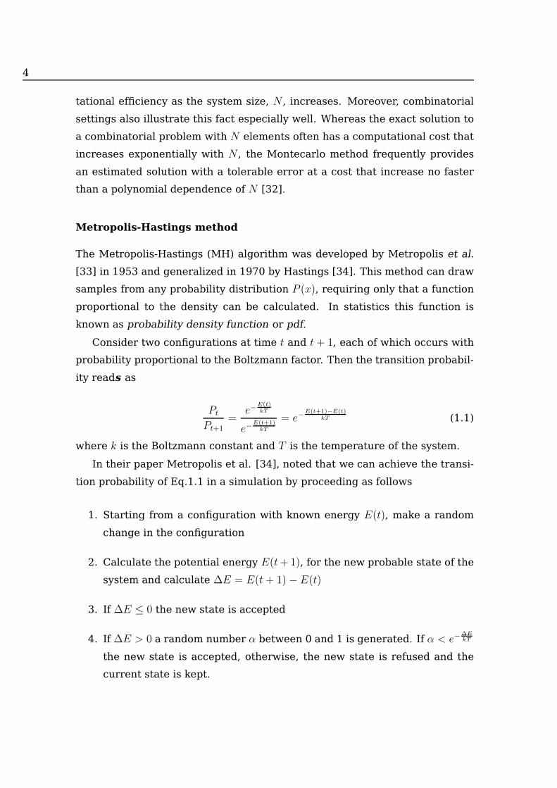
Metropolis-Hastings method
The Metropolis-Hastings (MH) algorithm was developed by Metropolis et al.
[33] in 1953 and generalized in 1970 by Hastings [34]. This method can draw
samples from any probability distribution P (x), requiring only that a function
proportional to the density can be calculated. In statistics this function is
known as probability density function or pdf.
Consider two configurations at time t and t + 1, each of which occurs with
probability proportional to the Boltzmann factor. Then the transition probabil-
ity reads as
Pt
Pt+1=
e−E(t)kT
e−E(t+1)
kT
= e−E(t+1)−E(t)
kT (1.1)
where k is the Boltzmann constant and T is the temperature of the system.
In their paper Metropolis et al. [34], noted that we can achieve the transi-
tion probability of Eq.1.1 in a simulation by proceeding as follows
1. Starting from a configuration with known energy E(t), make a random
change in the configuration
2. Calculate the potential energy E(t+1), for the new probable state of the
system and calculate ∆E = E(t+ 1)− E(t)
3. If ∆E ≤ 0 the new state is accepted
4. If ∆E > 0 a random number α between 0 and 1 is generated. If α < e−∆EkT
the new state is accepted, otherwise, the new state is refused and the
current state is kept.

Introduction 5
If we follow these rules, then we will sample on the phase space, all possi-
ble configurations with probability proportional to the Boltzmann factor. That
is consistent with the theory of equilibrium statistical mechanics. We can com-
pute average properties by summing them along the path we follow through
possible configurations. The ergodic hypothesis [35–38] states that an ensem-
ble average obtained by MC simulation is equivalent to an average time ob-
tained through a simulation of molecular dynamics in the limit of an adequate
sampling (MC) and sufficient time (MD). In physics and thermodynamics, the
ergodic hypothesis says that, over long periods of time, the time spent by
a particle in some region of the phase space of micro-states with the same
energy is proportional to the volume of this region, i.e., that all accessible
micro-states are equal-probable over a long period of time.
In the next chapter, we describe in details an example of MC called Direct
Simulation Monte Carlo (DSMC). The DSMC method was proposed by Graeme
Bird [39] and uses probabilistic (Monte Carlo) simulations to solve the Boltz-
mann equation. In our case, we examine the solution of the integro-differential
equation that describe the collision-induced fragmentation of a granular gas.
1.1.2 Molecular Dynamics
Molecular systems usually consist of a large number of interacting particles
whose typical size ranges from micrometers to nanometers. Very often, it
is impossible to describe such complex systems analytically, thus, numerical
methods are specially suited.
Molecular dynamic (MD) is a method commonly used to determine macro-
scopic thermodynamic properties of molecular systems. It was first intro-
duced by Alder and Wainwright in the 1950’s to study the interactions of hard
spheres [5, 6]. The next major advance was in 1964, when Rahman carried out
the first simulation using a realistic potential for liquid Argon [40]. In 1967,
Verlet calculated the full phase diagram of Argon, and computed correlation
functions testing several theories of the liquid state [41, 42].
MD describes deterministically the physical movements of atoms and molecules.
That’s why, it either requires the definition of a potential function, or a de-
6
scription of the terms by which the particles in the simulation will interact.
The force acting on a particle can be divided into two classes, short-range and
long-range forces. Short-range forces are the actions exerted by objects that
are near to the particle and that after a certain distance threshold becomes
zero, such as particles collisions. Long-range forces is said of those forces that
do not become equal to zero within any distance. Classic long-range forces are
gravity or external electrical fields.
The application of molecular dynamics algorithms to macroscopic systems
is called by the engineering community Discrete Elements Simulations (DEM).
This is generally distinguished by its inclusion of rotational degrees-of-freedom
as well as state-full contact and often complicated particle shape. Note that
the physics community does not make distinctions between molecular dynam-
ics (MD) and Discrete Elements Simulations (DEM).
Molecular dynamics simulation of granular system
Event-driven
In dilute systems, where the typical collision time is much shorter than the
mean time between successive collisions, particles are rarely in contact with
more than one particle. Hence, most of the time particles propagate along a
ballistic trajectory only interrupted by collisions with other particles. There-
fore, the pairwise collisions of particles can be considered as instantaneous
events, which may be treated separately [43].
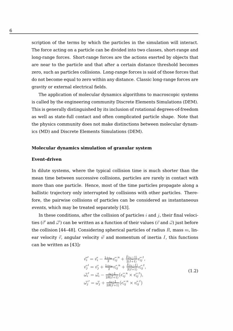
In these conditions, after the collision of particles i and j, their final veloci-
ties (~v′ and ~ω′) can be written as a function of their values (~v and ~ω) just before
the collision [44–48]. Considering spherical particles of radius R, mass m, lin-
ear velocity ~v, angular velocity ~w and momentum of inertia I, this functions
can be written as [43]:
~vi′ = ~vi − 1+ǫn
2~vij
n + I(ǫt−1)
2( ˜I+1)~vij
t,
~vj′ = ~vj +
1+ǫn2
~vijn + I(ǫt−1)
2( ˜I+1)~vij
t,
~ωi′ = ~ωi − ǫt−1
2R(I+1)( ~eij
n × ~vijt),
~ωj′ = ~ωj +
ǫt−12R(I+1)
( ~eijn × ~vij
t)
(1.2)

Introduction 7
where ~vij = ~vi− ~vj is the relative velocity, with components in normal ( ~vijn) and
tangential directions ( ~vijt). ~e represents a unit vector pointing along the line
of centers of mass from particle i to particle j and I = I/mR2 is the reduced
momentum of inertia. The normal restitution coefficient ǫn varies between 1
and 0, ǫn = 1 means no dissipation (elastic system) and ǫn = 0 means full
dissipation (perfectly inelastic system). The tangential restitution coefficient
ǫt = 1 goes from −1 (smooth particles) to +1 (rough particles), corresponding
to 0 the maximum coupling. The strength of the coupling between rotational
and translational motion is connected to 1 + ǫt [49–52].
Modeling event-driven MD, only one particle-particle interaction is con-
sidered each step of time. Moreover, the interaction takes an infinitesimal
time. On the time elapsed between two collisions, the particles move follow-
ing known ballistic trajectories. A general outline of the algorithm could be
1. Initialize positions ~ri, velocities ~vi and angular velocities ~ωi (if consid-
ered) for each particle i (i = 1, ..., N).
2. Calculate the time t∗ when the next collision occur. For equal-sized
spheres of radius R
t∗ ≡ min(| ~ri(tij)− ~rj(tij) | = 2R; i, j = 1, ..., N) (1.3)
3. Determine the position of all particles at t = t∗
~ri = ~ri + (t∗ − t)~vi + F exti (1.4)
where F exti are external long-range forces acting on particle i, as gravity.
4. Compute the new velocities accordingly to Equations 1.2.
5. Update the simulation time t = t∗.
6. Back to step 2 until the stop condition is satisfied.
The event-driven method is specially efficient for the study of dilute, non-
disperse, hard spheres materials [43, 52–55], but its application is not limited
to those systems [56–60]. In the presented algorithm, a constant restitution
coefficient is considered, some authors consider that this is not very realis-
tic [61, 62] and that the restitution coefficient should depend on the relative
velocity [46, 63–69].

8
Force-based molecular dynamics
In force-based molecular dynamics the forces that govern the motion of the
particles are determined from the (small) mutual deformation of the particles.
That’s why these methods are more appropriated for describing the micro-
mechanic properties of dense granular media and systems with complicated
particles shapes.
The general idea of molecular dynamics simulation is to numerically solve
the Newton’s equation of motion for all particles i (i = 1, ..., N)
N∑
j=1
~Fij + ~Fe = mi~ ir (1.5)
N∑
j=1
Lij = Iiθi (1.6)
wheremi is the mass of the particle, Ii is its moment of inertia and ~ri and θi are
the particle’s position and orientation respectively. ~Fe represents an external
field, ~Fij corresponds to the force exerted by particle j on particle i and Lij the
torque related with the force ~Fij, which points in the direction perpendicular
to the plane in which the particles displace. The total force and the total
torque acting on particle i are given as sums of the pair-wise interaction of
particle i with its contacting neighbors. Accordingly, the grains’ trajectories
will be determined by the nature of the collisional forces.
When two particles come in contact they deform inelastically. In force-
based molecular dynamics, rather than describing the actual grain deforma-
tions, the most common strategy consists in keeping the shape of the particles
and allow them to overlap. Hence, the interaction force and torque are deter-
mined in terms of the overlapping distance or area [43, 70–75].
The total force between the two grains, can be decomposed in normal FNij
and tangential F Tij components, to the interface defined by the contact points
of the two particles when they overlap
~Fij = FNij · ~n+ F T
ij · ~t (1.7)
Introduction 9
~n and ~t are the vectors in normal and tangential direction of the common
surface.
The normal component of the force contains an elastic contribution, pro-
portional to the pair overlapping distance or area, and a dissipative contribu-
tion FNij = FN
e + FNv . The tangential component of the interaction force is also
characterized by an elastic and a dissipative contribution F Tij = F T
e + F Tv , and
obeys the Coulomb constraint [76], F Tij 6 µ | FN
ij |, where µ stands for the
static friction coefficient
F Tij = −min(F T
ij , µFNij ) (1.8)
In general, for circular or spherical particles it is possible to derive analytic
expressions for FNij and F T
ij as a function of the overlapping distance. However,
for particles of irregular shape this is not feasible and it is computed numeri-
cally [43, 71–75, 77, 78].
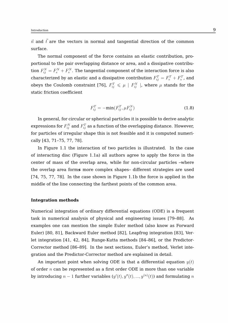
In Figure 1.1 the interaction of two particles is illustrated. In the case
of interacting disc (Figure 1.1a) all authors agree to apply the force in the
center of mass of the overlap area, while for non-circular particles –where
the overlap area forms more complex shapes– different strategies are used
[74, 75, 77, 78]. In the case shown in Figure 1.1b the force is applied in the
middle of the line connecting the farthest points of the common area.
Integration methods
Numerical integration of ordinary differential equations (ODE) is a frequent
task in numerical analysis of physical and engineering issues [79–88]. As
examples one can mention the simple Euler method (also know as Forward
Euler) [80, 81], Backward Euler method [82], Leapfrog integration [83], Ver-
let integration [41, 42, 84], Runge-Kutta methods [84–86], or the Predictor-
Corrector method [86–89]. In the next sections, Euler’s method, Verlet inte-
gration and the Predictor-Corrector method are explained in detail.
An important point when solving ODE is that a differential equation y(t)
of order n can be represented as a first order ODE in more than one variable
by introducing n− 1 further variables (y′(t), y′′(t), ..., y(n)(t)) and formulating n

10
a)
i
j
n t
b)
Ci
C j
FT
FN
FT
FN
Figure 1.1: Interaction of two particles. The normal force is parallel to the line that connect
the center of both particles and the tangential force is perpendicular to this imaginary line.
a) For interacting disc, the force is applied in the center of mass of the overlap area. b) When
non-regular particles are modeled different points are used to apply the force, in this case the
center of the line connecting the farthest vertex of the overlap area.
first-order equations in these new variables. For that reason, next epigraphs
focus on integration methods of first order differential equations.
Euler integration method
Euler’s method is the most basic first-order numerical method for solving
ODEs [80]. For using this approach two things are necessary, the differen-
tial equation and the value of the function at some point
dy
dt= f(t, y), y(t0) = y0 (1.9)
The method consist in approximate the solution of Equation 1.9 using the
linear approximation of y around the point P0(t0, y(t0)) (the first two terms of
the Taylor expansion [90])
yn+1 = yn + hf(tn, yn) (1.10)
where h = (tn+1 − tn) is known as the integration step. Equation 1.10 is cal-
culated iteratively until tn < tf . The algorithm in pseudocode is shown in
Algorithm 1.

Introduction 11
y(t0)← y0
n := 0
while tn < tf do
tn+1 := tn + h
yn+1 := yn + hf(tn, yn)
n := n+ 1
end while
Algorithm 1: Pseudocode of Euler’s method. It is the simplest and least accurate first-order
method for solving ODEs. The derivate yn+1 at each point tn+1 is calculated using the derivate
yn at the previous point tn.
The Euler’s method is unsymmetrical, it advances the solution through an
interval h, but uses derivative information only at the beginning of the interval.
That means that the step’s error is of the order of O(h2) [91]. A solution to
minimize the error is decreasing h, however, this action increase the number
of necessaries steps and therefore the computational cost.
This method is not recommended for most problems, mainly because it is
not accurate when compared to other methods running at equivalents step-
size and neither it is very stable [91].
Verlet integration method
Verlet integration was first used by Carl Störmer to compute the trajectories of
particles moving in a magnetic field (hence it is also called Störmer’s method)
[91] and was popularized in molecular dynamics by French physicist Loup
Verlet in 1967 [41, 42]. It is a numerical method used to integrate Newton’s
equations of motion (Equations 1.5 and 3.1) and frequently applied to calcu-
late trajectories of particles in molecular dynamics simulations and computer
graphics. The basic idea is to write two third-order Taylor expansions for the
positions r and orientations θ, one forward and one backward in time.
A related algorithm, and more commonly used in molecular dynamics sim-
ulations, is the Velocity Verlet algorithm, the basic implementation scheme of
this method is presented in Algorithm 2, for more details about the algorithm
see the section Appendix in [92].

12
a(t0)← 0
v(t0)← v0
t := 0
while t < tf do
v(t+ 12∆t) = v(t) + a(t)1
2∆t
x(t +∆t) = x(t) + v(t+ 12∆t)∆t
Derive a(t +∆t) from the forces equations using x(t +∆t)
v(t+∆t) = v(t+ 12∆t) + a(t +∆t)1
2∆t
t := t+∆t
end while
Algorithm 2: Pseudocode of Velocity Verlet method. It is a second-order method for solving
ODEs, developed for integrating the Newton’s equations of motion and with application in
physics and computational graphics. An intermediate integration is made at the mid-point
between tn and tn+∆t. The step size is called ∆t instead of h
The Verlet integrator offers greater stability, as well as time-reversibility
and preservation of the symplectic form on phase space, at no significant ad-
ditional cost over the Euler’s method. Nevertheless, the error is still of the
order of O(∆t2). The disadvantage of this method respect to Euler algorithm
consist in that, as it is calculated in three stages, it is more computationally
expensive, in both time and memory consuming.
Predictor-Corrector integration method
Predictor-corrector method consists of an implicit method of good accuracy
(corrector equation) and an explicit method (predictor equation) that provides
an initial approximation for the iterative process and the implicit method. Dif-
ferent implementations has been developed, those more often used in molec-
ular dynamics are due to C.W. Gear [87], and consists of three steps:
1. Predictor. From the positions and their derivatives up to order n in t are
obtained the same quantities at t+∆t by Taylor expansions. Among these
quantities are accelerations a. The predictor step for a fourth order Gear

Introduction 13
algorithm can be written in matrix form [44]
rp0(t+∆t)
rp1(t+∆t)
rp2(t+∆t)
rp3(t+∆t)
=
1 1 1 1
0 1 2 3
0 0 1 3
0 0 0 1
r0(t)
r1(t)
r2(t)
r3(t)
2. Forces. With the positions and the velocities predicted, forces are cal-
culated according to the contact model, and then the accelerations. The
difference between predicted accelerations and the ones calculated in
these step give the error of the method
∆r2(t+∆t) = rc2(t+∆t)− rp2(t +∆t)
3. Corrector. This error signal ǫ is used to correct positions and their
derivatives. The coefficients of proportionality are determined to max-
imize the stability of the method. In matrix form
rc0(t +∆t)
rc1(t +∆t)
rc2(t +∆t)
rc3(t +∆t)
=
rp0(t+∆t)
rp1(t+∆t)
rp2(t+∆t)
rp3(t+∆t)
c0
c1
c2
c3
∆r2(t+∆t)
In [87], C.W. Geard discusses the best choice for the corrector coeffi-
cients ci, which depends on how many derivatives of ri are used.
The main advantage of the predictor-corrector algorithm is its high accu-
racy. However, it is harder to implement and more time consuming (requires
additional calculations) and, numerically, is unstable against relatively big in-
tegration steps [93].
Boundary conditions
In general the behavior of granular systems are strongly influenced by the in-
teraction of the grains with the system boundaries, i.e., the interaction with
the container or the surface on which the system lays. As examples can be

14
Figure 1.2: A dilute granular system evolves in a circular container in the absence of external
forces. Initialized homogeneously (left), the particles accumulate close to the reflecting wall
after a long time (right). Taken from [43].
mentioned the convective motion of granular material in vibrating contain-
ers, the formation of density waves in pipes, the motion of granular materials
on conveyors, and the clogging of hoppers. In these cases, the interaction
with the container has to be examined carefully [43]. Hence, depending on
the applications the implemented boundaries should be different. The most
used types are reflecting boundaries, periodic boundary conditions and heated
walls. In the next section the first and second methods are explained. More-
over, some of their physical implications are discussed.
Reflecting Boundaries
There are two ways of applying reflecting boundary conditions: the first one,
when particles collide with the system walls its velocity component reverts
(conservatively or non-conservatively) perpendicular to the wall, whereas the
velocity component parallel to the wall remains invariant. The second method
is to build walls made of particles that follow the same interaction rules than
"internal particles" obey, varying –if necessary– the particle size. Such walls
are very simple to implement into the MD simulation due to no extra inter-
action rules are needed. The interaction of the particles with the wall are
computed in the same way that a particle-particle interaction.
Molecular dynamics simulations using reflecting boundaries shows strong
system size effect. For instance, after some time the particles clusterize near
Introduction 15
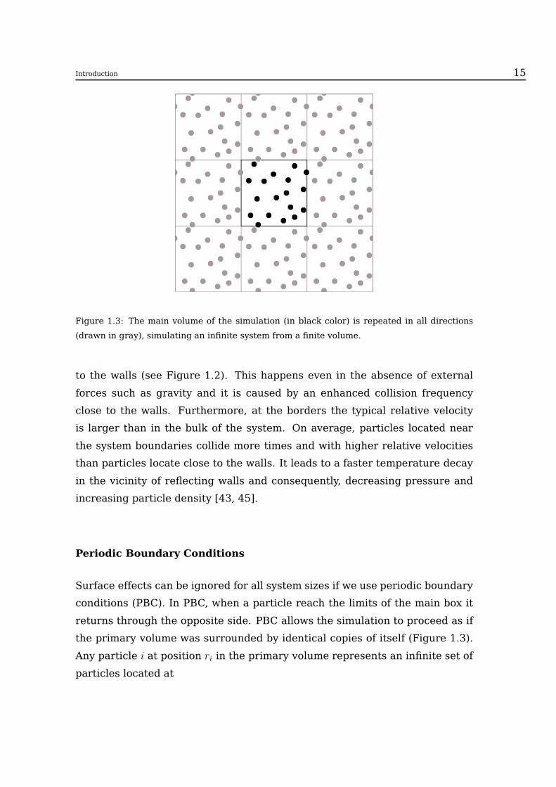
Figure 1.3: The main volume of the simulation (in black color) is repeated in all directions
(drawn in gray), simulating an infinite system from a finite volume.
to the walls (see Figure 1.2). This happens even in the absence of external
forces such as gravity and it is caused by an enhanced collision frequency
close to the walls. Furthermore, at the borders the typical relative velocity
is larger than in the bulk of the system. On average, particles located near
the system boundaries collide more times and with higher relative velocities
than particles locate close to the walls. It leads to a faster temperature decay
in the vicinity of reflecting walls and consequently, decreasing pressure and
increasing particle density [43, 45].
Periodic Boundary Conditions
Surface effects can be ignored for all system sizes if we use periodic boundary
conditions (PBC). In PBC, when a particle reach the limits of the main box it
returns through the opposite side. PBC allows the simulation to proceed as if
the primary volume was surrounded by identical copies of itself (Figure 1.3).
Any particle i at position ri in the primary volume represents an infinite set of
particles located at

16
~rk,l,mi = ~ri + k ~X + l~Y +m~Z (1.11)
where ~X, ~Y and ~Z are the edge vectors of the primary volume and k, l and m
are integer numbers taken values from −∞ to ∞. In practice the this set is
reduced to {−1, 0, 1}.Implementing periodic boundary conditions there are some important de-
tails to take into account:
1. Particles not only interact with those located in its volume, but also with
their periodic images.
2. A particle i can only interact with the closest image of particle j, i.e., two
particles i and j can not interact more than once in a single time step.
3. The distance between two particles i and j is the smallest distance be-
tween i and all images of j.
Moreover, it is important to remark that using PBC the studied system is
thought to be much larger than the simulated number of particles. In gen-
eral, the system size effects are smoothed and better controlled but not totally
diminished.
1.2 Scientific programming
General Overview
One of the major problems, currently faced by computational modeling re-
searchers, is the computational cost of the numerical algorithms, both in run-
time and memory usage. Moreover, the velocity of the new microprocessors is
not growing as fast as in the last years. An irrefutable evidence of this is that
the largest producers of microprocessors, Intel© Coorporation and AMD©
Inc., have stopped substantially increasing the clock speed of their processors
and have chosen to increase the number of cores.
With the introduction of multi-cores processors, computer programmers
have the option to develop their applications to run in parallel on their per-
sonal computers [94–96]. However, the use of multiple cores, specially when
Introduction 17
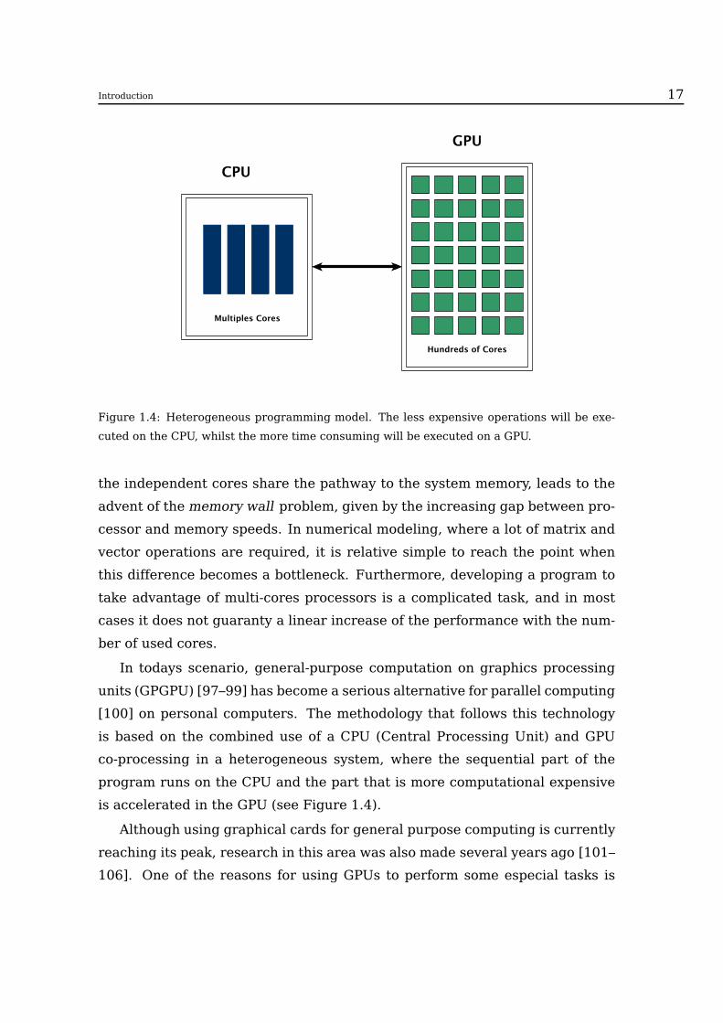
Figure 1.4: Heterogeneous programming model. The less expensive operations will be exe-
cuted on the CPU, whilst the more time consuming will be executed on a GPU.
the independent cores share the pathway to the system memory, leads to the
advent of thememory wall problem, given by the increasing gap between pro-
cessor and memory speeds. In numerical modeling, where a lot of matrix and
vector operations are required, it is relative simple to reach the point when
this difference becomes a bottleneck. Furthermore, developing a program to
take advantage of multi-cores processors is a complicated task, and in most
cases it does not guaranty a linear increase of the performance with the num-
ber of used cores.
In todays scenario, general-purpose computation on graphics processing
units (GPGPU) [97–99] has become a serious alternative for parallel computing
[100] on personal computers. The methodology that follows this technology
is based on the combined use of a CPU (Central Processing Unit) and GPU
co-processing in a heterogeneous system, where the sequential part of the
program runs on the CPU and the part that is more computational expensive
is accelerated in the GPU (see Figure 1.4).
Although using graphical cards for general purpose computing is currently
reaching its peak, research in this area was also made several years ago [101–
106]. One of the reasons for using GPUs to perform some especial tasks is
18
that CPUs are designed for high performance on sequential operations, while
GPUs are optimized for the high parallelism of vertex and fragment processing
[107].
Nowadays, to develop numerical applications on graphics cards there are
three choices NVIDIA© CUDA™, AMD© APP and OpenCL™
• CUDA is NVIDIA’s parallel computing architecture, giving to developers
the necessary tools to perform GPGPU on NVIDIA’s graphic cards [108].
• AMD APP technology is a set of advanced hardware and software tech-
nologies that enable AMD graphics processing cores, working in con-
cert with the system’s cores, to accelerate many applications beyond
just graphics using ATI graphic cards [109].
• OpenCL (Open Computing Language) is the first open, royalty-free stan-
dard for general-purpose parallel programming of heterogeneous sys-
tems. OpenCL provides a uniform programming environment for soft-
ware developers to write efficient, portable code for high-performance
compute servers [110].
Our research, in chapter 6 concerns NVIDIA CUDA, mainly because the
available GPU-hardware was NVIDIA’s graphic cards.
GPGPU with CUDA
In November 2006, NVIDIA© release the GeForce 8800 GTX, the first GPU
built with NVIDIA’s CUDA Architecture. This architecture included several
new components designed strictly for GPU computing, and aimed to allevi-
ate many of the limitations that prevented previous graphics processors from
being legitimately useful for general-purpose computation. Because NVIDIA
intended this new family of graphics processors to be used for GPGPU, the
processor’s ALUs (arithmetic logic unit) were built to comply with IEEE re-
quirements for single-precision floating-point arithmetic and were designed
to use an instruction set tailored for general computation rather than specifi-
cally for graphics [99].

Introduction 19
Figure 1.5: CPU and GPU Architecture. GPU devotes more transistors to data processing.
Taken from [111].
To reach the maximum number of developers, NVIDIA took industry-standard
C and added a relatively small number of keywords in order to harness some of
the special features of the CUDA Architecture. A few months after the launch
of its graphic card, NVIDIA made public a compiler for this language, CUDA
C, which became the first language specifically designed by a GPU company to
facilitate general-purpose computing on GPUs [99]. Nowadays there are third
party wrappers for many programming language, like: Python, Perl, Fortran,
Java, Ruby, MATLAB, and native support exists in Mathematica.
The reason behind the difference in performance of floating-point capabil-
ity between the CPU and the GPU is that the GPU is specialized for compute-
intensive, highly parallel computation. GPU are designed such that more tran-
sistors are devoted to data processing rather than data caching and flow con-
trol (see Figure 1.5). The GPU is especially well-suited to address problems
that can be expressed as data-parallel computations with high arithmetic in-
tensity –the ratio of arithmetic operations to memory operations. Because the
same program is executed for each data element, there is a lower requirement
for sophisticated flow control, and since it is executed on many data elements
and has high arithmetic intensity, the memory access latency can be hidden
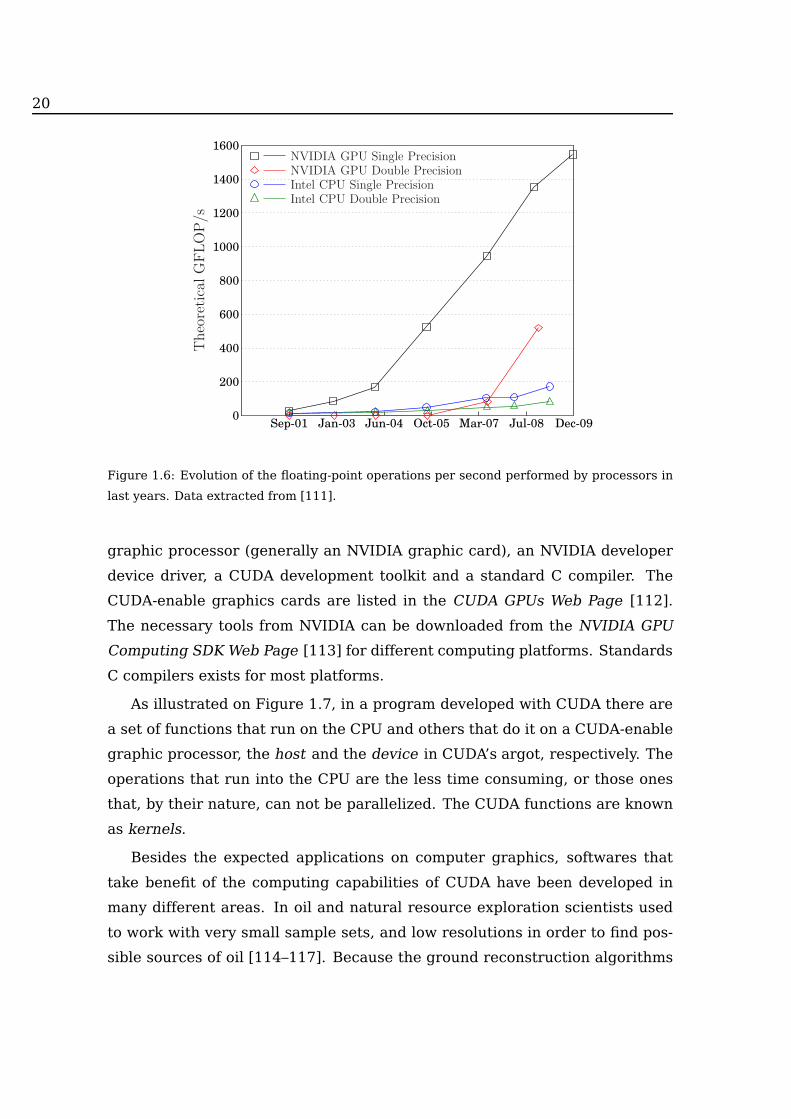
with calculations instead of big data caches [111]. The evolution of the num-
ber of floating-point operations per second (FLOP) that a processor can do is
shown in Figure 1.6.
To develop CUDA C applications it is indispensable to have a CUDA-enable
20
0
200
400
600
800
1000
1200
1400
1600
Sep-01 Jan-03 Jun-04 Oct-05 Mar-07 Jul-08 Dec-09
TheoreticalGFLOP/s
NVIDIA GPU Single PrecisionNVIDIA GPU Double PrecisionIntel CPU Single PrecisionIntel CPU Double Precision
Figure 1.6: Evolution of the floating-point operations per second performed by processors in
last years. Data extracted from [111].
graphic processor (generally an NVIDIA graphic card), an NVIDIA developer
device driver, a CUDA development toolkit and a standard C compiler. The
CUDA-enable graphics cards are listed in the CUDA GPUs Web Page [112].
The necessary tools from NVIDIA can be downloaded from the NVIDIA GPU
Computing SDK Web Page [113] for different computing platforms. Standards
C compilers exists for most platforms.
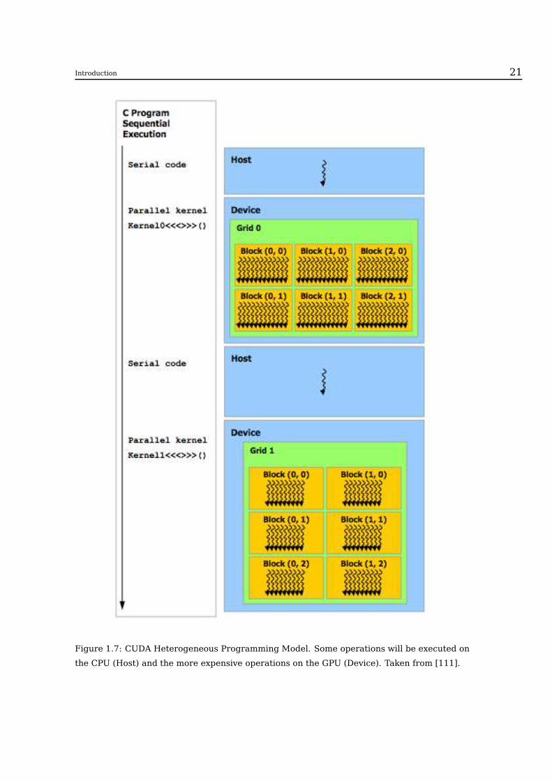
As illustrated on Figure 1.7, in a program developed with CUDA there are
a set of functions that run on the CPU and others that do it on a CUDA-enable
graphic processor, the host and the device in CUDA’s argot, respectively. The
operations that run into the CPU are the less time consuming, or those ones
that, by their nature, can not be parallelized. The CUDA functions are known
as kernels.
Besides the expected applications on computer graphics, softwares that
take benefit of the computing capabilities of CUDA have been developed in
many different areas. In oil and natural resource exploration scientists used
to work with very small sample sets, and low resolutions in order to find pos-
sible sources of oil [114–117]. Because the ground reconstruction algorithms
Introduction 21
Figure 1.7: CUDA Heterogeneous Programming Model. Some operations will be executed on
the CPU (Host) and the more expensive operations on the GPU (Device). Taken from [111].
22
are highly parallel, CUDA is perfectly suited to this type of challenge. For med-
ical imaging processing CUDA is a significant advancement [118–120]. Using
CUDA, MRI machines can now compute images faster than ever possible be-
fore, and for a lower price. Before CUDA, it used to take an entire day to make
a diagnosis of breast cancer and now this can take only 30 minutes.
In chapter 6 we describe in detail the implementation of a hybrid CPU-
GPU molecular dynamics algorithm of dissipative spheres including rotation.
Starting from the crude CUDA-particles example we have developed a very
accurate algorithm for examining a realistic granular system.
Chapter 2
Collision induced fragmentation:
a simple numerical algorithm
Fragmentation processes are of significant scientific interest and have enor-
mous technological impact. These phenomena usually arise in many natural
and technological processes, such as granulate processing [121], shattering of
solid and shell-like objects [122–124], meteorite [125], mineral grinding [126],
liquid droplets [127] and atomic nuclei [128]. In some cases fragmentation can
be regarded as linear. That is the case when the process dynamics is only sen-
sitive particle properties (such as size) and it does not depend significantly
on particle interaction [129]. Contrary, when the interaction between grains
plays a significant role the evolution of the granular system is intrinsically
non-linear.
Most of the theoretical studies on fragmentation have been carried out
within the framework of Smoluchowski-like equations[129–134], where parti-
cle fragmentation is determined by impacts of pairs of particles. Here, the
role of particle velocity at impact is neglected, and the evolution of the distri-
bution of particle sizes have been described. These studies have led to explicit
results and have addressed the emergence and properties of dynamic scaling
regimes [129–137]. Although less explored, the effect of particle velocity at
collision and its relevance in fragmentation has also been addressed recently
[137–139].
McGrady and Ziff realized that under special circumstances a fragmenting
23

24
system can give rise to a singularity the so-called shattering transition [130].
This refers to a finite time, tc, at which a finite fraction of the system mass
is carried by an infinite number of particles of infinitesimal size, which can
be regarded as dust [130, 132–134]. This transition shares close analogies
with the reverse process of gelation in aggregation kinetics, which has also
been analyzed in the context of the Smoluchowski equation where aggrega-
tion arises as a result of two particle interactions [140–142]. The particular
details of the collision-induced fragmentation process may lead to different
types of shattering transitions, which may resemble first or second-order non-
equilibrium phase transitions [133, 134]. Specifically, at the transition either
the entire mass of the system is instantly transformed into dust or the dust
mass gradually increases once the shattering transition occurred.
Because of its complexity, explicit solutions of generic non-linear fragmen-
tation equations are generally not accessible. Hence, in generic cases a de-
tailed study of the dynamics of fragmenting systems requires the use of nu-
merical tools. To this end, we have adapted the Direct Simulation Monte Carlo
(DSMC) technique, which has been widely used in the context of rarefied gases
[143] and granular gases [144, 145], to the study of non-linear fragmenting
systems.
2.1 Mean Field Theory
Collision-induced fragmentation can be described at the mean field level by
the Smoluchowski fragmentation equation of the massdensity c(x, t) as
∂c(x, t)/∂t = −c(x, t)∫∞0dyK(x, y)c(y, t) +
∫∞xdy
∫∞0
dz b(x|y) K(y, z)c(y, t)c(z, t)
(2.1)
which assumes binary collisions and the kernel K(x, y) describes the interac-
tion rate of pairs of particles [x; y]. Equation (2.1) is composed of a loss (first)
and a gain (second) term [131]. In the gain term, b(x|y) represents a con-
ditional probability which describes the distribution of outgoing fragments of
mass x, given that a particle of mass y breaks [130, 131]. Here, one may distin-
guish between deterministic kinetics [131, 133], where a particle breaks into
two equal fragments, hence b(x|y) = 2δ(x− y/2), and stochastic fragmentation
Collision induced fragmentation: a simple numerical algorithm 25
processes, where a fragment of random mass x breaks off from a particle of
mass y. As mass is conserved in a single breakup event, the outgoing fragment
distribution has to obey the homogeneity requirement, of b(x|y) = y−1b(xy). For
simplicity, the standard form b(s) = (β + 2)sβ is adopted and it obeys∫ y
0dxxb(x|y) = y, N =
∫ y
0dxb(x|y) = β+2
β+1(2.2)
where N is the mean number of outgoing fragments, which satisfies N ≥ 2,
and implies −1 < β ≤ 0. Binary breakup corresponds to β = 0.
The size dependence of the collision kernels depends on the physical pro-
cesses underlaying particle interactions. A variety of collision kernels,K(x, y),
has been proposed in applications of the non-linear Smoluchowski equation
[140, 141, 146]. Because of their physical motivation and mathematical sim-
plicity, most kernels have a sum-product form, such as
K(x, y) = 1, xp + yp, (xy)p, xpyq + xqyp (2.3)
In Equation (2.1), the kernel K(x, y) may also contain the probability that
breakage indeed occurs, expressed as p(x, y). Although in general, it will de-
pends on particles’ properties, if we can assume it as a constant we can al-
ready identify three classes of fragmentation kinetics depending on whether
particle x or y breaks: (i) symmetric breakage, where a randomly chosen par-
ticle of the interacting pair (x, y) breaks [131, 133], and where p(x, y) = 1;
(ii)L-breakage, where the larger particle breaks, hence p(x, y) = θ(x− y); and
(iii) S-breakage, where the smaller particle breaks and p(x, y) = θ(y − x); θ(x)
stands for the unit step function. The general expression, Eq.( 2.1) reduces
for L-breakage and S-breakage to
∂c(x, t)
∂t= −c(x)
∫∞0dyK(x, y)θ(x− y)c(y) +
∫∞xdy
∫∞0
dzb(x|y)K(y, z)θ(y − z)c(y)c(z)
∂c(x, t)
∂t= −c(x)
∫∞0dyK(x, y)θ(y − x)c(y) +
∫∞xdy
∫∞0
dzb(x|y)K(y, z)θ(z − y)c(y)c(z)(2.4)
respectively.
2.2 Direct Simulation Monte Carlo Algorithm
Due to the non-linear character of the Smoluchowski fragmentation equation,
it is useful to develop a numerical scheme which can explore efficiently the
26
main features of fragmentation kinetics. To this end, we have developed a
numerical approach which follows the basic idea of Direct Simulation Monte
Carlo (DSMC) technique, introduced by Bird to directly simulate the Boltz-
mann equation [143], and which has been extended to study other systems,
such as granular gases [144]. The general idea underlying the approach is
easily generalized to other kinetic equations.
Instead of solving Equation (2.1) numerically, we follow its temporal evolu-
tion through a stochastic sampling of the fragmentation process. We represent
the fragmentation system by N particles with variable masses. These parti-
cles, however, do not correspond to real particles, they rather represent the
continuum distribution which evolves according to the fragmentation equa-
tion. We follow the basic scheme in DSMC and fix a time step ∆t0, smaller
than the characteristic relaxation time of the kinetic equation. We then take
a pair of particles at random, i and j with masses xi and xj respectively, and
make them fragment with a probability
Pcoll(i, j) =wij
∑Nn=1
∑N−1m=1 wnm
(2.5)
where we define the fragmentation frequency
wij ≡ K(xi, yj) (2.6)
Following DSMC, we avoid the expensive calculation of the denominator
by estimating the largest fragmentation frequency, wmax, and accept fragmen-
tation events with a probability Pcoll(i, j) = wij/wmax. One can also compute
the number of pairs that must be sampled during ∆t0, since the number of
colliding pairs is fixed by the fragmentation frequency
Mcoll = N2〈w〉∆t0 (2.7)
where 〈w〉 stands for the averaged fragmentation frequency during the corre-
sponding time interval. In order to maintain the proper fragmentation prob-
ability, we must then sample Msample = N2wmax∆to pairs. For the particular
choice ∆t0 = 1/N2wmax, it is enough to increment the time by an amount ∆t0
after each attempt to fragment a pair of particles.

Collision induced fragmentation: a simple numerical algorithm 27
Instead of using a fixed time increment, it is possible to use the previous
discussion considering that to observe a collision one needs to try to fragment
Msample = wmax/〈w〉 pairs. Hence, wmax/〈w〉 trials need to be carried out before
a pair is fragmented, which corresponds to a fragmentation probability of
P (w) =w
N(N−1)2〉/wmax
(2.8)
Only when a pair fragments is time is incremented by the amount
∆t =1
N2wmax(2.9)
to ensure consistency with the previous scheme for a prescribed, constant
time step. Making use of the fragmentation probability associated with this
scheme, the mean time step can be derived from the expression for the general
moments of the fragmentation distribution
〈∆tn〉 =∑
i
∑
j
wij
N(N−1)2〈w〉
(
1
N2wij
)n
=1
〈w〉N2〈 1
(N2w)n−1〉 (2.10)
where 〈w〉 =∑
i
∑
j wij/(N(N − 1)/2). As anticipated, from the previous ex-
pression for the moments of the distribution we can derive in particular the
mean time step, 〈dt〉 = 1/(N2〈w〉), consistent with Equation (2.9).
Once the fragmentation event is accepted, we need to decide whether par-
ticle i or j will subsequently break. In this work, we study symmetric frag-
mentation, where a randomly chosen particle breaks [131, 133] and asymmet-
ric fragmentation where either the larger L-breakage or the smaller particle
S-breakage breaks [133]. We also distinguish between deterministic fragmen-
tation [131, 133], where the chosen particle breaks into two equal fragments,
and stochastic fragmentation, where the chosen particle breaks randomly into
two off-springs. By following this procedure, it is possible to keep track of the
kinetic evolution of the system, as well as gather statistics on the distribution
of sizes.
In the next sections, we validate the proposed algorithm by comparing the
results of kinetic evolution and statistics of sizes with previous analytical find-
ings for symmetric and asymmetric kernels. In addition, the method allow us
to examine the L-breakage and S-breakage models for generic kernelsK(x, y),
for which no exact scaling solutions are known.
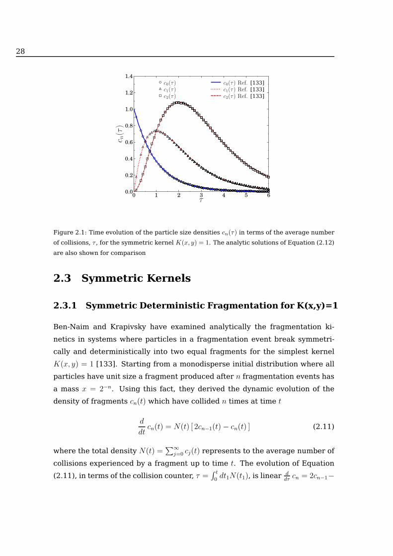
28
0.0
0.2
0.4
0.6
0.8
1.0
1.2
1.4
0 1 2 3 4 5 6
c n(τ
)
τ
c0(τ)c1(τ)c2(τ)
c0(τ) Ref.c1(τ) Ref.c2(τ) Ref. [133]
[133][133]
Figure 2.1: Time evolution of the particle size densities cn(τ) in terms of the average number
of collisions, τ , for the symmetric kernel K(x, y) = 1. The analytic solutions of Equation (2.12)
are also shown for comparison
2.3 Symmetric Kernels
2.3.1 Symmetric Deterministic Fragmentation for K(x,y)=1
Ben-Naim and Krapivsky have examined analytically the fragmentation ki-
netics in systems where particles in a fragmentation event break symmetri-
cally and deterministically into two equal fragments for the simplest kernel
K(x, y) = 1 [133]. Starting from a monodisperse initial distribution where all
particles have unit size a fragment produced after n fragmentation events has
a mass x = 2−n. Using this fact, they derived the dynamic evolution of the
density of fragments cn(t) which have collided n times at time t
d
dtcn(t) = N(t) [ 2cn−1(t)− cn(t) ] (2.11)
where the total density N(t) =∑∞
j=0 cj(t) represents to the average number of
collisions experienced by a fragment up to time t. The evolution of Equation
(2.11), in terms of the collision counter, τ =∫ t
0dt1N(t1), is linear
ddτ
cn = 2cn−1−
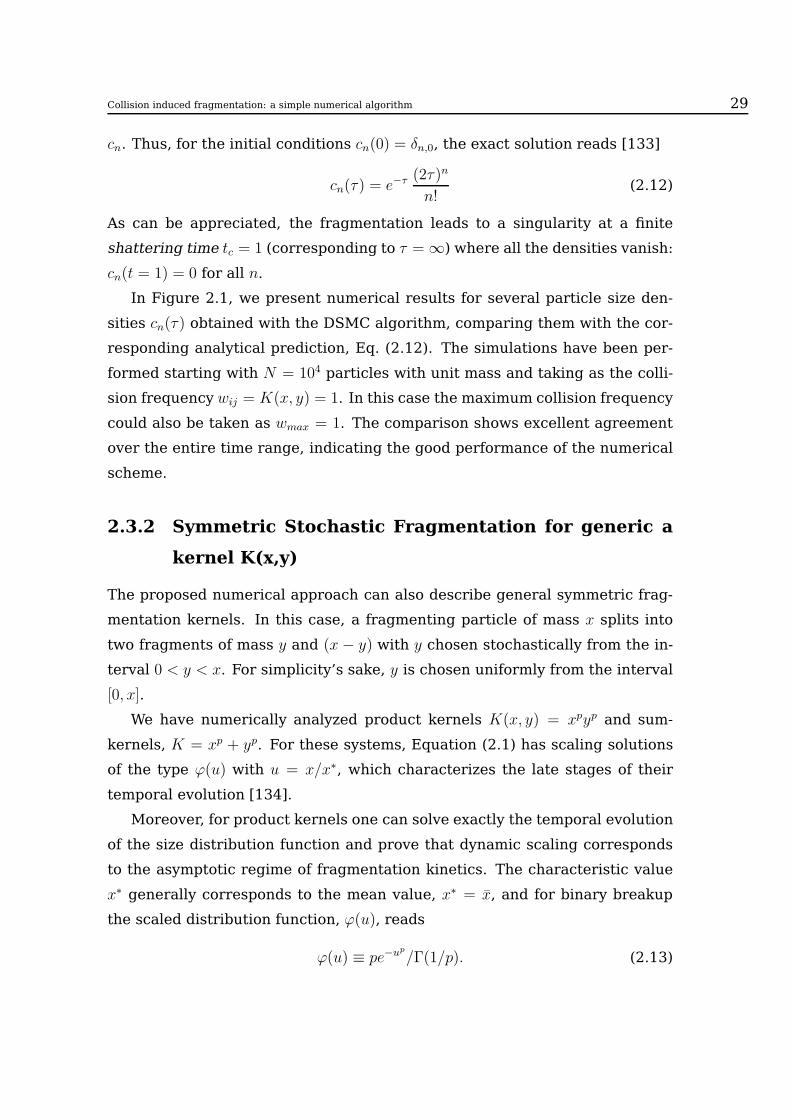
Collision induced fragmentation: a simple numerical algorithm 29
cn. Thus, for the initial conditions cn(0) = δn,0, the exact solution reads [133]
cn(τ) = e−τ (2τ)n
n!(2.12)
As can be appreciated, the fragmentation leads to a singularity at a finite
shattering time tc = 1 (corresponding to τ =∞) where all the densities vanish:
cn(t = 1) = 0 for all n.
In Figure 2.1, we present numerical results for several particle size den-
sities cn(τ) obtained with the DSMC algorithm, comparing them with the cor-
responding analytical prediction, Eq. (2.12). The simulations have been per-
formed starting with N = 104 particles with unit mass and taking as the colli-
sion frequency wij = K(x, y) = 1. In this case the maximum collision frequency
could also be taken as wmax = 1. The comparison shows excellent agreement
over the entire time range, indicating the good performance of the numerical
scheme.
2.3.2 Symmetric Stochastic Fragmentation for generic a
kernel K(x,y)
The proposed numerical approach can also describe general symmetric frag-
mentation kernels. In this case, a fragmenting particle of mass x splits into
two fragments of mass y and (x − y) with y chosen stochastically from the in-
terval 0 < y < x. For simplicity’s sake, y is chosen uniformly from the interval
[0, x].
We have numerically analyzed product kernels K(x, y) = xpyp and sum-
kernels, K = xp + yp. For these systems, Equation (2.1) has scaling solutions
of the type ϕ(u) with u = x/x∗, which characterizes the late stages of their
temporal evolution [134].
Moreover, for product kernels one can solve exactly the temporal evolution
of the size distribution function and prove that dynamic scaling corresponds
to the asymptotic regime of fragmentation kinetics. The characteristic value
x∗ generally corresponds to the mean value, x∗ = x, and for binary breakup
the scaled distribution function, ϕ(u), reads
ϕ(u) ≡ pe−up
/Γ(1/p). (2.13)
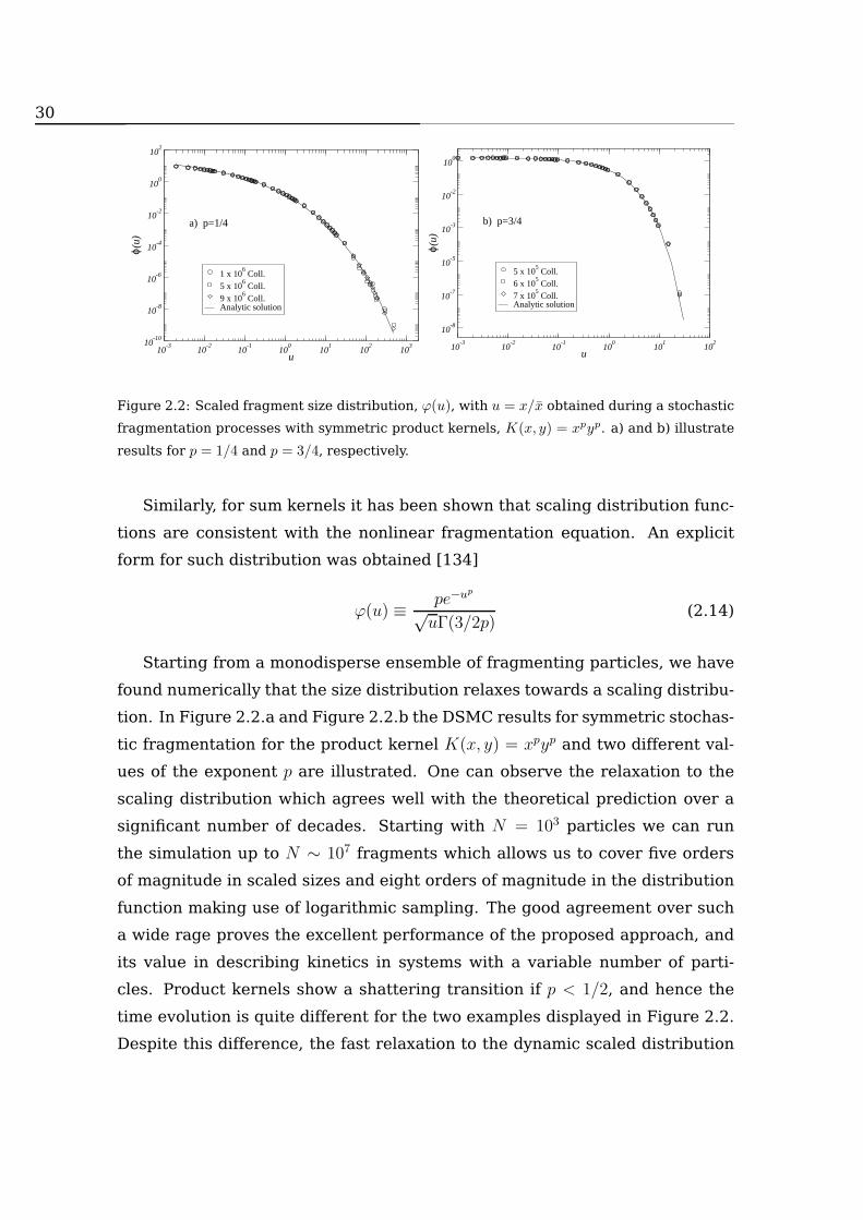
30
10-3
10-2
10-1
100
101
102
103
u
10-10
10-8
10-6
10-4
10-2
100
102
ϕ(u)
1 x 10⁶ Coll.
5 x 10⁶ Coll.
9 x 10⁶ Coll.
Analytic solution
a) p=1/4
10-3
10-2
10-1
100
101
102
u
10-8
10-7
10-5
10-3
10-2
100
ϕ(u)
5 x 10⁵ Coll.
6 x 10⁵ Coll.
7 x 10⁵ Coll.
Analytic solution
b) p=3/4
Figure 2.2: Scaled fragment size distribution, ϕ(u), with u = x/x obtained during a stochastic
fragmentation processes with symmetric product kernels, K(x, y) = xpyp. a) and b) illustrate
results for p = 1/4 and p = 3/4, respectively.
Similarly, for sum kernels it has been shown that scaling distribution func-
tions are consistent with the nonlinear fragmentation equation. An explicit
form for such distribution was obtained [134]
ϕ(u) ≡ pe−up
√uΓ(3/2p)
(2.14)
Starting from a monodisperse ensemble of fragmenting particles, we have
found numerically that the size distribution relaxes towards a scaling distribu-
tion. In Figure 2.2.a and Figure 2.2.b the DSMC results for symmetric stochas-
tic fragmentation for the product kernel K(x, y) = xpyp and two different val-
ues of the exponent p are illustrated. One can observe the relaxation to the
scaling distribution which agrees well with the theoretical prediction over a
significant number of decades. Starting with N = 103 particles we can run
the simulation up to N ∼ 107 fragments which allows us to cover five orders
of magnitude in scaled sizes and eight orders of magnitude in the distribution
function making use of logarithmic sampling. The good agreement over such
a wide rage proves the excellent performance of the proposed approach, and
its value in describing kinetics in systems with a variable number of parti-
cles. Product kernels show a shattering transition if p < 1/2, and hence the
time evolution is quite different for the two examples displayed in Figure 2.2.
Despite this difference, the fast relaxation to the dynamic scaled distribution
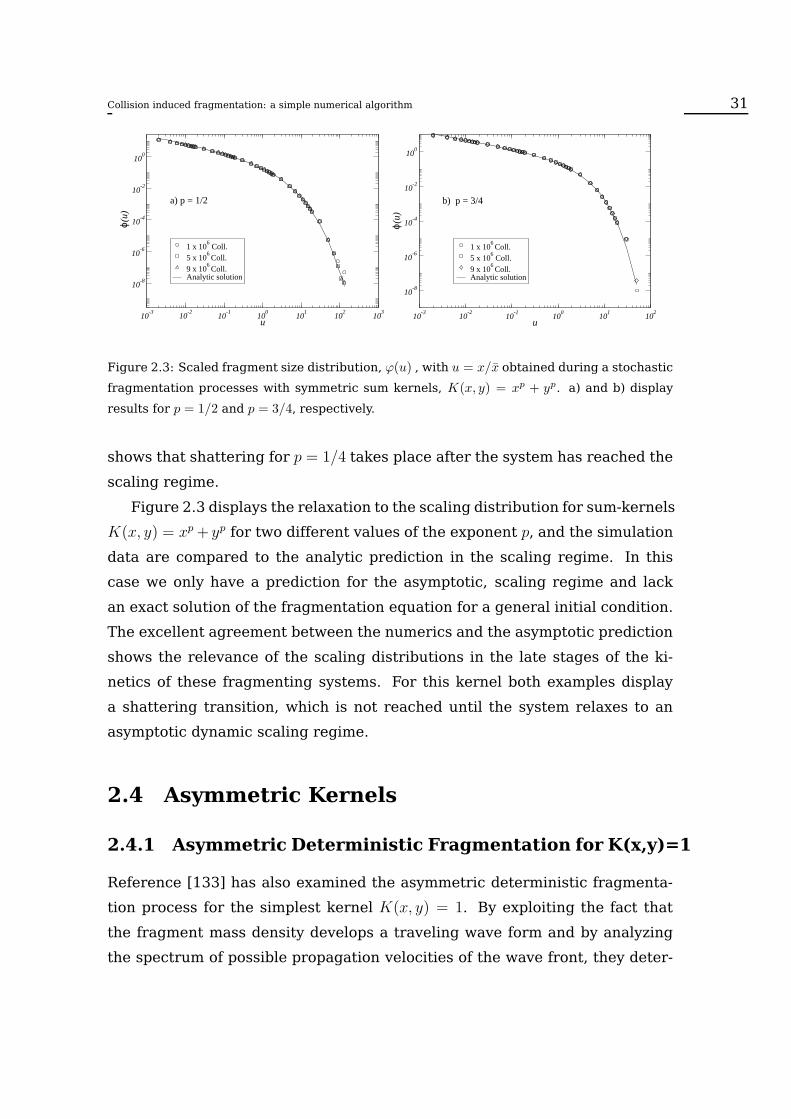
Collision induced fragmentation: a simple numerical algorithm 31
10-3
10-2
10-1
100
101
102
103
u
10-8
10-6
10-4
10-2
100
ϕ(u
)
1 x 10⁶ Coll.
5 x 10⁶
Coll.9 x 10
6 Coll.
Analytic solution
a) p = 1/2
10-3
10-2
10-1
100
101
102
u
10-8
10-6
10-4
10-2
100
ϕ(u)
1 x 10⁶
Coll.5 x 10
6 Coll.
9 x 10⁶
Coll.Analytic solution
b) p = 3/4
Figure 2.3: Scaled fragment size distribution, ϕ(u) , with u = x/x obtained during a stochastic
fragmentation processes with symmetric sum kernels, K(x, y) = xp + yp. a) and b) display
results for p = 1/2 and p = 3/4, respectively.
shows that shattering for p = 1/4 takes place after the system has reached the
scaling regime.
Figure 2.3 displays the relaxation to the scaling distribution for sum-kernels
K(x, y) = xp + yp for two different values of the exponent p, and the simulation
data are compared to the analytic prediction in the scaling regime. In this
case we only have a prediction for the asymptotic, scaling regime and lack
an exact solution of the fragmentation equation for a general initial condition.
The excellent agreement between the numerics and the asymptotic prediction
shows the relevance of the scaling distributions in the late stages of the ki-
netics of these fragmenting systems. For this kernel both examples display
a shattering transition, which is not reached until the system relaxes to an
asymptotic dynamic scaling regime.
2.4 Asymmetric Kernels
2.4.1 Asymmetric Deterministic Fragmentation for K(x,y)=1
Reference [133] has also examined the asymmetric deterministic fragmenta-
tion process for the simplest kernel K(x, y) = 1. By exploiting the fact that
the fragment mass density develops a traveling wave form and by analyzing
the spectrum of possible propagation velocities of the wave front, they deter-

32
0.2
0.4
0.6
0.8
1.0
-6 -4 -2 0 2 4
0.2
0.4
0.6
0.8
1.0
-5 0 5 10 15 20 25 30
Fn(τ
)
n− vτ
n=2
n=4
n=6
n=8
n=10
a) Big
1−
Fn(τ
)
n− vτ
n=18
n=24
n=26
n=28
n=30
b) Small
Figure 2.4: Evolution of the normalized cumulative size density Fn(n − vτ) for deterministic
fragmentation, using the asymmetric kernels a) K(x, y) = θ(x − y) and b) K(x, y) = θ(y − x).
The opposed asymptotic behavior of Fn(n − vτ) in the two cases is related to the different
properties of the densities linked to the details of the fragmentation process.
mined that the extremal front velocity characterizes the asymptotic behavior
of the mass distribution.
Larger particle splits. K(x, y) = θ(x− y)
In the case the larger particle fragments deterministically, after n fragmenta-
tion events a particle with an initial mass of x = 1 will have a mass of x = 2−n.
Thus, the density cn(t) of particles which have experienced n fragmentation
events at time t reads
d
dtcn = 4cn−1An − 2cnAn+1 + 2c2n−1 − c2n (2.15)
where An is the cumulative density of fragments of mass 2−n and smaller, and
An(t) =∑∞
j=n cj(t). As a result, starting from a monodisperse system, the
density c0(t) of unit mass particles gives
c0(t) =3(1− t)2
2 + (1− t)3. (2.16)
Equation (2.15) notably simplifies in terms of the normalized cumulative den-
sities Fn(τ) = N−1An(t), which obey a non-linear evolution equation
d
dτFn = 2F 2
n−1 − F 2n − Fn (2.17)
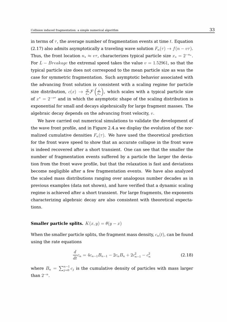
Collision induced fragmentation: a simple numerical algorithm 33
in terms of τ , the average number of fragmentation events at time t. Equation
(2.17) also admits asymptotically a traveling wave solution Fn(τ)→ f(n− vτ).
Thus, the front location n∗ ≈ vτ , characterizes typical particle size x∗ = 2−n∗.
For L − Breakage the extremal speed takes the value v = 1.52961, so that the
typical particle size does not correspond to the mean particle size as was the
case for symmetric fragmentation. Such asymptotic behavior associated with
the advancing front solution is consistent with a scaling regime for particle
size distribution, c(x) → Nx∗
F(
xx∗
)
, which scales with a typical particle size
of x∗ = 2−vτ and in which the asymptotic shape of the scaling distribution is
exponential for small and decays algebraically for large fragment masses. The
algebraic decay depends on the advancing front velocity, v.
We have carried out numerical simulations to validate the development of
the wave front profile, and in Figure 2.4.a we display the evolution of the nor-
malized cumulative densities Fn(τ). We have used the theoretical prediction
for the front wave speed to show that an accurate collapse in the front wave
is indeed recovered after a short transient. One can see that the smaller the
number of fragmentation events suffered by a particle the larger the devia-
tion from the front wave profile, but that the relaxation is fast and deviations
become negligible after a few fragmentation events. We have also analyzed
the scaled mass distributions ranging over analogous number decades as in
previous examples (data not shown), and have verified that a dynamic scaling
regime is achieved after a short transient. For large fragments, the exponents
characterizing algebraic decay are also consistent with theoretical expecta-
tions.
Smaller particle splits. K(x, y) = θ(y − x)
When the smaller particle splits, the fragment mass density, cn(t), can be found
using the rate equations
d
dtcn = 4cn−1Bn−1 − 2cnBn + 2c2n−1 − c2n (2.18)
where Bn =∑n−1
j=0 cj is the cumulative density of particles with mass larger
than 2−n.
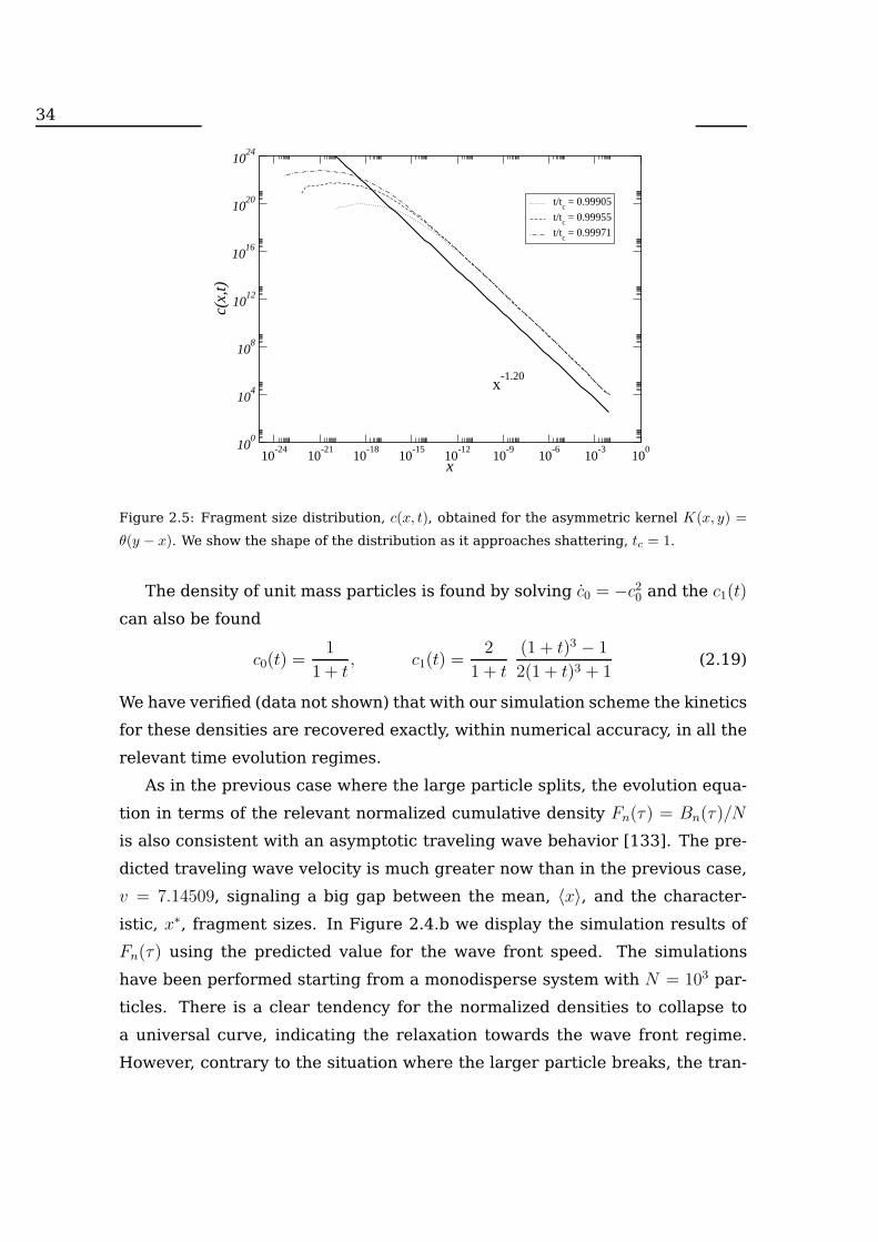
34
10-24
10-21
10-18
10-15
10-12
10-9
10-6
10-3
100
x
100
104
108
1012
1016
1020
1024
c(x,
t)t/t
c = 0.99905
t/tc = 0.99955
t/tc = 0.99971
x-1.20
Figure 2.5: Fragment size distribution, c(x, t), obtained for the asymmetric kernel K(x, y) =
θ(y − x). We show the shape of the distribution as it approaches shattering, tc = 1.
The density of unit mass particles is found by solving c0 = −c20 and the c1(t)
can also be found
c0(t) =1
1 + t, c1(t) =
2
1 + t
(1 + t)3 − 1
2(1 + t)3 + 1(2.19)
We have verified (data not shown) that with our simulation scheme the kinetics
for these densities are recovered exactly, within numerical accuracy, in all the
relevant time evolution regimes.
As in the previous case where the large particle splits, the evolution equa-
tion in terms of the relevant normalized cumulative density Fn(τ) = Bn(τ)/N
is also consistent with an asymptotic traveling wave behavior [133]. The pre-
dicted traveling wave velocity is much greater now than in the previous case,
v = 7.14509, signaling a big gap between the mean, 〈x〉, and the character-
istic, x∗, fragment sizes. In Figure 2.4.b we display the simulation results of
Fn(τ) using the predicted value for the wave front speed. The simulations
have been performed starting from a monodisperse system with N = 103 par-
ticles. There is a clear tendency for the normalized densities to collapse to
a universal curve, indicating the relaxation towards the wave front regime.
However, contrary to the situation where the larger particle breaks, the tran-

Collision induced fragmentation: a simple numerical algorithm 35
0.2
0.4
0.6
0.8
1.0
-2 -1 0 1 2 3 4 5 6 7
0.2
0.4
0.6
0.8
1.0
-5 0 5 10 15 20 25 30 35 40
Fn(τ
)
n− vτ
n=4
n=6
n=8
n=10
a) Big
1−
Fn(τ
)n− vτ
n=18
n=24
n=26
n=34
n=44
b) Small
Figure 2.6: Evolution of the normalized cumulative size density, Fn(n − vτ), for stochastic
fragmentation, using the asymmetric kernels a) K(x, y) = θ(x − y) and b) K(x, y) = θ(y − x).
sient is now much longer, as can be appreciated from the deviations from the
scaling solution. One can see that the relaxation to the asymptotic wave front
becomes heterogeneous. This slower relaxation to the traveling wave pat-
tern also implies that mass distribution will approach the scaling asymptotic
limit more slowly, as displayed in Figure 2.5. This model shows a shattering
transition at tc =1No; the figure illustrates how the predicted algebraic decay,
c(x, t) ∼ x−α with α ≃ 1.20191 is reached for large masses, while deviations for
small sizes still remain very close to shattering. In order to analyze carefully
the slow convergence to scaling, and to sample the widest possible range, we
have run simulations to reach up to N = 108 fragments. In performing these
simulations the scaled distribution functions span five orders of magnitude in
rescaled sizes (data not shown).
2.4.2 Asymmetric Stochastic Fragmentation
The asymmetric fragmentation model with stochastic breaking has also been
analyzed analytically for the simplest uniform fragmentation kernel, i.e. K(x, y) =
θ(x − y) for L-Breakage and K(x, y) = θ(y − x) for S-Breakage. Using the
same theoretical approach as explained in the previous sections, it has been

36
0.2
0.4
0.6
0.8
1.0
-2 0 2 4 6 8 10 12
.............
......
.
0.2
0.4
0.6
0.8
1.0
-2 0 2 4 6 8 10
....................
.
1−
Fn(τ
)
n− vτ
n=2
n=4
n=6
n=8
n=10
n=12
a) 1
2
1−
Fn(τ
)n− vτ
n=2
n=4
n=6
n=8
n=10
n=12
b) 3
4p =p =
Figure 2.7: Evolution of the normalized cumulative size density, Fn(n − vτ), for stochastic
fragmentation, using the asymmetric product kernel K(x, y) = θ(x − y)xpyp. Results shown
for a) p = 1/2 and b) p = 3/4, respectively
shown that both for large and small particle breakage the evolution of the nor-
malized cumulative densities relaxes asymptotically to a front wave solution,
Fn(τ) → f(n − vτ). For large particle fragmentation, v = 1, and hence the
characteristic and mean size coincide, while for small particle fragmentation
v = 9, which is larger than the deterministic fragmentation counterpart.
In Figure (2.6) we display Fn(τ) in both cases to show the convergence
to the wave front solution using the theoretical predictions for v. As it was
the case for asymmetric deterministic fragmentation, the convergence to the
scaling asymptotic regime is slower for small particle breakage, while for large
breakage it seems faster than in the deterministic case. One may speculate
that the deviation between the mean and the typical masses induces additional
kinetic heterogeneity which slows the relaxation to the asymptotic regime.
We have also verified that the scaled mass distribution is also reached (data
not shown) and that the distributions observed are consistent with theoretical
predictions. Again, in accordance with the results obtained for Fn(τ), the
convergence to the scaling distribution c(x, 1) ∼ x−α with α = 10/9 for x >> x∗
for small breakage is slower and more heterogeneous than for L-Breakage
(data not shown).
Collision induced fragmentation: a simple numerical algorithm 37
10-3
10-2
10-1
100
101
102
103
u
10-7
10-5
10-2
100
ϕ(u)
9 x 10⁵
Coll.1 x 10
6 Coll.
2 x 10⁶
Coll.u
-2
10-3
10-2
10-1
100
101
102
103
u
10-7
10-5
10-2
100
ϕ(u)
9 x 10⁵ Coll.
1 x 10⁶ Coll.
2 x 10⁶ Coll.
u-5/2
Figure 2.8: Scaled fragment size distribution, ϕ(u), with u = x/x∗ for a stochastic fragmenta-
tion with an asymmetric product kernel K(x, y) = θ(x − y)xpyp. The density distributions for
a) p = 1/2 and b) p = 3/4 are shown.
We have analyzed more general kernels where fragmentation is asymmet-
ric and stochastic to discern to what extent the concepts developed for the
simplest fragmentation kernels can be extended to describe the kinetics of
other families of fragmentation kernel. Specifically, in Figure 2.7 we show the
normalized cumulative densities for small breakage for the product kernel,
K(x, y) = θ(y − x)xpyp. In this case we lack a theoretical prediction for the
wave propagation. Hence, we have tuned it and chosen the speed of the wave
front, v, for which we obtain the best fit. Specifically, we have obtained the
front velocities v = 1.05 and v = 1.15 for p = 1/2 and p = 3/4, respectively.
The convergence to the traveling front shape indicates that we can expect a
scaling regime for the fragment size distribution where the shape size distri-
bution function collapses in terms of the characteristic size x∗ = e−vτ . Figure
2.8 shows the corresponding scaled mass distribution functions at different
times to confirm that they do collapse to a scaling form with an algebraic tail.
In both case the power law exponent is consistent with theoretical expecta-
tions for the scaling regime.

38
2.5 Discussion
We have introduced a numerical scheme to simulate the kinetics of non-linear
fragmentation equations. The method is based on the Direct Simulation Monte
Carlo (DSMC) technique, developed to solve the Boltzmann equation. The
approach is easily generalized to other type of kinetic equations where the
number of particles can vary during the kinetic evolution of the system.
We have performed careful comparisons for the simplest fragmentation
kernels, where exact solutions exist. We have shown that the proposed ap-
proach can recover the detailed time evolution accurately, and have also vali-
dated the emergence of the asymptotic dynamic scaling regime. Such a com-
parison has shown the ability of the scheme to cover a significant number of
decades in order to capture the broad size distributions characterizing frag-
menting systems, thus making it possible to carry out quantitative, detailed
comparisons. We have analyzed how to assess numerically the evolution of an
advancing front in normalized cumulative size densities. The development of
such a front is consistent with the relaxation to a dynamic scaling regime in
the size distribution function, and hence constitutes an interesting alternative
in situations where the convergence to the scaling regime is slow. Moreover,
this alternative approach provides additional information, since the extremal
velocity which characterizes the front evolution is related to the exponents
characterizing the algebraic decay of the fragment distribution functions.
We have extended and made use of these concepts to analyze general frag-
mentation kernels, where exact analytic predictions for the kinetics of frag-
menting systems are lacking. Furthermore, we have shown that with the
good statistics achieved with the numerical technique proposed, it is possi-
ble to follow the development of an advancing front for generic asymmetric
fragmentation kernels. Such an understanding promotes confidence in the
development of scaling distribution functions, which we have also followed in
time and whose development we have verified. By comparing different frag-
mentation kernels, we have seen that relaxation toward a dynamic scaling
regime, which seems generic in the cases considered, is faster the closer the
advancing front velocity is to 1, which means that the mean and characteristic

fragment sizes remain close to each other. It is reasonable to argue that the
development of two well-separated and characteristic length scales hinder the
temporal evolution of these systems.


Chapter 3
Cooling dynamics of a granular
gas of elongated particles
Granular gases are dilute systems of macroscopic particles, which usually
move randomly loosing energy, due to their inelastic collisions. Starting from
an equilibrium homogeneous state and in the absence of any external driv-
ing, these systems evolve into a homogeneous cooling state (HCS). In such
a state, the kinetic energy, E(t), decreases homogeneously and the time evo-
lution of all variables occurs only through its global temperature [147–149].
Haff showed that the total energy of an inelastic gas of spherical grains, char-
acterized by a constant restitution coefficient, evolves in time as a power law,
E(t) = 1(1+t/τ)2
, where τ is a characteristic time [150]. Very recently, Haff’s law
has been experimentally corroborated in systems of magnetized latex particles
[151].
For any given inelasticity and above a certain system size, HCS becomes
unstable and the system subsequently evolves into an inhomogeneous state
where the cooling process slows down and decays as E(t) = 11+t/τh
indepen-
dently of inelasticity [47, 152]. In this regime the collective motions of parti-
cles and vorticity determine the cooling of the gas, and large inhomogeneities
in density are observed [47, 153, 154]. Hence, large cluster of particles de-
velop, grow and interact due to the energy lost in collisions [47, 153, 154].
While for an infinite system this regime has been argued to correspond to the
asymptotic free cooling evolution of a fluid of inelastic hard spheres, for any
41

42
finite system clusters eventually become of the order of the system size; in
this regime the kinetic energy decays as the one in the HCS [45, 47, 54, 151].
These dynamical regimes, predicted theoretically, have also been validated
numerically for hard disks and spheres with constant restitution coefficient
[43, 155]; in particular Haff’s law in the HCS [47], the algebraic decay in the
hydrodynamic regime [152] and the regime where cluster sizes become of the
order of the system size [47] have been validated.
There is experimental evidence that in some materials the restitution coef-
ficient is not constant and that it rather depends on the relative velocity of the
colliding grains. Moreover, there have been a number of theoretical studies
which have analyzed in more detail the particle-particle interaction during the
collision and how inelasticity emerges from such interactions [46, 68, 156].
For soft grains in which the repulsion force depends linearly on deformation,
a constant restitution coefficient can be recovered [70, 157]. A more realis-
tic account of particle deformation implements a Hertzian contact [64, 157],
where the nonlinear elastic repulsive force leads to an algebraic decay of the
kinetic energy during HCS which deviates from Haff’s law, E(t)E0
= 1(1+t/t0)5/3
[46, 158]. The implications of variable restitution coefficients in the insta-
bility of HCS and the subsequent inhomogeneous cooling regime have been
addressed for viscoelastic spheres, where homogeneous cooling becomes the
asymptotic state after a long transient controlled by inhomogeneous large
clusters [159].
In the past, it was also shown that particle roughness leads to correla-
tions between translational and rotational degrees of freedom and their cor-
responding kinetic energies [50, 54, 160, 161]. In general, both translational
and rotational kinetic energies decay following Haff’s law but differ from each
other due to the breakdown of energy equipartition leading to correlations
between translational and rotational kinetic energies; such correlations have
been quantified for agitated spherical rough spheres [52, 55]. However, less
is known about the freely cooling evolution of anisotropic particles [56, 162],
although recently there has been an increasing interest in the dynamics of
rod shape grains [163–167]. For example, in vibrated systems the particle
anisotropy leads to net displacements and propulsion [168]. Such types of

Cooling dynamics of a granular gas of elongated particles 43
a)
Ci
C j
FT
FN
FT
FN
b)
0.1
2
5
1.0
0.034 0.035 0.036
0.97
0.57
0.37
ET/E
T0
t(s)
γN = 1γN = 5× 10²
γN = 103
Figure 3.1: In a) A sketch of two interacting particles is presented. The force between two
particles is proportional to the overlap area. The force is applied in the middle point of the line
connecting the intersection points of the particles. In b) we show the total kinetic energy loss
due to the collision of two particles, expressed as the ratio of the total energy after and before
the collision (ET /ET0). The total energy is computed as the sum of kinetic and rotational
energies. The values shown here correspond to the maximum velocity experimented by the
particles.
collective features favors clusters and other types of patterns, reminiscent of
those observed in system of self-propelled elongated particle in model systems
[169] motivated from biological materials [170, 171].
3.1 2D granular gas of irregular convex poly-
gons
We consider a system of 2D irregular convex polygons, which are generated
by a random Voronoi tessellation. The later allows to generate particles with
variable degree of irregularity systematically [74]. Accordingly, the particle
shape distribution is characterized by a single parameter 0 < a < 1. The
extreme value a = 0 corresponds to a regular distribution of rectangles with
sides S1 = 1 and S2 = d, where d > 1 defines the grain aspect ratio.
Following our description, a system composed by N particles, of mass mi
44
and moment of inertia Mi,
When two particles come in contact they deform inelastically. Rather than
describing the actual grain deformations, we keep the shape of the particles
and allow them to overlap and determine the particle forces in terms of the
overlapping area [71, 72, 74, 75, 77]. Accordingly, the total force between the
two grains, can be decomposed ~Fij = FNij · ~n + F T
ij · ~t in components, normal
FNij , and tangential F T
ij , to the interface defined by the contact points of the
two particles when they overlap. We introduce the normal, ~n, and tangential,
~t, vectors to the common interface, which is depicted in Figure 3.1a. The force
is applied at the middle point of the common interface. Although the center of
mass of the overlapping area could have been chosen as the relevant position
[77], no qualitative changes have been appreciated in tests performed as far
as the results described subsequently are concerned.
The normal component contains an elastic contribution, proportional to the
pair overlap area, Aij, and a dissipative contribution
FNij = −knAij −meff
ij · γN · vNij,rel, (3.1)
where kn is the Young modulus, γN is the damping coefficient in the normal
direction, meffij =
mi·mj
mi+mjis the relative mass of the colliding pair and ~vNij,rel =
(~vj − ~vi) · n stands for the normal component of their relative velocity. In
general, for regular particles it is possible to derive analytic expressions for
the overlap area as a function of the separation between the particle center
of mass. For particles of irregular shape, however, it is computed numerically
[71, 72, 74, 75, 77].
The tangential component of the interaction force is characterized also by
an elastic and a dissipative contribution, and obeys the Coulomb constraint,
F Tij 6 µ | FN
ij |, where µ stands for the static friction coefficient. Accordingly,
we write
F Tij = −min(−ktξij −meff
ij · γT · | vTij,rel |, µ | FNij |), (3.2)
where γT is the damping coefficient in the tangential direction and ~vTij,rel =
(~vj − ~vi) · t corresponds to the tangential component of their relative velocity.
The elastic force is now characterized by ξij, the elastic elongation associated
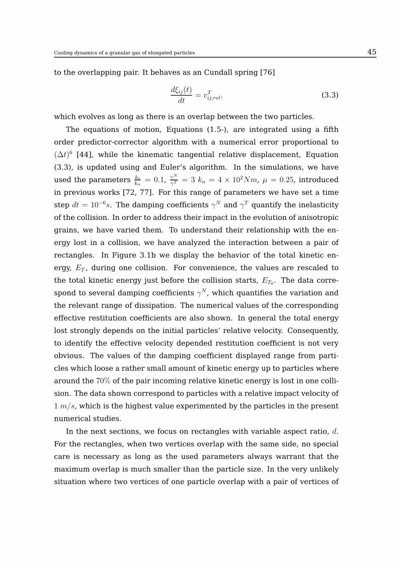
Cooling dynamics of a granular gas of elongated particles 45
to the overlapping pair. It behaves as an Cundall spring [76]
dξij(t)
dt= vTij,rel, (3.3)
which evolves as long as there is an overlap between the two particles.
The equations of motion, Equations (1.5-), are integrated using a fifth
order predictor-corrector algorithm with a numerical error proportional to
(∆t)6 [44], while the kinematic tangential relative displacement, Equation
(3.3), is updated using and Euler’s algorithm. In the simulations, we have
used the parameters ktkn
= 0.1, γN
γT = 3 kn = 4 × 10²Nm, µ = 0.25, introduced
in previous works [72, 77]. For this range of parameters we have set a time
step dt = 10−6s. The damping coefficients γN and γT quantify the inelasticity
of the collision. In order to address their impact in the evolution of anisotropic
grains, we have varied them. To understand their relationship with the en-
ergy lost in a collision, we have analyzed the interaction between a pair of
rectangles. In Figure 3.1b we display the behavior of the total kinetic en-
ergy, ET , during one collision. For convenience, the values are rescaled to
the total kinetic energy just before the collision starts, ET0 . The data corre-
spond to several damping coefficients γN , which quantifies the variation and
the relevant range of dissipation. The numerical values of the corresponding
effective restitution coefficients are also shown. In general the total energy
lost strongly depends on the initial particles’ relative velocity. Consequently,
to identify the effective velocity depended restitution coefficient is not very
obvious. The values of the damping coefficient displayed range from parti-
cles which loose a rather small amount of kinetic energy up to particles where
around the 70% of the pair incoming relative kinetic energy is lost in one colli-
sion. The data shown correspond to particles with a relative impact velocity of
1 m/s, which is the highest value experimented by the particles in the present
numerical studies.
In the next sections, we focus on rectangles with variable aspect ratio, d.
For the rectangles, when two vertices overlap with the same side, no special
care is necessary as long as the used parameters always warrant that the
maximum overlap is much smaller than the particle size. In the very unlikely
situation where two vertices of one particle overlap with a pair of vertices of
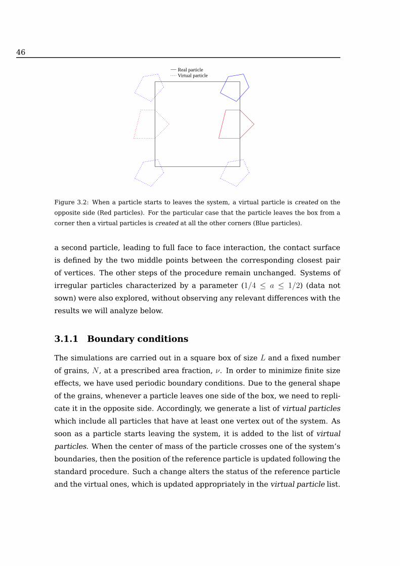
46
Real particleVirtual particle
Figure 3.2: When a particle starts to leaves the system, a virtual particle is created on the
opposite side (Red particles). For the particular case that the particle leaves the box from a
corner then a virtual particles is created at all the other corners (Blue particles).
a second particle, leading to full face to face interaction, the contact surface
is defined by the two middle points between the corresponding closest pair
of vertices. The other steps of the procedure remain unchanged. Systems of
irregular particles characterized by a parameter (1/4 ≤ a ≤ 1/2) (data not
sown) were also explored, without observing any relevant differences with the
results we will analyze below.
3.1.1 Boundary conditions
The simulations are carried out in a square box of size L and a fixed number
of grains, N , at a prescribed area fraction, ν. In order to minimize finite size
effects, we have used periodic boundary conditions. Due to the general shape
of the grains, whenever a particle leaves one side of the box, we need to repli-
cate it in the opposite side. Accordingly, we generate a list of virtual particles
which include all particles that have at least one vertex out of the system. As
soon as a particle starts leaving the system, it is added to the list of virtual
particles. When the center of mass of the particle crosses one of the system’s
boundaries, then the position of the reference particle is updated following the
standard procedure. Such a change alters the status of the reference particle
and the virtual ones, which is updated appropriately in the virtual particle list.
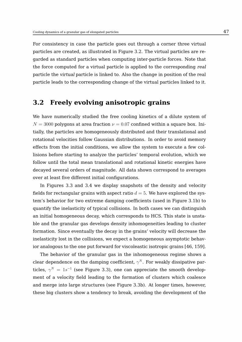
Cooling dynamics of a granular gas of elongated particles 47
For consistency in case the particle goes out through a corner three virtual
particles are created, as illustrated in Figure 3.2. The virtual particles are re-
garded as standard particles when computing inter-particle forces. Note that
the force computed for a virtual particle is applied to the corresponding real
particle the virtual particle is linked to. Also the change in position of the real
particle leads to the corresponding change of the virtual particles linked to it.
3.2 Freely evolving anisotropic grains
We have numerically studied the free cooling kinetics of a dilute system of
N = 3000 polygons at area fraction ν = 0.07 confined within a square box. Ini-
tially, the particles are homogeneously distributed and their translational and
rotational velocities follow Gaussian distributions. In order to avoid memory
effects from the initial conditions, we allow the system to execute a few col-
lisions before starting to analyze the particles’ temporal evolution, which we
follow until the total mean translational and rotational kinetic energies have
decayed several orders of magnitude. All data shown correspond to averages
over at least five different initial configurations.
In Figures 3.3 and 3.4 we display snapshots of the density and velocity
fields for rectangular grains with aspect ratio d = 5. We have explored the sys-
tem’s behavior for two extreme damping coefficients (used in Figure 3.1b) to
quantify the inelasticity of typical collisions. In both cases we can distinguish
an initial homogeneous decay, which corresponds to HCS. This state is unsta-
ble and the granular gas develops density inhomogeneities leading to cluster
formation. Since eventually the decay in the grains’ velocity will decrease the
inelasticity lost in the collisions, we expect a homogeneous asymptotic behav-
ior analogous to the one put forward for viscoleastic isotropic grains [46, 159].
The behavior of the granular gas in the inhomogeneous regime shows a
clear dependence on the damping coefficient, γN . For weakly dissipative par-
ticles, γN = 1s−1 (see Figure 3.3), one can appreciate the smooth develop-
ment of a velocity field leading to the formation of clusters which coalesce
and merge into large structures (see Figure 3.3b). At longer times, however,
these big clusters show a tendency to break, avoiding the development of the
48
(a)
(b)
(c)
Figure 3.3: Spatial evolution of a system with elongated particles d = 5 and a damping co-
efficient of γN = 1 s−1. The first column shows the screenshots of the system, the second
illustrates the velocity fields. The lighter the particles the faster they are. Pictures at t = 10 s
(a) , t = 100 s (b) and t = 200 s (c) are presented.
clustering instability (see Figure 3.3c), in agreement with the predictions for
viscoelastic grains [159, 172]. On the contrary, highly dissipative grains, with
γN = 103s−1, develop marked clusters of smaller sizes much faster, as can be
appreciated in Figure 3.4. Such clusters are correlated with the quick devel-

Cooling dynamics of a granular gas of elongated particles 49
(a)
(b)
(c)
Figure 3.4: (Color online) Spatial evolution a system with elongated particles d = 5 and a
damping coefficient of γN = 103s−1. The first column shows the screenshots of the system,
the second illustrates the velocity fields. The lighter the particles the faster they are. Pictures
at t = 10 s (a), t = 100 s (b) and t = 200 s (c) are presented.
opment of complex vortex structures in the grains’ velocity field. These well
defined, small clusters, tend to coalesce at larger times, although the over-
all process of large cluster development is severely slowed down when com-
pared to the evolution of weakly dissipative clusters. Increasing the particle
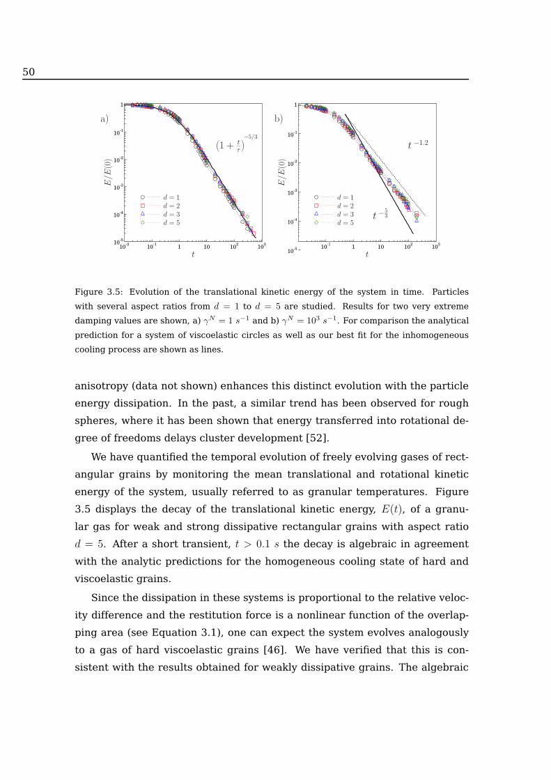
50
10-5
10-4
10-3
10-2
10-1
1
10-2
10-1
1 10 102
103
E/E
(0)
t
d = 1d = 2d = 3d = 5
(
1 + tτ
)
−5/3
a)
10-5
10-4
10-3
10-2
10-1
1
10-1
1 10 102
103
E/E
(0)
t
d = 1d = 2d = 3d = 5
t −1.2
t −53
b)
Figure 3.5: Evolution of the translational kinetic energy of the system in time. Particles
with several aspect ratios from d = 1 to d = 5 are studied. Results for two very extreme
damping values are shown, a) γN = 1 s−1 and b) γN = 103 s−1. For comparison the analytical
prediction for a system of viscoelastic circles as well as our best fit for the inhomogeneous
cooling process are shown as lines.
anisotropy (data not shown) enhances this distinct evolution with the particle
energy dissipation. In the past, a similar trend has been observed for rough
spheres, where it has been shown that energy transferred into rotational de-
gree of freedoms delays cluster development [52].
We have quantified the temporal evolution of freely evolving gases of rect-
angular grains by monitoring the mean translational and rotational kinetic
energy of the system, usually referred to as granular temperatures. Figure
3.5 displays the decay of the translational kinetic energy, E(t), of a granu-
lar gas for weak and strong dissipative rectangular grains with aspect ratio
d = 5. After a short transient, t > 0.1 s the decay is algebraic in agreement
with the analytic predictions for the homogeneous cooling state of hard and
viscoelastic grains.
Since the dissipation in these systems is proportional to the relative veloc-
ity difference and the restitution force is a nonlinear function of the overlap-
ping area (see Equation 3.1), one can expect the system evolves analogously
to a gas of hard viscoelastic grains [46]. We have verified that this is con-
sistent with the results obtained for weakly dissipative grains. The algebraic

Cooling dynamics of a granular gas of elongated particles 51
10-5
10-4
10-3
10-2
10-1
1
10-2
10-1
1 10 102
103
R/R
(0)
t
d = 1d = 2d = 3d = 5
t −2
a)
10-5
10-4
10-3
10-2
10-1
1
10-2
10-1
1 10 102
103
R/R
(0)
t
d = 1d = 2d = 3d = 5
t −2
b)
Figure 3.6: Evolution of the rotational energy of the system in time. Particles with several
aspect ratios from d = 1 upto d = 5 are studied.Results for two very extreme damping values
are shown, a) γN = 1 s−1 and b) γN = 103 s−1. For comparison the Haff’s analytical prediction
t−2. is also shown.
decay depicted in Figure 3.5a is characterized by the same exponent, β = −53,
analytically predicted for viscoelastic grains [46]. However, this is not the
case for highly dissipative grains, which cool down slower, with a character-
istic smaller exponent, β ≈ −1.2, in the algebraically decaying regime. It is
important to remark that the limitations of the used numerical scheme pre-
vented us to perform calculation with higher dissipative systems, for reaching
the hydrodynamic algebraic decay, E(t) ∼ t−1 limit [152].
On the other hand, for weakly dissipative systems, the decay of the transla-
tion kinetic energy also slows down at longer times. This can be attributed to
the development of stronger velocity correlations. Nevertheless, the narrow
time regime (system size effects) does not allow us to quantify the algebraic
dependence characteristic of the hydrodynamic regime, E(t) ∼ t−1 [152]. Con-
trary, the faster decay (t−53 ), which can be attributed to the dominance of big
clusters is quickly recovered. Larger system sizes will be required to iden-
tify the relevance of the intermediate regimes before reaching the asymptotic
state. For highly dissipative grains the smaller exponent, observed from very
short times, may suggest an earlier departure from HCS. In this case, the in-
terplay of cluster formation and break up with the development of large clus-

52
ters and their impact in the overall kinetic energy decay also remains to be
clarified. Nevertheless, Figure 3.5a and Figure 3.5b clearly indicate that nei-
ther the dissipation nor the shape does significantly modify the functional de-
pendence and the characteristic time scales in which the systems cool-down.
Moreover, analogous results (data not shown) are obtained for irregular parti-
cles with (1/4 ≤ a ≤ 1/2).
Figure 3.6 shows the decay of the rotational kinetic energy. After a short
transient, for t > 1 s, we observe an algebraic decay characterized by an
exponent −2 regardless of particle shape and inelasticity. This exponent,
in agreement with Haff’s law, can be understood assuming weak rotational-
translational correlations. The latter can be traced back to the fact that above
the Coulomb threshold, both the elastic and dissipative contributions of the
tangential force are linear functions of the lateral displacement and relative
velocity, respectively (see Equation 3.2). The deviations observed in E(t) at
longer times are much weaker for rotational kinetic energy, suggesting that ro-
tations are much less sensitive to the development of spatial inhomogeneities.
The different behavior in the decay of rotational and translational kinetic en-
ergy indicates a lack of energy equipartition during the whole cooling pro-
cess of the anisotropic grains, both in the homogeneous and inhomogeneous
regimes.
During the cooling process the velocity statistics was also examined (see
Figure 3.7a and Figure 3.7b). Starting from a Maxwellian speed distribu-
tion, the particle velocity distribution evolves with a scale characterized by the
mean translational kinetic energy. For weakly dissipative particles, which cool
down more uniformly over a wide range of times, it is reasonable to expect that
all the temporal dependence enters through the translational temperature and
we can then identify a dynamic scaling regime where the scaled velocity distri-
bution becomes stationary. Such a picture is consistent with the results shown
in Figure 3.7a, where we show the scaled speed distribution, P (c) (c = vv), at
the initial and final times. Regardless of the particle anisotropy, the distri-
bution shape remains close to a Maxwellian. For highly dissipative grains,
larger fluctuations are observed, although the shape remains also close to a
Maxwellian. In this case, one can argue that such a behavior arises as a result
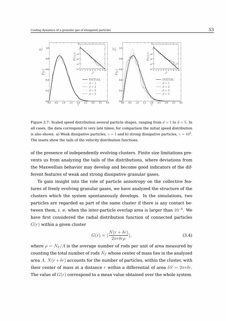
Cooling dynamics of a granular gas of elongated particles 53
0.0
0.2
0.4
0.6
0.8
1.0
0.0 0.5 1.0 1.5 2.0 2.5 3.0 3.5 4.0
10-4
10-3
10-2
10-1
1
10
0 1 2 3 4 5 6 7 8 9 10
P(c
)
c
P(c
)/c
c2
INITIALd = 1d = 2d = 3d = 5
a)
0.0
0.2
0.4
0.6
0.8
1.0
0.0 0.5 1.0 1.5 2.0 2.5 3.0 3.5 4.0
10-4
10-3
10-2
10-1
1
10
0 1 2 3 4 5 6 7 8 9 10
P(c
)
c
P(c
)/c
c2
INITIALd = 1d = 2d = 3d = 5
b)
Figure 3.7: Scaled speed distribution several particle shapes, ranging from d = 1 to d = 5. In
all cases, the data correspond to very late times; for comparison the initial speed distribution
is also shown. a) Weak dissipative particles, γ = 1 and b) strong dissipative particles, γ = 103.
The insets show the tails of the velocity distribution functions.
of the presence of independently evolving clusters. Finite size limitations pre-
vents us from analyzing the tails of the distributions, where deviations from
the Maxwellian behavior may develop and become good indicators of the dif-
ferent features of weak and strong dissipative granular gases.
To gain insight into the role of particle anisotropy on the collective fea-
tures of freely evolving granular gases, we have analyzed the structure of the
clusters which the system spontaneously develops. In the simulations, two
particles are regarded as part of the same cluster if there is any contact be-
tween them, i. e. when the inter-particle overlap area is larger than 10−6. We
have first considered the radial distribution function of connected particles
G(r) within a given cluster
G(r) = 〈N(r + δr)
2πrδrρ〉, (3.4)
where ρ = NT/A is the average number of rods per unit of area measured by
counting the total number of rodsNT whose center of mass lies in the analyzed
area A. N(r+ δr) accounts for the number of particles, within the cluster, with
their center of mass at a distance r within a differential of area δS = 2πrδr.
The value of G(r) correspond to a mean value obtained over the whole system.

54
In Figure 3.8, the radial distribution function of connected particles, G(r)
is illustrated for particles with different damping coefficients and variety of as-
pect ratios. At short distances, weakly dissipative grains display weak, short
range correlations characterized by the particle’s longest side, clearly visible
in Figure 3.8a. One can appreciate a correlation hole close to contact and
subsequently the radial distribution function develops a smooth peak whose
relative height decreases as the particle anisotropy increases. For strongly
dissipative particles the short range structure is markedly different, as shown
in Figure 3.8b. The inelasticity induces strong short range structures which
correspond to the different structures in which the particles can pack locally,
depending on their aspect ratio. The drawings in the figure indicate some of
the structures where one can find particles either perfectly aligned parallel
to each other along their long faces, or perpendicular to each other alternat-
ing long and short faces. This packing gives rise to clearly marked peaks,
whose positions change with the aspect ratio, d. The relative height of the
peaks also decrease with particle anisotropy, but in all cases their height are
larger than the corresponding particle anisotropies with smaller damping co-
efficient. This tendency to more marked close packed structures arise as a
combined effect of dissipation and alignment induced packing associated to
the particles shape. The insets of Figure 3.8 display the long distance decay
of the radial distribution function. The particle dissipation gives rise to larger
values of the radial distribution function at contact, but in both cases, and for
all the aspect ratios analyzed, we observe a long range decay, characteristic
of the development of long range clusters and structures. Such long range
structures have been observed in agitated isotropic grains as a result of long
range hydrodynamic correlations due to the lack of detailed balance in these
out of equilibrium systems [173].
Further information on the local structure of rod alignment is obtained
from the radial orientational distribution of connected particles within a given
cluster, Q(r), which can be defined as
Q(r) = 〈Qij〉 Qij = cos (2(θi − θj))δ(rij − r) (3.5)
where θi and θj are the angular orientation of particles i and its connected
neighbor j, at a distance rij. This distribution function provides quantita-

Cooling dynamics of a granular gas of elongated particles 55
0
1
2
3
4
5
6
1 2 3 4 5 6 7 8 9 10
0.0
1.0
2.0
3.0
4.0
40 80 120 160 200
G(r
)
r
d = 2d = 3d = 5
G(r
)
r
a)
0
1
2
3
4
5
6
7
8
9
10
1 2 3 4 5 6 7 8 9 10
0
2
4
6
8
10
40 80 120 160 200
G(r
)
r
d = 2d = 3d = 5
G(r
)
r
b)
Figure 3.8: Radial distribution function of connected particles obtained for system of particles
with aspect ratios from d = 2 to d = 5. Results for two very extreme damping values are
shown, a) γN = 1 s−1 and b) γN = 103 s−1, In both cases the particle alignment corresponding
to a few relevant peaks in the radial distribution function are drawn.
-0.4
-0.2
0.0
0.2
0.4
0.6
0.8
1.0
1 2 3 4 5 6 7 8 9 10
Q(r
)
r
d = 2d = 3d = 5
a)
-0.4
-0.2
0.0
0.2
0.4
0.6
0.8
1.0
1 2 3 4 5 6 7 8 9 10
Q(r
)
r
d = 2d = 3d = 5
b)
Figure 3.9: (Color online) Radial orientation distribution functions of connected particles,
Q(r), as defined in Equation 3.5 for system of particles with aspect ratios from d = 2 to d = 5.
Results for two very extreme damping values are shown, a) γN = 1 s−1 and b) γN = 103
s−1. In both cases the particle alignment corresponding to a few relevant peaks in the radial
orientation distribution function are drawn.
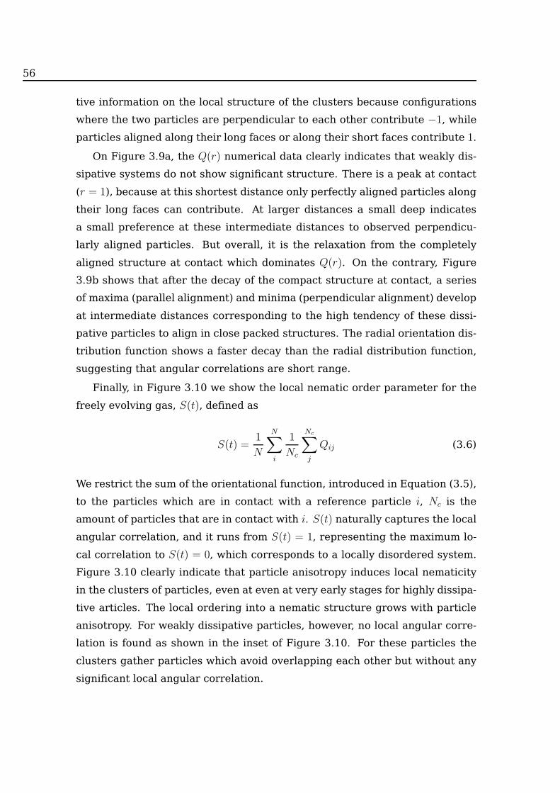
56
tive information on the local structure of the clusters because configurations
where the two particles are perpendicular to each other contribute −1, whileparticles aligned along their long faces or along their short faces contribute 1.
On Figure 3.9a, the Q(r) numerical data clearly indicates that weakly dis-
sipative systems do not show significant structure. There is a peak at contact
(r = 1), because at this shortest distance only perfectly aligned particles along
their long faces can contribute. At larger distances a small deep indicates
a small preference at these intermediate distances to observed perpendicu-
larly aligned particles. But overall, it is the relaxation from the completely
aligned structure at contact which dominates Q(r). On the contrary, Figure
3.9b shows that after the decay of the compact structure at contact, a series
of maxima (parallel alignment) and minima (perpendicular alignment) develop
at intermediate distances corresponding to the high tendency of these dissi-
pative particles to align in close packed structures. The radial orientation dis-
tribution function shows a faster decay than the radial distribution function,
suggesting that angular correlations are short range.
Finally, in Figure 3.10 we show the local nematic order parameter for the
freely evolving gas, S(t), defined as
S(t) =1
N
N∑
i
1
Nc
Nc∑
j
Qij (3.6)
We restrict the sum of the orientational function, introduced in Equation (3.5),
to the particles which are in contact with a reference particle i, Nc is the
amount of particles that are in contact with i. S(t) naturally captures the local
angular correlation, and it runs from S(t) = 1, representing the maximum lo-
cal correlation to S(t) = 0, which corresponds to a locally disordered system.
Figure 3.10 clearly indicate that particle anisotropy induces local nematicity
in the clusters of particles, even at even at very early stages for highly dissipa-
tive articles. The local ordering into a nematic structure grows with particle
anisotropy. For weakly dissipative particles, however, no local angular corre-
lation is found as shown in the inset of Figure 3.10. For these particles the
clusters gather particles which avoid overlapping each other but without any
significant local angular correlation.
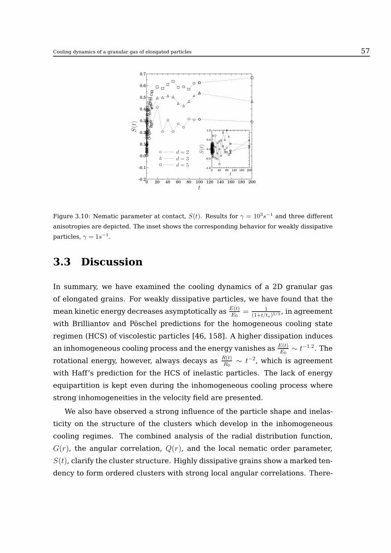
Cooling dynamics of a granular gas of elongated particles 57
-0.2
-0.1
0.0
0.1
0.2
0.3
0.4
0.5
0.6
0.7
0 20 40 60 80 100 120 140 160 180 200
-1.0
-0.5
0.0
0.5
1.0
0 40 80 120 160 200
S(t
)
t
d = 2d = 3d = 5
S(t
)
t
Figure 3.10: Nematic parameter at contact, S(t). Results for γ = 103s−1 and three different
anisotropies are depicted. The inset shows the corresponding behavior for weakly dissipative
particles, γ = 1s−1.
3.3 Discussion
In summary, we have examined the cooling dynamics of a 2D granular gas
of elongated grains. For weakly dissipative particles, we have found that the
mean kinetic energy decreases asymptotically as E(t)E0
= 1(1+t/to)5/3
, in agreement
with Brilliantov and Pöschel predictions for the homogeneous cooling state
regimen (HCS) of viscolestic particles [46, 158]. A higher dissipation induces
an inhomogeneous cooling process and the energy vanishes as E(t)E0∼ t−1.2. The
rotational energy, however, always decays as R(t)R0∼ t−2, which is agreement
with Haff’s prediction for the HCS of inelastic particles. The lack of energy
equipartition is kept even during the inhomogeneous cooling process where
strong inhomogeneities in the velocity field are presented.
We also have observed a strong influence of the particle shape and inelas-
ticity on the structure of the clusters which develop in the inhomogeneous
cooling regimes. The combined analysis of the radial distribution function,
G(r), the angular correlation, Q(r), and the local nematic order parameter,
S(t), clarify the cluster structure. Highly dissipative grains show amarked ten-
dency to form ordered clusters with strong local angular correlations. There-

fore, the system is nematogenic in this cooling process, and one can expect
that the observed clusters display a significant nematic order. The latter,
which increases with particle elongation, is very closely related to the typical
face to face interaction. The relevance of the interplay between particle shape
and inelasticity has been clearly appreciated by analyzing the structures of
weakly dissipative grains, where the local nematicity is essentially absent and
the density inhomogeneities are statistically much more isotropic. Our numer-
ical outcomes suggest that the strong dissipation and the particle anisotropy
induce the formation of ordered cluster structures and velocity vortices, which
notably slow down the cooling process and retard the appearance of large
clusters which break and reform. Increasing the particle anisotropy enhances
this distinct evolution as a function of the particle energy dissipation. This be-
havior can be attributed to the detailed interaction between ordered clusters
of particles, where rotational degrees of freedom play a relevant role. The
breakup of big clusters of elongated particles as a results of their collisions
leads to the formation of smaller clusters, promoting a faster decay of the
rotational kinetic energy. Such smaller clusters of ordered particles in turn
delay the development of the inhomogeneous cooling regime. Understanding
the impact of these strong correlations in agitated systems where energy is
supplied continuously constitutes an interesting venue in the fundamental un-
derstanding of the physics of anisotropic granulates and the subtle interplays
between particle shape and inelasticity.

Chapter 4
Stress distribution of faceted
particles in a silo after its partial
discharge
The design and exploitation of granular silos benefits from a detailed knowl-
edge of the mechanical properties of particle storages. In fact, a poor un-
derstanding of the impact that the grain properties has on granular deposits
necessary leads to a poor performance of the silo, both in terms of its stor-
age capabilities as well as its overall structural stability. Since the collective
behavior of such systems is not always easy to measure and control experi-
mentally, numerical modeling usually provides a very useful complementary
approach for understanding very complex processes like silo filling and dis-
charging [174–178].
In previous works, it was found the remarkable role that flat faces play
in the stress propagation of granular deposits [166, 179]. Elongation favors
rods’ alignment transverse to gravity, hindering stress transmission to the lat-
eral walls of the container. Then, as the particles increase their length, force
saturation becomes strongly reduced. On the contrary, squares tend to orient
with a diagonal parallel to gravity, transmitting the stress at π/4 with respect
to the gravity. This results in a clear saturation of the pressure with depth,
similar to what is observed in granular silos and known as Janssen’s effect.
In this chapter, we present a systematic theoretical and experimental co-
59

60
n
t
l1c
l2c
Figure 4.1: Photograph of the experimental setup of the two dimensional silo. On the right,
as example, there is a zoom of the d = 5.4 rods deposited in the bulk of the granular layer.
ordinated study of the structural and mechanical properties of packings of
faceted particles after their partial discharge from a silo. We show that par-
ticle shape and elongation has a profound effect on the process of silo dis-
charge and consequently, on the stress profiles developed. Hence, grain as-
pect ratio becomes a key parameter which controls the properties of pack-
ings of faceted particles within a silo. The simulations have been developed
by T. Kanzaki and R.C. Hidalgo in the framework of the project Estabilidad
y dinámica de medios granulares anisótropos (FIS2008-06034-C02-02). The
experiment have been conducted by researchers at University of Navarra in
the framework of the project Interacciones entre partículas y emergencia de
propiedades macroscópicas en medios granulares. (FIS2008-06034-C02-01)
4.1 Experiment
The experimental setup consists on a smooth, two dimensional silo filled either
with rods or square nuts (Figure 4.1). Two types of rods of 1.0mm diameter
have been used in this work. Both are monodisperse stainless steel rods with
different lengths: 2.4 and 5.4 mm. Hence, the aspect ratio of the rods is d = 2.4
and d = 5.4. It is important to note that the borders of the rods are truncated

Stress distribution of faceted particles in a silo 61
cones as explained in [179]. The square particles, d = 1, are DIN 557 nuts
3.16 mm wide and 6.9 mm side.
The container is built with two glass plates separated by two stainless-
steel strips 0.1 mm thicker than the particles so that the granular material is
confined in a mono-layer between the plates. The bottom of the silo is flat and
formed by two facing metal pieces whose edges touch each other. Since rods
and squares have different sizes, we have modified the container dimensions
correspondingly to generate analogous deposits. For rods (squares) the silo
is 180 mm (260 mm) wide and 790 mm (950 mm) high. The number of rods
necessary to fill the silo is larger than 5 × 10⁴ and 2 × 10⁴ for d = 2.4 and
d = 5.4 mm, respectively; while the number of required squares is around
5× 10³.
The granular sample is introduced through a hopper at the top of the silo by
pouring the grains homogeneously along the whole silo width. The feed rate
is measured to be around 200 particles per second for 2.4 mm rods, around 80
particles per second for 5.4 mm rods, and 70 particles per second for squares.
Once the deposit is generated, an orifice is opened at the silo bottom by sepa-
rating the two metal pieces that conform it. After a layer of rods (squares) of
around 250 mm (300 mm) has flowed out of the silo, the outlet is closed and the
flow is arrested. Then, the silo is completely emptied before a new realization
is performed. The outlet size is chosen to be small enough to stay away from
the silo lateral walls but big enough in order to guarantee the particle flow. At
this point, we remark that the flat faces of the particles provoke jams much
more frequently than in the case of the spheres [180]. Hence, the outlet sizes
selected have been 80 mm, 30 mm and 80 mm for square nuts, d = 2.4 rods
and d = 5.4 rods, respectively. In any case, it should be noted that, although
these dimensions may slightly affect some of the quantitative values obtained
in this work, the qualitative behavior remains unaltered.
A standard 10.2 megapixel camera is used to take pictures of the grains
inside the silo both after the filling and after the partial discharge. The region
recorded covers the whole width of the silo and a height going from 290 mm
to 410 mm for the case of the rods. For the case of the squares, the height
covered goes from 270 mm to 440 mm. In both cases we make sure that this

62
region is high enough to avoid the influence of the silo bottom. From the im-
ages, the particles are detected and their position and orientation determined.
In order to obtain good statistics we have performed 100 realizations for each
sample.
4.2 Model of 2D Spheropolygons
We have performed a Molecular Dynamics simulation of a two-dimensional
granular system composed of non-deformable dissipative particles, confined
within a rectangular box of width W . We have simulated 2×10⁴ rods of d = 2.4
and d = 5.4, even so 4×10³ squares. In order to generate deposits analogous to
the experimental ones, the system width is set toW = 180 mm (W = 172.8 mm)
for d = 2.4 (d = 5.4) and W = 276 mm for d = 1. The container boundaries
are composed of rigid particles, using one layer for each lateral wall, and two
particle layers at the bottom.
The particles are continuously added at the top of the box with a low feed
rate with random initial velocity and orientation. The granular media is de-
posited under the effect of gravity and it is let cool down until the particles’
mean kinetic energy is several orders of magnitude smaller than its initial
value. At this point, a hole of 80 mm, 36 mm and 80 mm for d = 1, d = 2.4
and d = 5.4 respectively, is opened at the middle-bottom of the container. The
orifice is closed when a grain located at the top-middle position of the hill,
marked as a reference, descends a prescribed vertical distance, s. The dis-
tance s takes the value of 300 mm for d = 1, 150 mm for d = 2.4, and 250 mm
for d = 5.4. After closing the container we let the system to cool down again
and the simulation finishes. To get good statistics, the results presented con-
stitute averages over at least twenty-four different repetitions for each case.
For calculating the particles interaction ~Fij we use a very efficient algo-
rithm proposed recently by Alonso-Marroquín et al [167, 181], allowing for
simulating a large number of particles. This numerical method is based on
the concept of spheropolygons, where the interaction between two contacting
particles only is governed by the overlap distance between them (see details
in [167, 181]). For defining the normal interaction FNij , we use a nonlinear

Stress distribution of faceted particles in a silo 63
Hertzian elastic force [182], proportional to the overlap distance of the parti-
cles. Moreover, to introduce dissipation, a velocity dependent viscous damp-
ing is assumed. Hence, the total normal force reads as
FNij = −kN · δ3/2 − γN · vNrel, (4.1)
where kN is the spring constant in the normal direction, γN is the damping
coefficient in the normal direction and ~vNrel is the normal relative velocity be-
tween i and j. The tangential force F Tij also contains an elastic term and the
tangential frictional term. Taking into account the Coulomb’s constraint it
reads as
F Tij = min{−kT · ξ − γT · |vTrel|, µFN
ij }, (4.2)
where γT is the damping coefficient on the tangential direction, vTrel is the
tangential component of the relative contact velocity of the overlapping pair.
ξ represents the elastic elongation of an imaginary spring at the contact [76],
which increases as dξ(t)/dt = vTrel as long as there is an overlap between the
interacting particles [76, 183]. µ accounts for the statical friction coefficient
of the particles.
The equations of motion are integrated using a fifth order predictor-corrector
algorithm with a numerical error proportional to (∆t)6 [44], while the kine-
matic tangential displacement, is updated using an Euler’s method. In order to
model hard particles, the maximum overlap must always be much smaller than
the particle size. This is ensured by introducing appropriate values for the nor-
mal and tangential elastic constants, which are set to ktkn
= 0.1, kn = 106N/m3/2.
together with the gravitational acceleration 10m/s2. For these parameters, the
time step should be around ∆t = 5 × 10⁻⁵s. Although the results we will de-
scribe are generic for hard particles, to achieve quantitative comparison with
experimental data we have carried out numerical simulations in which we
change both the normal damping coefficient and the static friction coefficient,
choosing the best fitting parameters. The damping coefficients are taken asνnνt
= 3, νt = 1 × 10²s−1 and µ = 0.5. Thus, we have ensured that the kinetic
energy loss and the dynamics of sediment formation are analogous to those
observed experimentally. It is important to remark that in all the simulations
reported below we do not change the particle’s material properties; only the

64
Figure 4.2: Packings of square nuts and simulated particles with d=1. Pictures of the experi-
ment (a) after the silo filling and (c) after the partial discharge. Numerical graphs (b) and (d)
on the same order.
particle aspect ratio has been varied.
4.3 Results
4.3.1 Packing Morphology
In [166, 179] we studied systematically the influence that the particle aspect
ratio has on the micro-mechanical properties of granular packing. Figure 4.2
shows the packings obtained for square particles, d = 1, both experimentally
and numerically. The granular columns resulting from the silo filling process
are presented in Figure 4.2a (exp) and Figure 4.2c (simul). Figure 4.2a con-
firms experimentally the tendency of square particles to align one of their
diagonals with gravity, as it was numerically predicted earlier [166].
We also describe in details the morphological and micro-mechanical changes,
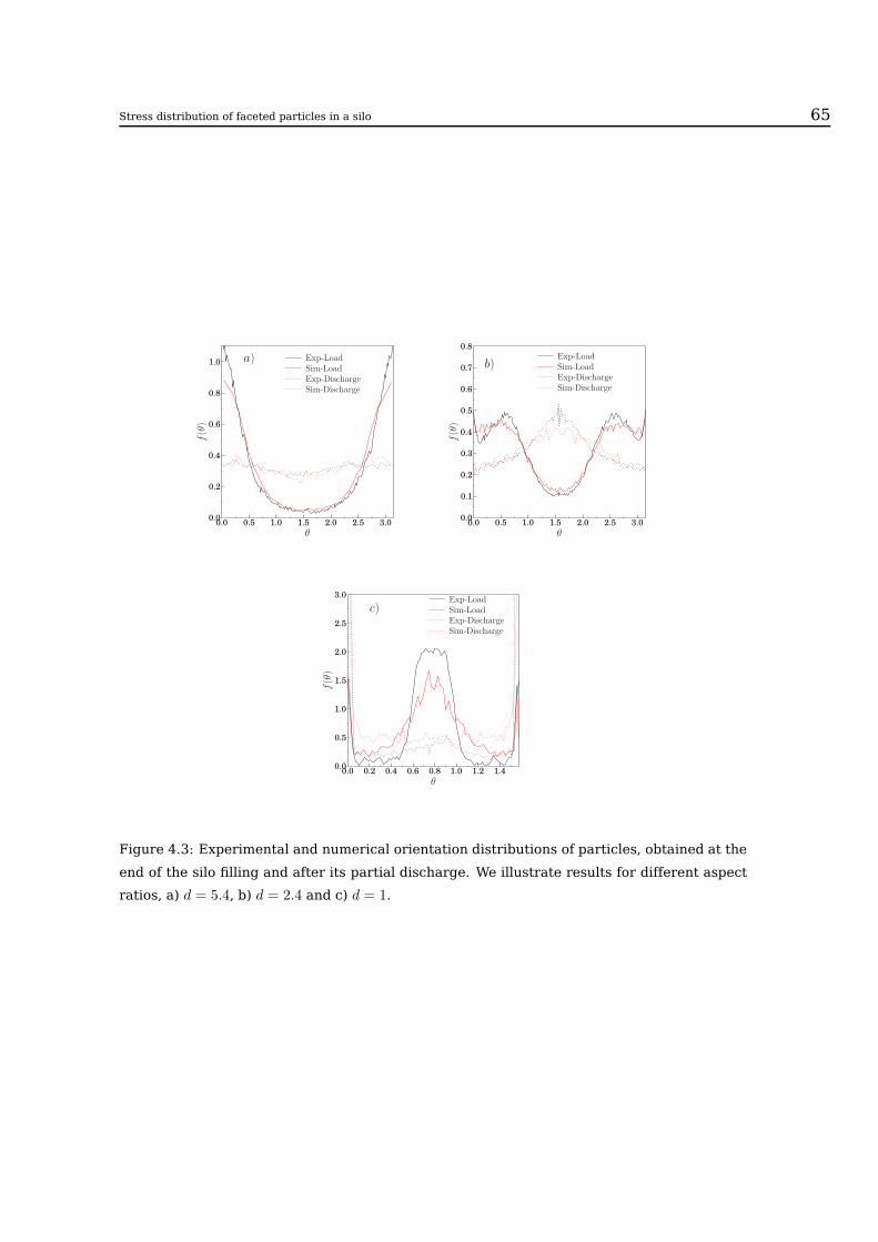
Stress distribution of faceted particles in a silo 65
0.0
0.2
0.4
0.6
0.8
1.0
0.0 0.5 1.0 1.5 2.0 2.5 3.0
f(θ
)
θ
Exp-LoadSim-LoadExp-DischargeSim-Discharge
a)
0.0
0.1
0.2
0.3
0.4
0.5
0.6
0.7
0.8
0.0 0.5 1.0 1.5 2.0 2.5 3.0
f(θ
)
θ
Exp-LoadSim-LoadExp-DischargeSim-Discharge
b)
0.0
0.5
1.0
1.5
2.0
2.5
3.0
0.0 0.2 0.4 0.6 0.8 1.0 1.2 1.4
f(θ
)
θ
Exp-LoadSim-LoadExp-DischargeSim-Discharge
c)
Figure 4.3: Experimental and numerical orientation distributions of particles, obtained at the
end of the silo filling and after its partial discharge. We illustrate results for different aspect
ratios, a) d = 5.4, b) d = 2.4 and c) d = 1.

66
which are induced by partial discharges in granular columns. The packing
morphology that results at the end of the partial discharge of the silo is illus-
trated in Figure 4.2b (exp) and Figure 4.2d (simul). It is noticeable that during
the discharge, the shear between grains induces their rotation and their set-
tlement in more stable mechanical states. Hence, the discharge induces an
alignment of the squares sides with gravity which minimizes the friction and
favors their vertical displacement.
The distributions, f(θ), of the particle orientation with respect to the direc-
tion transverse to gravity are analyzed. Figure 4.3 shows the particle distri-
butions obtained experimentally and numerically at the end of the silo filling
and after the silo partial discharge for three aspect ratios, d = 5.4, 2.4, and 1
(squares). The good agreement between the experimental and numerical re-
sults demonstrates the accuracy of our numerical simulation scheme. At the
end of the silo filling, elongated particles have a strong preference to align
horizontally (Figure 4.3a), in good agreement with previous results [184]. As
the rods become less asymmetric, particles develop a most probable orienta-
tion which decreases towards π/4 for the limiting case of squares. In this case,
it also becomes evident an important effect of the lateral walls which compete
with gravity and lead to a strong preference for parallel ordering of squares
in their vicinity. As a result, a distinct peak around θ = 0 and θ = π/2 can be
also identified in Figure 4.3.c. In sphere packings an analogous wall-induced
particle ordering, which can be significant in stress transmission, has been
previously reported [185, 186].
The packing morphology drastically changes at the end of the partial dis-
charge of the silo. For the case of rods (Figure 4.3a-b) the discharge induces
a decrease of the number of particles oriented horizontally and an increase
of the number of particles oriented vertically. This result may be a conse-
quence of the alignment of elongated particles with the flow streamlines. The
case of squares is completely different as it has been observed that they flow
more easily when one of their sides is aligned with gravity. This change in
the squares orientation, favored due to shearing forces with grains at rest,
leads to a distribution where a single peak is clearly observed at θ = 0 and
θ = π/2 (Figure 4.3c). We clarify below that this configuration minimizes the

Stress distribution of faceted particles in a silo 67
0.0
0.1
0.2
0.3
0.4
0.5
0.6
0.7
0.8
0.9
1.0
0 50 100 150 200 250x
Exp. Pπ4(x)
Sim. Pπ4(x)
Exp. Pπ2(x)
Sim. Pπ2(x)
a)
0.0
0.1
0.2
0.3
0.4
0.5
0.6
0.7
0.8
0.9
1.0
0 50 100 150 200 250x
Exp. Pπ4(x)
Sim. Pπ4(x)
Exp. Pπ2(x)
Sim. Pπ2(x)
b)
Figure 4.4: Experimental and numerical orientation of the squares for different sectors of the
silo a) at the end of the silo filling and b) after the silo partial discharge. Pπ
2(x) accounts for
the fraction of particles aligned mostly transversally to gravity, while Pπ
4(x) accounts for the
fraction of particles mostly aligned with gravity.
friction with the lateral neighboring particles and, consequently, the stress
transmission on the up-down direction is favored.
Although in the previous paragraphs we have analyzed the particle orien-
tation distribution by considering all the particles along the whole silo width,
it should be remarked that the partial silo discharge induces a spatial inhomo-
geneity in the horizontal direction. This effect is observed for all the aspect
ratios but it is specially dramatic for the case of squares. In Figure 4.4 we
quantify the internal structure analyzing the fraction of square particles which
align their side (diagonal) with gravity, at angles 0 < θ < π/8 and θ > π − π/8
(π/4 − π/8 < θ < π/4 + π/8), as a function to the distance to the left parallel
wall of the silo, Pπ2(x) (Pπ
4(x)). At the end of the filling process, most parti-
cles align their diagonals with gravity, except for a narrow region close to the
walls. After the partial discharge, it is evident that the fraction of squares with
a diagonal parallel to gravity is strongly depleted from the wall region, while
in the center, both groups of orientations are present with similar probability.
This result reflects what is observed by visual inspection of the discharge pro-
cess: a column of particles, limited by the orifice size, flows out the central
part of the silo. In the regions closer to the lateral walls the strong friction

68
between the moving particles and those at rest favors the growth of clusters
of squares with their sides aligned with the walls. This kind of flow is known
as ratholing, a characteristic and undesirable effect in silo discharge, where
stagnant zones are developed near the walls as only the particles above the
silo outlet are able to flow out [185].
4.3.2 Micromechanics
The study of the micromechanical properties of the granular packings will
provide more insight in the correlation between the deposit microstructure
and stress transmission. We can define the stress acting on a single particle
i in terms of Fci , the force it experiences due to its contact c. The local stress
tensor can be calculated as
σiαβ =
Ci∑
c=1
lci,αFci,β, (4.3)
where lci is the branch vector related to the contact c. The sum runs over all
contacts of particle i.
Figure 4.5 displays polar distributions of the stress tensor principal direc-
tions obtained for single particles (see Equation 4.3). We present results cor-
responding to columns of rods with d = 5.4 (a and b), and squares (c and d),
after loading (a and c) and after partial discharging (b and c). The data shown
correspond to an area of 100 mm wide at the center of the silo. In each plot,
the discontinuous arrows represent the largest (σ11) and smallest (σ22) eigen-
value of the mean stress tensor, within the whole studied area. The size of the
arrows is normalized with the size of the smallest eigenvalue. Note that at the
end of the silo filling process, the polar distribution for rods d = 5.4 displays
a strong preference for the transmission parallel to gravity (Figure 4.5a). On
the contrary, for squares, a clear symmetry is found in the distributions of the
two stress eigenvalues, evidencing that forces are mainly transmitted along
the π/4 and 3π/4 directions (Figure 4.5c). At the end of the partial discharge,
elongated rods keep the preference for vertical stress transmission, although
the stronger disorder in rod alignment favors a more isotropic stress distribu-
tion, leading to broader distributions of the stress eigenvalues (Figure 4.5b).

Stress distribution of faceted particles in a silo 69
σ22σ11
0
π/2
π/43π/4
π
5π/4
3π/2
7π/4a)
σ11
σ22
σ22σ11
0
π/2
π/43π/4
π
5π/4
3π/2
7π/4b)
σ11
σ22
σ22
σ11
0
π/2
π/43π/4
π
5π/4
3π/2
7π/4c)
σ11
σ22
σ22
σ11
0
π/2
π/43π/4
π
5π/4
3π/2
7π/4d)
σ11
σ22
Figure 4.5: Polar distribution of the principal directions of the local stress for elongated
particles with aspect ratio d = 5.4 (a) after the silo load and (b) after the partial discharge.
The same results for squares (c) after the load and (d) after the partial discharge.
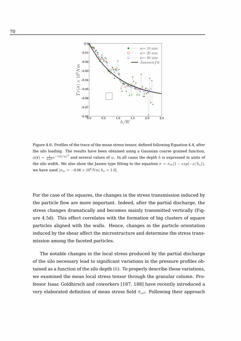
70
-0.08
-0.07
-0.06
-0.05
-0.04
-0.03
-0.02
-0.01
0.0
0.0 0.5 1.0 1.5 2.0 2.5
.
.
.
.
.
.....
.
.
....
....
.....
....
...
....
.......
.....
...
.....
..... .
Tr(σ)×10
6Nm
h/W
w= 10 mmw= 20 mmw= 40 mmJanssenfit
Figure 4.6: Profiles of the trace of the mean stress tensor, defined following Equation 4.4, after
the silo loading. The results have been obtained using a Gaussian coarse grained function,
φ(r) = 1πw2 e
−(|r|/w)2 and several values of w. In all cases the depth h is expressed in units of
the silo width. We also show the Jassen type fitting to the equation σ = σm(1 − exp(−x/hs)),
we have used [σm = −0.06× 10⁶Nm;hs = 1.0].
For the case of the squares, the changes in the stress transmission induced by
the particle flow are more important. Indeed, after the partial discharge, the
stress changes dramatically and becomes mainly transmitted vertically (Fig-
ure 4.5d). This effect correlates with the formation of big clusters of square
particles aligned with the walls. Hence, changes in the particle orientation
induced by the shear affect the microstructure and determine the stress trans-
mission among the faceted particles.
The notable changes in the local stress produced by the partial discharge
of the silo necessary lead to significant variations in the pressure profiles ob-
tained as a function of the silo depth (h). To properly describe these variations,
we examined the mean local stress tensor through the granular column. Pro-
fessor Isaac Goldhirsch and coworkers [187, 188] have recently introduced a
very elaborated definition of mean stress field σαβ. Following their approach

Stress distribution of faceted particles in a silo 71
-0.035
-0.03
-0.025
-0.02
-0.015
-0.01
-0.005
0.0
0.0 0.5 1.0 1.5 2.0 2.5 3.0 3.5 4.0
............
..
..
.. .
Tr(σ)×10
6Nm
h/W
CentreRight WallLeft Wall
a)
-0.03
-0.025
-0.02
-0.015
-0.01
-0.005
0.0
0.0 0.5 1.0 1.5 2.0 2.5 3.0
..
...
...
..
..
.
.Tr(σ)×10
6Nm
h/W
CentreRight WallLeft Wall
b)
Figure 4.7: Profiles of the trace of the mean stress tensor (pressure) after the load a) and the
partial discharge b) for rods with d = 5.4. In all cases the depth h is expressed in units of the
silo width.
the stress σαβ(r) at point r, is given by the expression
σαβ(~r) =1
2
∑
i,j;i 6=j
fijαrijβ
∫ 1
0
ds φ[~r − ~ri + s~rij ], (4.4)
where the sum runs over all the contacting particles i, j, whose center of mass
are at ~ri and ~rj, respectively. Moreover, ~fij accounts for the force exerted by
particle j on particle i and ~rij ≡ ~ri − ~rj. The coarse grained (CG) function,
φ(~R), is positive semidefinite normalized function, with a single maximum at
R = 0. In our case, we used a Gaussian coarse function, φ(r) = 1πw2 e
−(|r|/w)2,
where the sign convention is that compressive stress is negative. The value of
w defines the coarse grained scale. We note that the data was also evaluated
using less sophisticated mean stress definitions [189, 190] and very similar
results came out (data not shown).
To clarify the effect of the CG scale w on the results, we evaluate the nu-
merical data for several values of w. The stress tensor components –defined
by Equation 4.4– were calculated within specific areas and the contribution of
the contacts within the selected area is weighted by the function φ(r). Hence,
the size of the working area is controlled by the size of the CG scale w. Specif-
ically, the trace of stress tensor (pressure) obtained for a silo of squares was

72
-0.06
-0.05
-0.04
-0.03
-0.02
-0.01
0.0
0.0 0.5 1.0 1.5 2.0 2.5
.......
...
..
..
. .Tr(σ)×10
6Nm
h/W
CentreRight WallLeft Wall
a)
-0.03
-0.025
-0.02
-0.015
-0.01
-0.005
0.0
0.0 0.2 0.4 0.6 0.8 1.0 1.2 1.4 1.6
.....
..
.. .
Tr(σ)×10
6Nm
h/W
CentreRight WallLeft Wall
b)
Figure 4.8: Profiles of the trace of the mean stress tensor (pressure) after the load a) and the
partial discharge b) for squares. In all cases the depth h is expressed in units of the silo width.
examined in Figure 4.6. Note that the depth of the silo has been normalized
with the width of the deposit x = h/W . Moreover, for comparison, the numer-
ical fit using a Janssen-type formula σ = σm(1 − exp(−x/hs)), are also shown
[191, 192].
Here, the magnitude of σm represents the saturation stress and hs indicates
the characteristic value of depth at which the pressure on the column surface
stabilizes. The pressure profiles were calculated fixing the horizontal coordi-
nate and varying the vertical one (up-down) in units of w. The results reveal
that stress fluctuations at fixed depth vanish when increasing the value of w.
This indicates the existence of a CG scale for which the stress tensor field
is resolution independent [187, 188]. The data presented below have been
carefully evaluated for different values of w. Provided that the stress profiles
are not homogeneous due to the action of the gravity field, we have carefully
chosen the value of w to accurately capture the spatial stress variation.
In Figures 4.7 and 4.8, we display the trace of the mean stress tensor for
rods d = 5.4 and squares, respectively. In all cases, a coarse grained distance
of w = 40mm was used for the calculation of the mean stress tensor. This value
is approximately six and seven times larger than particle size of the squares
and the rods of d = 5.4, respectively. As we pointed out earlier, after the silo

Stress distribution of faceted particles in a silo 73
loading with elongated particles, the stress is transmitted preferentially par-
allel to gravity. As a result, the weak stress transmission on the horizontal
direction hinders pressure saturation, which is not completely reached for the
system sizes studied here (Figure 4.7a). The pressure profiles are very similar
both in the center of the column and in the region close to the walls. After
the partial discharge (Figure 4.7b), notable modifications are induced on the
trace of the mean stress tensor. On the center of the silo, the larger disorder
in particle orientation enhances the stress transmission in the horizontal di-
rection which is typically associated to pressure saturation. Effectively, when
we approach to the bottom of the silo the pressure first reaches a maximum
and then, it decreases at the very bottom. This pressure reduction denotes
arch formation in the region near the outlet. In the region close to the walls
the pressure increases with h until the bottom of the silo, probably due to
horizontal rod alignment induced by the bottom.
For squares (Figure 4.8a), the opposite scenario holds true. After filling the
silo, in the central part of the column the force is transmitted preferentially
at π/4 with respect to gravity, providing an efficient mechanism to channel
stresses towards the lateral walls. Accordingly, a saturation in the pressure
profile seems to be observed. However, close to the walls the strong face
to face interaction induces the particle alignment and, consequently, a linear
pressure profile is developed. The scenario is altered by the discharge of the
square nuts which become preferentially aligned with the silo walls even in the
center part of the column. This vertical alignment results in a stress transfer
to the bottom of the silo which makes pressure saturation hardly visible.
4.4 Conclusions
In this work we have shown that the partial discharge of a silo filled with
faceted grains has a profound effect on the deposit morphology and its stress
distribution. During the discharge, the shear between grains induces their
rotation and their settlement in more disordered arrangements. For elon-
gated particles, the preferred horizontal orientation displayed after the silo
filling disappears. For square particles, the discharge provokes an alignment
of their sides with gravity which minimizes the friction and favors their verti-
cal displacement. Such a structure leads to ratholing, a flow pattern which is
typically associated to cohesive effects, but that here, we show that it can also
be induced by the geometrical properties of the particles.
As a result of the changes in particle orientation, the pressure distribution
in the silo changes qualitatively; while for elongated rods lateral stress trans-
mission is promoted by the enhanced disorder leading to a faster pressure
saturation, the opposite holds for squares. In this latter case the alignment of
squares induced by the flow destroys the initial force chain network which is
replaced by a mainly vertical stress transmission. As a consequence, a signifi-
cant reduction of the pressure saturation effect is observed.
With the results reported here, we attempt to clarify the performance and
stability of silos, which need to support high stresses that become very sensi-
tive to grain shapes and the silo steering history. If we increase the amount of
material flowing out of the silo, or induce a second discharge, we expect that
the observed effect will be enhanced. Although we have focused on weakly
disordered initial deposits, due to the low feeding rates used to fill the silo,
the main features discussed here are expected for other silo filling proce-
dures. Perhaps, increasing the disorder of the initial packing will generically
decrease the relative magnitude of the changes discussed.
Chapter 5
Granular packings of cohesive
elongated particles
Very often, loose and disordered granular structures appear in many tech-
nological processes and even everyday life. They can be found in collapsing
soils [193–196], fine powders [197–199] or complex fluids [200, 201]. Gener-
ally, those fragile grain networks are correlated with the presence of cohesive
forces [197, 202–204]. Typical fine powders have in most cases an effective
attractive force, e.g. due to a capillary bridge between the particles or van der
Waals forces (important when going to very small grains, e.g. nano-particles).
This force is known to be of great importance, e.g. for the mechanical behavior
and the porosity of the macroscopic material [205–208]. This cohesive force
leads also to the formation of loose and fragile granular packings as investi-
gated in detail for structures generated by successive deposition of spherical
grains under the effect of gravity [202, 203, 205, 209].
The main objective of this chapter is to clarify the effect that an effective
attractive force has on the packing properties of elongated grains. Here we
focus on packings generated by deposition under gravity.
5.1 2D spheropolygons with cohesion
We have performed Discrete Element Modeling of a two-dimensional gran-
ular system composed of non-deformable oval particles, i.e. spheropolygons
75

76
Figure 5.1: Simulated packings of elongated cohesive particles settled by gravity. Final config-
urations are shown for the same granular bond number Bog = 104 and increasing elongation:
(a) d = 2, (b) d = 3, (c) d = 5 and (d) d = 10.

Granular packings of cohesive elongated particles 77
[167, 181] composed of two lines of equal length and two half circles of same
diameter. The width of a particle is the smaller diameter, given by the dis-
tance between the two lines (equals the circle diameter), whereas the length
is the maximum extension. The aspect ratio d is defined by the length di-
vided by width. This system is confined within a rectangular box of width W .
Its lateral boundaries as well as the bottom are each built of one very long
spheropolygonal particle, which is fixed. In order to generate analogous de-
posits, the system width is always set toW = 20×d (in units of particle width).
As illustrated in Figure 5.1 the particles are continuously added at the top of
the box with very low feed rate and a random initial velocity and orientation.
The granular system settles under the effect of gravity and is relaxed until the
particles’ mean kinetic energy is several orders of magnitude smaller than its
initial value.
For calculating the particles’ interaction ~Fij we use a very efficient algo-
rithm proposed recently by Alonso-Marroquín et al [167, 181], allowing for
simulating a large number of particles. This numerical method is based on
the concept of spheropolygons, where the interaction between two contacting
particles only is governed by the overlap distance between them (see details
in References [167, 181]).
To define the normal interaction FNij , we use a nonlinear Hertzian elastic
force [182], proportional to the overlap distance δ of the particles. Moreover,
to introduce dissipation, a velocity dependent viscous damping is assumed.
Hence, the total normal force reads as FNij = −kN · δ3/2 − γN · vNrel, where kN
is the spring constant in the normal direction, γN is the damping coefficient
in the normal direction and vNrel is the normal relative velocity between i and
j. The tangential force F Tij also contains an elastic term and a tangential fric-
tional term accounting also for static friction between the grains. Taking into
account Coulomb’s friction law it reads as, F Tij = min{−kT · ξ− γT · |vTrel|, µFN
ij },where γT is the damping coefficient in tangential direction, vTrel is the tan-
gential component of the relative contact velocity of the overlapping pair. ξ
represents the elastic elongation of an imaginary spring with spring constant
kT at the contact [76], which increases as dξ(t)/dt = vTrel as long as there is an
overlap between the interacting particles [76, 183]. µ is the friction coefficient

78
of the particles.
Additionally, here we consider bonding between two particles in terms of
a cohesion model with a constant attractive force Fc acting within a finite
range dc. Hence, it is expected that the density and the characteristics of the
density profiles are determined by the ratio between the cohesive force Fc and
gravity Fg = mg, typically defined as the granular Bond number Bog = Fc/Fg.
Thus, the case of Bog = 0 corresponds to the cohesion-less case whereas for
Bog →∞ gravity is negligible.
The equations of motion, Equations (1.5-3.1) are integrated using a fifth or-
der predictor-corrector algorithm with a numerical error proportional to (∆t)6
[44], while the kinematic tangential displacement, is updated using an Euler’s
method. In order to model hard particles, the maximum overlap must always
be much smaller than the particle size; this is ensured by introducing values
for normal and tangential elastic constants, kT/kN = 0.1, kN = 103N/m3/2.
The ratio between normal and tangential damping coefficients is taken as
γN/γT = 3, γT = 1 × 10²s−1 while gravity is set to g = 10 m/s2 and the co-
hesion range to dc = 0.0001 (in units of particle width) to account for a very
short range attraction, as mediated, e.g. by capillary bridges or van der Waals
force. For these parameters, the time step should be around ∆t = 5× 10⁻⁶s.
In all the simulations reported here, we have kept the previous set of pa-
rameters and only the particle aspect ratio and the Bond number Bog have
been modified. We have also carried out additional runs (data not shown) us-
ing other particles’ parameters, and we have verified that the trends and prop-
erties of the quantities we subsequently analyze are robust to such changes.
5.2 Results and discussion
We systematically study granular deposits of particles with aspect ratio from
d = 2 to d = 10 and different Bond numbers. In all simulations presented here
we have used 6 × 10³ rods. In Figure 5.1 we illustrate the granular packings
obtained for several particle shapes and constant Bond number Bog = 104. De-
spite of the presence of a gravity field acting downwards, the formation of very
loose and disordered granular structures is very noticeable. Moreover, as the
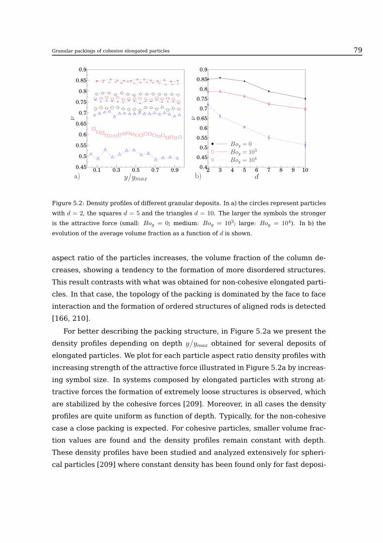
Granular packings of cohesive elongated particles 79
0.45
0.5
0.55
0.6
0.65
0.7
0.75
0.8
0.85
0.9
0.1 0.3 0.5 0.7 0.9
ν
y/ymaxa)0.4
0.45
0.5
0.55
0.6
0.65
0.7
0.75
0.8
0.85
0.9
2 3 4 5 6 7 8 9 10
. . ..
.
.
ν
d
Bog = 0
Bog = 103
Bog = 104
b)
Figure 5.2: Density profiles of different granular deposits. In a) the circles represent particles
with d = 2, the squares d = 5 and the triangles d = 10. The larger the symbols the stronger
is the attractive force (small: Bog = 0; medium: Bog = 103; large: Bog = 104). In b) the
evolution of the average volume fraction as a function of d is shown.
aspect ratio of the particles increases, the volume fraction of the column de-
creases, showing a tendency to the formation of more disordered structures.
This result contrasts with what was obtained for non-cohesive elongated parti-
cles. In that case, the topology of the packing is dominated by the face to face
interaction and the formation of ordered structures of aligned rods is detected
[166, 210].
For better describing the packing structure, in Figure 5.2a we present the
density profiles depending on depth y/ymax obtained for several deposits of
elongated particles. We plot for each particle aspect ratio density profiles with
increasing strength of the attractive force illustrated in Figure 5.2a by increas-
ing symbol size. In systems composed by elongated particles with strong at-
tractive forces the formation of extremely loose structures is observed, which
are stabilized by the cohesive forces [209]. Moreover, in all cases the density
profiles are quite uniform as function of depth. Typically, for the non-cohesive
case a close packing is expected. For cohesive particles, smaller volume frac-
tion values are found and the density profiles remain constant with depth.
These density profiles have been studied and analyzed extensively for spheri-
cal particles [209] where constant density has been found only for fast deposi-

80
0.0
0.1
0.2
0.3
0.4
0.5
0.6
0.7
0.8
0.9
1.0
0.0 0.5 1.0 1.5 2.0 2.5 3.0
..................
.........
..........................
..........
.............
.......
.......
.
f(θ)
θ
Bog = 0
Bog = 103
Bog = 104
a)
0.0
0.5
1.0
1.5
2.0
2.5
3.0
3.5
0.0 0.5 1.0 1.5 2.0 2.5 3.0
......................................................................
....................
.
f(θ)
θ
Bog = 0
Bog = 103
Bog = 104
b)
Figure 5.3: Orientation distributions of particles for two aspect ratios, a) d = 2 and b) d = 10.
In each case, results for several bond numbers are presented.
tion as strongly influenced by inertia. However, an extremely slow and gentle
deposition process, allowing for relaxation of the deposit due to its own weight
after each deposition, leads to a decreasing density with vertical position. Ob-
viously, here the feed rate is not sufficiently slow. Additionally, as particles are
added at the top they are accelerated before, thus reaching the deposit with a
non negligible impact velocity.
Complementary, in Figure 5.2b a systematic study of the global volume
fraction depending on the particle aspect ratio is presented for different bond
numbers. All curves show the overall trend of decreasing density with increas-
ing aspect ratio d. For packings of non-cohesive particles disordered and thus
substantially looser structures can only be found with very large aspect ratio
as found earlier numerically and experimentally [166, 179]. For very cohe-
sive particles (see Figure 5.1), however, loose and disordered granular struc-
tures can be easily stabilized, leading to much lower densities independent on
shape/elongation. This is notably enhanced as the aspect ratio of the parti-
cles increases and, consequently, the volume fraction of the packings quickly
decreases.
In order to characterize the packing morphology, we examine the orienta-
tions of the particles. In Figure 5.3, the distributions of particle’s orientation

Granular packings of cohesive elongated particles 81
f(θ), with respect to the horizontal direction, for rods with aspect ratio d = 2
and d = 10 are illustrated. We present results for several bond numbers.
First, for the non-cohesive case, the geometry of the particle dominates the
final structures of the compacted piles. Note that at the end of the deposi-
tion process, long particles (d = 10) most probably lie parallel to the substrate
(θ = 0 and θ = π), while the most unlikely position corresponds to standing
rods (θ = π2). Nevertheless, as the aspect ratio decreases, there is a shift in
the most probable orientation, leading to a peaked distribution at an interme-
diate orientation [166, 179]. Furthermore, this shift of the maximum is not
observed for highly cohesive particles. In general, as the strength of the at-
tractive force gets stronger, the final packing tends to a flatter distribution. As
we pointed out earlier, very elongated particles with strong attractive forces
form extremely loose structures. As the aspect ratio gets higher, the rods
form highly jammed and disordered networks because during the deposition
local particle rearrangements are constrained by the attractive force. The lat-
ter, is corroborated by the distribution of the angular orientation, where now
the probability for standing rods which was zero in the non-cohesive case is
enhanced with increasing bond number (Figure 5.3b). It seems that, for suffi-
ciently large aspect ratio d, there is a threshold bond number needed to have
a non-zero probability for standing rods.
The packing morphology is also examined through a radial orientation
function Q(r), defined as
Q(r) = 〈cos (2(θi − θj))δ(rij − r)〉 (5.1)
where θi and θj are the angular orientations of particles i and j, respectively.
Q(r) accounts for the mean value of the angular correlation between a given
particle i and a particle j with their center of mass at a distance rij. Note
that, this distribution function provides useful quantitative information on the
local morphology of the rod packings. Configurations where the two rods are
perpendicular to each other contribute −1 to Q(r), while rods aligned along
their long faces or along their short faces contribute with 1 [166, 179].
In Figure 5.4a and Figure 5.4b the numerical data for packing of cohesive
particles with aspect ratio d = 2 and d = 5 are shown for comparison. Both fig-
ures show a series of maxima (parallel alignment) and minima (perpendicular

82
-0.6
-0.4
-0.2
0.0
0.2
0.4
0.6
0.8
1.0
1 2 5 10
Q(r)
r
Bog = 0
Bog = 103
Bog = 104
a)
0.0
0.2
0.4
0.6
0.8
1.0
1 2 5 10
Q(r)
r
Bog = 0
Bog = 103
Bog = 104
b)
Figure 5.4: Radial orientation distribution functions, Q(r), as defined in Equation 5.1 for rod
deposits with two different aspect ratios, a) d = 2 and b) d = 5. In each case, results for
several Bond numbers are presented. At specific maxima/minima the corresponding particle
configurations are illustrated.
P(φ) Bog=0
P(φ) Bog=10
4
0
π/2
π/43π/4
π
5π/4
3π/2
7π/4
Figure 5.5: Polar distribution of the principal direction (larger eigenvalue of the stress tensor
for each particle σαβ), obtained for particles with d = 10. For comparison, the data for Bog = 0
and Bog = 104 is presented.
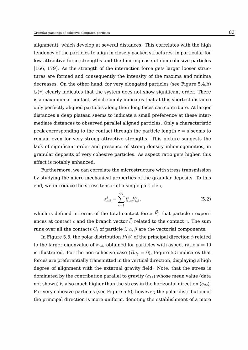
Granular packings of cohesive elongated particles 83
alignment), which develop at several distances. This correlates with the high
tendency of the particles to align in closely packed structures, in particular for
low attractive force strengths and the limiting case of non-cohesive particles
[166, 179]. As the strength of the interaction force gets larger looser struc-
tures are formed and consequently the intensity of the maxima and minima
decreases. On the other hand, for very elongated particles (see Figure 5.4.b)
Q(r) clearly indicates that the system does not show significant order. There
is a maximum at contact, which simply indicates that at this shortest distance
only perfectly aligned particles along their long faces can contribute. At larger
distances a deep plateau seems to indicate a small preference at these inter-
mediate distances to observed parallel aligned particles. Only a characteristic
peak corresponding to the contact through the particle length r = d seems to
remain even for very strong attractive strengths. This picture suggests the
lack of significant order and presence of strong density inhomogeneities, in
granular deposits of very cohesive particles. As aspect ratio gets higher, this
effect is notably enhanced.
Furthermore, we can correlate the microstructure with stress transmission
by studying the micro-mechanical properties of the granular deposits. To this
end, we introduce the stress tensor of a single particle i,
σiαβ =
Ci∑
c=1
lci,αFci,β, (5.2)
which is defined in terms of the total contact force ~F ci that particle i experi-
ences at contact c and the branch vector ~lci related to the contact c. The sum
runs over all the contacts Ci of particle i, α, β are the vectorial components.
In Figure 5.5, the polar distribution P (φ) of the principal direction φ related
to the larger eigenvalue of σαβ, obtained for particles with aspect ratio d = 10
is illustrated. For the non-cohesive case (Bog = 0), Figure 5.5 indicates that
forces are preferentially transmitted in the vertical direction, displaying a high
degree of alignment with the external gravity field. Note, that the stress is
dominated by the contribution parallel to gravity (σ11) whose mean value (data
not shown) is also much higher than the stress in the horizontal direction (σ22).
For very cohesive particles (see Figure 5.5), however, the polar distribution of
the principal direction is more uniform, denoting the establishment of a more

84
-3000
-2500
-2000
-1500
-1000
-500
0
0.0 0.5 1.0 1.5 2.0 2.5 3.0
....
..
...
. .
Tr(
¯σαβ)
h/W
Bog = 0
Bog = 104
Jansen− Fit− 1Jansen− Fit− 2
Figure 5.6: Profiles of the trace of the mean stress tensor, obtained for particles with d = 10
and two different bond numbers. The depth is normalized with the width W of the system.
We also show the fitting to the equation σ = σm(1 − exp(−x/hs)), where we used [σm =
2500N/m;hs/W = 1.2] and [σm = 4800N/m;hs/W = 2.2] for case 1 and 2, respectively.
spherical stress state. Hence, in this case the stress is more isotropically
transmitted while the alignment with the external gravity field diminishes.
This effect correlates with the formation of very loose packings and the lack
of significant order and the presence of strong density inhomogeneities.
Finally, we show that the changes in microstructure induced both by par-
ticle geometry and the attractive force lead to significant modifications in the
pressure (trace of the mean stress tensor) profiles as a function of the silo
depth h. The mean stress tensor, σαβ, can be calculated for a given represen-
tative volume element (RVE) with area ARVE resulting in
σαβ =1
ARVE
N∑
i=1
wvσiαβ . (5.3)
The sum runs over the representative volume element while wv is an appropri-
ate average weight. Although recently Professor Isaac Goldhirsch and cowork-
ers have developed a very accurate procedure for calculating wv and σαβ
[188, 211], for simplicity’s sake we use particle-center averaging and choose
the simplest weighting: wv = 1 if the center of the particle lies inside the

Granular packings of cohesive elongated particles 85
averaging area ARVE and wv = 0 otherwise [189, 190].
In Figure 5.6, we display the trace of the mean stress tensor, defined fol-
lowing Equation 5.3, for elongated particles with d = 10. For the calculation
of the mean stress tensor we have used a representative volume element with
a size equivalent to five particle lengths ARVE = 5d × 5d. The depth has been
normalized with the width of the deposit x = h/W . Moreover, for comparison,
the numerical fit using a Janssen-type formula σ = σm(1−exp(−x/hs)), are also
shown. Here, the magnitude of σm represents the saturation stress and hs in-
dicates the characteristic value of depth at which the pressure in the deposit
stabilizes.
As we have mentioned earlier, non-cohesive elongated particles transmit
stress preferentially parallel to gravity. As a result, the weak transmission
to the the lateral walls weakens pressure saturation (Figure 5.6), which is
reflected by the large saturation depth hs and stress σm. The latter is conse-
quence of the horizontal alignment of the flat faces of the rods, which induces
an anisotropic stress transmission, from top to bottom. However, the scenario
changes drastically for very cohesive particles. As we also pointed out earlier,
when the attractive force is increased, particle orientations deviate from the
horizontal and a larger disorder in the particle orientation distribution shows
up. As a result, the spherical component of the local stress is notably enhanced
with respect to the deviatoric part, which is related to the gravity direction.
Hence, for very cohesive particles Bo = 104 of d = 10 we found notably smaller
values of saturation depth hs and stress σm. In this respect, introducing an
attractive force has a very similar effect as reducing the particle elongation.
5.3 Conclusions
We have shown that introducing an attractive force in deposits of elongated
grains has a profound effect on the deposit morphology and its stress profiles.
In deposits of non-cohesive particles the topology is dominated by the forma-
tion of ordered structures of aligned rods. Elongated particles tend to align
horizontally and the stress is mainly transmitted from top to bottom, reveal-
ing an asymmetric distribution of the local stress. Lateral force transmission

becomes less favored compared to vertical transfer, thus hindering pressure
saturation with depth. For deposits of cohesive particles, the preferred hori-
zontal orientation is less pronounced with increasing cohesion. Very elongated
particles with strong attractive forces form extremely loose structures, char-
acterized by orientation distributions, which tend to a uniform behavior when
increasing the Bond number. As a result of these changes, the pressure distri-
bution in the deposits changes qualitatively. The spherical component of the
local stress is notably enhanced with respect to the deviatoric part. Hence,
the lateral stress transmission is promoted by the enhanced disorder and it
leads to a faster pressure saturation with depth.

Chapter 6
CUDA
Nowadays, molecular dynamics is widely accepted as an effective method for
addressing physical and engineering issues concerning dense granular media.
This method is generally distinguished by the inclusion of several degrees-of-
freedom as well as state-full contact. Moreover, it is also suitable for describ-
ing complicated particle shapes (non-sphericity) and polydisperse systems.
Nevertheless, the main disadvantages of molecular dynamics algorithms,
implemented on computing processing units (CPU), are the maximum number
of particles and the computing time of a virtual simulation. Those factors are
usually limited by the CPU speeds and memory capacities. Thus, the con-
temporary molecular dynamics simulations on large cluster of CPU computing
resources are still not able to handle typical technological process where flows
contain billions of particles.
On the other hand, the main disadvantages of the parallel computing reside
in the cost of the hardware required to implement it. In todays scenario, with
the introduction of multicores processors, it is possible to run applications
in parallel on personal computers (PC). However, the processor of a PC is a
general-purpose processor (CPU), and even when it is able to perform millions
of operations per second, it is not that good working with larges volumes of
data. Graphics processing unit (GPU), however, are designed to rapidly manip-
ulate and alter memory. Moreover, their highly parallel structure makes them
more effective than general-purpose CPUs for algorithms where processing
of large blocks of data is done in parallel. Thus, general-purpose computa-
87

88
tion on graphics hardware (GPGPU) [97–99] has currently become a serious
alternative for parallel computing on desktop computers.
The NVIDIA GPU Computing SDK provides hundreds of code samples,
white papers, to help you get started on the path of writing software with
CUDA C/C++, OpenCL or DirectCompute [212]. Specifically, the example
called particles-CUDA is a simple system, which includes discrete elements
that move and collide within an uniform grid data structure [213]. However,
as they say "The accompanying code is intended to provide a framework to
which more complicated particle interactions such as smoothed particle hy-
drodynamics or soft body simulation can be added (...) The code included
in this sample is by no means optimal and there are many possible further
optimizations to this algorithm" [212]. Given our previous experience pro-
gramming on NVIDIA’s parallel computing architecture, this chapter concerns
CUDA-NVIDIA programming. We present below some results in molecular dy-
namics simulation of granular media on Graphics Processing Units (GPUs).
6.1 GPGPU vs CPU benchmark
First, in order to compare the runtime difference between typical MD-algorithms
and hybrid CPU-GPU MD-algorithms, two versions of a simple MD-algorithm
have been implemented. A 3D dimensional mono-disperse granular gas was
used as model example. The first version of the code is a hybrid CPU-GPU
algorithm, which uses the GPU to calculate the interaction between particles
(particles-CUDA with periodic boundary conditions), whilst the second ver-
sion fully runs on the CPU. The performance of a particle simulation code is
measured by the Cundall number defined as
C = NTN/TCPU (6.1)
where NT is the number of time steps, N is the number of particles and TCPU
is the length in time of the simulation.
The CPU version benchmark was performed in a personal computer run-
ning Debian GNU/Linux 6.0.2 (squeeze), with a processor Intel® Core™ 2
Quad Q6600 at 2.40 GHz. In the case of the GPU version, the benchmark
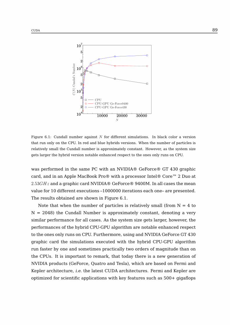
CUDA 89
104
2
5
105
2
5
106
2
5
107
10000 20000 30000
C(N
)Cundal’sNumber
N
CPUCPU-GPU Ge-Force9400CPU-GPU Ge-Force430
Figure 6.1: Cundall number against N for different simulations. In black color a version
that run only on the CPU. In red and blue hybrids versions. When the number of particles is
relatively small the Cundall number is approximately constant. However, as the system size
gets larger the hybrid version notable enhanced respect to the ones only runs on CPU.
was performed in the same PC with an NVIDIA® GeForce® GT 430 graphic
card, and in an Apple MacBook Pro® with a processor Intel® Core™ 2 Duo at
2.53GHz and a graphic card NVIDIA® GeForce® 9400M. In all cases the mean
value for 10 different executions –1000000 iterations each one– are presented.
The results obtained are shown in Figure 6.1.
Note that when the number of particles is relatively small (from N = 4 to
N = 2048) the Cundall Number is approximately constant, denoting a very
similar performance for all cases. As the system size gets larger, however, the
performances of the hybrid CPU-GPU algorithm are notable enhanced respect
to the ones only runs on CPU. Furthermore, using and NVIDIA GeForce GT 430
graphic card the simulations executed with the hybrid CPU-GPU algorithm
run faster by one and sometimes practically two orders of magnitude than on
the CPUs. It is important to remark, that today there is a new generation of
NVIDIA products (GeForce, Quatro and Tesla), which are based on Fermi and
Kepler architecture, i.e. the latest CUDA architectures. Fermi and Kepler are
optimized for scientific applications with key features such as 500+ gigaflops

90
of IEEE standard double precision floating point hardware support.
6.1.1 Realistic molecular dynamics implementation of spheres
on GPUs
The results of the benchmark confirm us that to develop an accurate hy-
brid MD-algorithm is a valid alternative to reduce the computing time in this
framework. Moreover, it leads us to a promising new prospect of real-time
simulations in dense granular media.
Starting from the CUDA particles example we have developed a realistic
molecular dynamics model for spheres with rotation. The first step was to
replace the Euler’s integrator by a Velocity Verlet integration method. This
modification notable improved the numerical output of the algorithm. First,
the global error of the Euler methods is of order one, whereas the global error
of the Velocity Verlet method is of order two. Additionally, this method guar-
anties that the total mechanical energy of the system always oscillates around
a constant value, which corresponds to the exactly solved system. The same
goes for others conservative quantities like linear or angular momentum, that
are always preserved or nearly preserved using this symplectic integrator.
On the other hand, the collision rules were changed to a generalized con-
tact law which is proved to be more realistic than the linear contact. Further-
more, new parameters for the energy dissipation due to collision were added.
The last upgrade, and the most important, was the incorporation of rotational
movement to the particles.
To define the normal interaction FNij , we use a nonlinear elastic force, de-
pending on the overlap distance δ of the particles. Moreover, to introduce
dissipation, a velocity dependent viscous damping is assumed. Hence, the to-
tal normal force reads as FNij = −kN · δα − γN · vNrel where kN is the spring
constant in the normal direction, γN is the damping coefficient in the normal
direction and vNrel is the normal relative velocity between i and j.
The tangential force F Tij also contains an elastic term and a tangential fric-
tional term accounting also for static friction between the grains. Taking into
account Coulomb’s friction law it reads as F Tij = min{−kT · ξ − γT · |vTrel|, µFN
ij }

CUDA 91
Figure 6.2: Six kinds of interactions between bonded particles: Pulling or pressing in ra-
dial direction (left, above), shearing in two tangential directions (middle and right, above),
twisting (left, bottom) and bending around two axes (middle and right, bottom).
where γT is the damping coefficient in tangential direction, vTrel is the tan-
gential component of the relative contact velocity of the overlapping pair. ξ
represents the elastic elongation of an imaginary spring with spring constant
kT at the contact [76], which increases as dξ(t)/dt = vTrel as long as there is an
overlap between the interacting particles [76, 183]. µ is the friction coefficient
of the particles.
Finally we solve the Newton’s equation of motion (1.5-3.1) for all particles
i (i = 1, ..., N)
6.1.2 Sphere Rotation on GPUs
Here, we focus our attention on the rotational part of the Newton’s equation
system
τ bi =N∑
j=1
Lij = Iiθi = Iiiωi (6.2)
ωi =τiIii
(i = 1, 2, 3) (6.3)

92
where ωi, τi and Iii are angular velocities, resultant torques and principal mo-
ment of inertia measured in the body-fixed frame.
There are different ways to represent orientation of a solid body, such as
Euler angles or quaternions representation. However, it has been demon-
strated that quaternions can offer fundamental computational, operational
and/or implementation and data handling advantages over conventional rota-
tional methods [214]. The unit quaternion q = (q0, q1, q2, q3) = q0+ q1i+ q2j+ q3k
is often used to describe the particle orientation [215, 216] where
i2 = j2 = k2 = ijk = −1ij = −ji = k
jk = −kj = i
ki = −ik = j
(6.4)
and3
∑
i=0
q2i = 1 (6.5)
The physical meaning of a quaternion is that it represents a one-step ro-
tation around the vector q1i + q2j + q3k with a rotation angle of 2 · arccos(q0)[214]. It is a very convenient tool due to some of its interesting features, such
as the fact that sequences of rotations can be conveniently represented as
quaternion product [214].
Quaternion for each particle satisfy the following equations of motion [215,
216]
q =1
2Q(q)ω (6.6)
where
q =
q0
q1
q2
q3
, Q(q) =
q0 −q1 −q2 −q3q1 q0 −q3 q2
q2 q3 q0 −q1q3 −q2 q1 q0
, ω =
0
ωx
ωy
ωz
.
Equations (6.3) and (6.6) govern the rotation of a particle and can be inte-
grated using Fincham’s leap-frog algorithm step by step [217], which is simple
and proved to be accurate enough. The approach obtains q(t + dt) from q(t)
CUDA 93
using
q(t+ dt) = q(t) + dt q(t) +dt2
2q(t) +O(dt3) = q(t) + dt q(t+ dt/2) +O(dt3) (6.7)
Hence, quaternion derivative at mid-step q(t + dt/2) is required. Equation
(6.6) indicates that q(t+ dt/2) and ω(t+ dt/2) are required, the former can be
easily calculated using
q(t+ dt/2) = q(t) + q(t)dt/2 (6.8)
where q(t) is again delivered by (6.6), prior to which ω(t) can be calculated
using
ω(t) = ω(t− dt/2) + I−1τ b(t)dt/2 (6.9)
and the later, ω(t+ dt/2), can be determined using
ω(t+ dt/2) = ω(t− dt/2) + I−1dt τ b(t) (6.10)
I is the inertia tensor expressed in the body-fixed frame. Hence, in this
algorithm, only ω(t−dt/2), q(t) need to be stored, the other quantities, such as
q(t+ dt/2), ω(t), q(t), q(t+ dt/2) are treated as temporary and auxiliary values.
To avoid the buildup errors, it is a common practice to renormalize quater-
nions at frequent intervals (usually done every step). The entire algorithm is
as follows
step 1: calculate torque τ(t) at time t.
step 2: using the stored ω(t− dt/2), update ω(t) using (6.9)
step 3: determine q(t) using (6.6)
step 4: using the stored ω(t− dt/2), calculate ω(t+ dt/2) using (6.10)
step 5: compute q(t+ dt/2) using (6.8)
step 6: evaluate q(t+ dt/2) using (6.6)
step 7: calculate q(t+ dt) using (6.7)
step 8: renormalize the quaternion q(t + dt).
6.2 Flowchart of the granular gas simulation
The application developed, as most of the GPGPU software, has an hetero-
geneous architecture. This means that some pieces of code run in the CPU

94
Figure 6.3: Flowchart of the granular gas simulation. Operations in gray run on the CPU,
subroutines in blue run on the GPU and the ones in oranges run partially in CPU and GPU.

CUDA 95
and others in the GPU. The flowchart of the discrete element method (DEM)
simulation program developed is presented in Figure 6.3. Procedures in gray
run in the CPU and the ones in blue in the GPU. The functions in orange are
executed partially in the CPU and partially in the GPU, and, in most cases,
they require data-interchange between CPU and GPU.
The first steps of the program consist in the initialization of the CUDA-
enable device, the allocation of the necessary memory –in both CPU and GPU–
and loading configuration parameters of the granular gas. Initially, the par-
ticles are homogeneously distributed in the simulation space with a random
velocity for translational and rotational movements (this is done on the host
and afterwards the particles’ information is sent to the device). With the objec-
tive of avoiding the initial configuration effect, the dissipation due to particle-
particle interaction is disable, and a number of free iterations is performed.
After that, the energy loss is enabled again and the main loop of the program
starts, calling in each iteration the Update System subroutine, and with a pe-
riodic frequency printing out the particles information. Finally the resources
reserved are released and the program ends.
The DEM process takes place in the Update System routine. Initially, fol-
lowing the Velocity Verlet integration method, the particles’ velocity in the
mid-point is calculated and with it the positions are updated. Then, with the
aim of minimizing the time used by the collisions method, the list with the par-
ticles that are neighbors to each other is updated. For details about the imple-
mentation of the neighbor function see the documentation given by NVIDIA
Corporation together with the CUDA particles example [212]. Next, the colli-
sions between particles are computed by calculation of the forces and torques
that a particle experiments. Finally, the last step of the Verlet integrator is per-
formed, obtaining the new velocities from the forces and using the algorithm
described in Section 6.1.2 to calculate angular velocities and positions.
6.3 Validation
The numerical accuracy of our model has been validated comparing it to the
mean field analytical solution of the homogeneous cooling of a gas of rough

96
and dissipative spherical particles. Luding et al [54] have found that transla-
tional and rotational kinetic energy of granular gas of rough and dissipative
particles in homogeneous cooling is governed by the following system of equa-
tions
ddτT = −AT 3/2 +BT 1/2RddτR = BT 3/2 − CT 1/2R
(6.11)
with the constants A, B and C, whose values depend on space dimensionality
D (for details see [54]).
A = 1−e2n4
+ η(1− η)
B = η2
q
C = ηq
(
1− ηq
)
(6.12)
where η = q(1 + et)/(2q + 2) (in 3D q = 2/5) and en and et are the restitution
coefficients on the normal and tangential direction respectively. Moreover,
the mean time between collisions G = 8(2a)2NV
√
πmg(2a), is used to rescale real
time scale accordingly to τ = 23GT
1/2tr (0)t. Moreover, the strength of the dissi-
pation can also be included into the characteristic time τ = 23(1− e2n)GT
1/2tr (0)t
[47].
To compare the numerical output of our code with the theoretical predic-
tions (Equations 6.11), we have to find equivalent dissipation parameters (γn,
γt and kt) that correspond to specific values of the normal en and tangential et
restitution coefficients.
6.3.1 Equivalent dissipative parameters
In the simplest approximation, the normal interaction force between two con-
tacting particles is a linear spring fnel = kNδ (α = 1 in Equation ??) and a
velocity dependent viscous damping fndiss = γnδ [70]. Examining the contact
evolution one gets the well known differential equation of the damped har-
monic oscillator [70]
δ + 2ηδ + w20δ = 0 (6.13)

CUDA 97
Here w0 =√
k/m12 is the oscillation frequency of an elastic oscillator and
η is the effective viscosity, obtained as
γn = 2 η m12 (6.14)
where m12 = m1m2/(m1 +m2) is the reduced mass. Solving Eq.(6.13) one can
find the effective restitution coefficient,
en = exp(−πη/ω) (6.15)
where
ω =√
ω20 − η2 (6.16)
is the oscillation frequency of the damped oscillator. Combining Equations
(6.15) and (6.16) and substituting in Equation (6.14) one obtains,
γn =
√
√
√
√
√
4 kn m12(
πln 1
en
)2
+ 1
(6.17)
On the other hand, describing the tangential force between to contacting
particles, one can also consider a tangential spring f tel = ktδ and a velocity
dependent viscous damping f tdiss = γtδ [70]. For the sake of simplicity, here we
examined the case γt = 0; for which an analytic expression, relating kt and kn,
can be derived,
kt =knq
1 + q
(
arccos(−et)π
)2
(6.18)
where q = 2/5 stands for the 3D case [70].
6.3.2 Numerical Results
We have numerically studied the free cooling kinetics of a dilute system of
N = 4096 spheres confined within a square box with l = 2, resulting a volume
fraction of Vf = 0.008. Initially, the particles are homogeneously distributed
in the space and their translational and rotational velocities follow a Gaussian
distribution. In order to avoid memory effects from the initial conditions, we
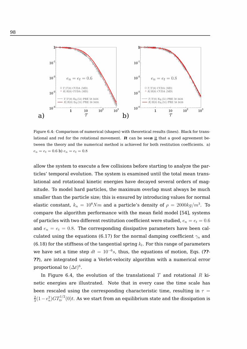
98
a)10
-4
10-3
10-2
10-1
11
11 10 102
103
T/T (0) Eq.(51) PRE 58 3416R/R(0) Eq.(51) PRE 58 3416
T/T (0) CUDA (MD)R/R(0) CUDA (MD)
en = et = 0.6
b)10
-4
10-3
10-2
10-1
11
11 10 102
103
T/T (0) Eq.(51) PRE 58 3416R/R(0) Eq.(51) PRE 58 3416
T/T (0) CUDA (MD)R/R(0) CUDA (MD)
en = et = 0.8
Figure 6.4: Comparison of numerical (shapes) with theoretical results (lines). Black for trans-
lational and red for the rotational movement. It can be seen it that a good agreement be-
tween the theory and the numerical method is achieved for both restitution coefficients. a)
en = et = 0.6 b) en = et = 0.8
allow the system to execute a few collisions before starting to analyze the par-
ticles’ temporal evolution. The system is examined until the total mean trans-
lational and rotational kinetic energies have decayed several orders of mag-
nitude. To model hard particles, the maximum overlap must always be much
smaller than the particle size; this is ensured by introducing values for normal
elastic constant, kn = 108Nm and a particle’s density of ρ = 2000kg/m3. To
compare the algorithm performance with the mean field model [54], systems
of particles with two different restitution coefficient were studied, en = et = 0.6
and en = et = 0.8. The corresponding dissipative parameters have been cal-
culated using the equations (6.17) for the normal damping coefficient γn and
(6.18) for the stiffness of the tangential spring kt. For this range of parameters
we have set a time step dt = 10−6s, thus, the equations of motion, Eqs. (??-
??), are integrated using a Verlet-velocity algorithm with a numerical error
proportional to (∆t)6.
In Figure 6.4, the evolution of the translational T and rotational R ki-
netic energies are illustrated. Note that in every case the time scale has
been rescaled using the corresponding characteristic time, resulting in τ =23(1− e2n)GT
1/2tr (0)t. As we start from an equilibrium state and the dissipation is

CUDA 99
0
20
40
60
80
100
120
0.0 0.01 0.02 0.03 0.04 0.05 0.06 0.07 0.08 0.09 0.1
D(v)
v
at t = 9× 10²
at t = 5× 10²
at t = 2× 10²
Maxwell-Boltzmann fit 1
Maxwell-Boltzmann fit 2
Maxwell-Boltzmann fit 3
Figure 6.5: Speed distribution for en = et = 0.8 at t = 2 × 10² (red), t = 5 × 10² (green) and
t = 9 × 10² (black). The velocity distributions follow Maxwell-Boltzmann statistics, indicating
that the system remains in the homogeneous cooling state.
0.0
0.05
0.1
0.15
0.2
0.25
0.3
0.35
0.4
-10 -5 0 5 10
D(ω
)
ω
ωx
ωy
ωz
Gaussian fit
t = 2× 10²
0.0
0.1
0.2
0.3
0.4
0.5
0.6
0.7
0.8
0.9
-4 -3 -2 -1 0 1 2 3 4
D(ω
)
ω
ωx
ωy
ωz
Gaussian fit
t = 5× 10²
0.0
0.2
0.4
0.6
0.8
1.0
1.2
1.4
-2.0 -1.5 -1.0 -0.5 0.0 0.5 1.0 1.5 2.0
D(ω
)
ω
ωx
ωy
ωz
Gaussian fit
t = 9× 10²
Figure 6.6: Angular velocity distribution for en = et = 0.8. left) at t = 2 × 10². center)
t = 5× 10². right) t = 9× 10². In all cases, the angular velocity distributions are in agreement
with a Gaussian behavior, denoting the homogeneous cooling process at the rotational level.

100
low, the system evolves into a homogeneous cooling state. In such a state, the
kinetic energy, decreases homogeneously and the time evolution of all vari-
ables occurs only through its global temperature. For comparison we also
show the corresponding analytic result of Eq. 6.11 for the same restitution
coefficients. The excellent agreement archived for both cases validates the
numerical performance of the new algorithm.
During the cooling process the velocity statistics was also examined. As we
mentioned earlier, the simulations begin from a Gaussian velocity distribution
for both, the translational and angular degree of freedom. Low dissipative par-
ticles cool down uniformly over a wide range of time. Thus, all the temporal
dependences enter through the mean values of the translational and rotational
temperature. Such a picture is consistent with the results shown in Fig. 6.5
(en = et = 0.8) where the speed distribution, D(c) and (c =√
v2x + v2y + v2z) is
presented at several times. In all cases, the speed distribution remains close to
a Maxwell-Boltzmann speed distribution D(c) = 4π(
1πv2mp
)3/2
c2e−c2/v2mp , where
vmp(t) is the most probable velocity. For the rotational degree of freedom, in
Fig. 6.6 we plot the angular velocity distribution for each angular component
obtained at different times. The data proves that cooling process at the ro-
tational level also occurs homogeneously. Thus, the three components of the
angular velocity behave equivalently and with the same characteristic values.
In all cases the distribution follows a Gaussian behavior f(wi) = 1σ√2πew
2i /2σ
2
featuring the expected homogeneous cooling process. The same procedure
was applied for en = et = 0.6 and similar results have been obtained (data not
show).
6.3.3 Optimal number of GPU
In any program that runs in parallel the execution time depends, in conjunc-
tion with the hardware, on the number of tasks running simultaneously. How-
ever, there is no an established way to define the optimal number of processors
to use within the hardware configuration. In programs that manipulate a big
volume of data this number depends, among other things, on the amount of
memory used per thread; the data interchanged between tasks may become a
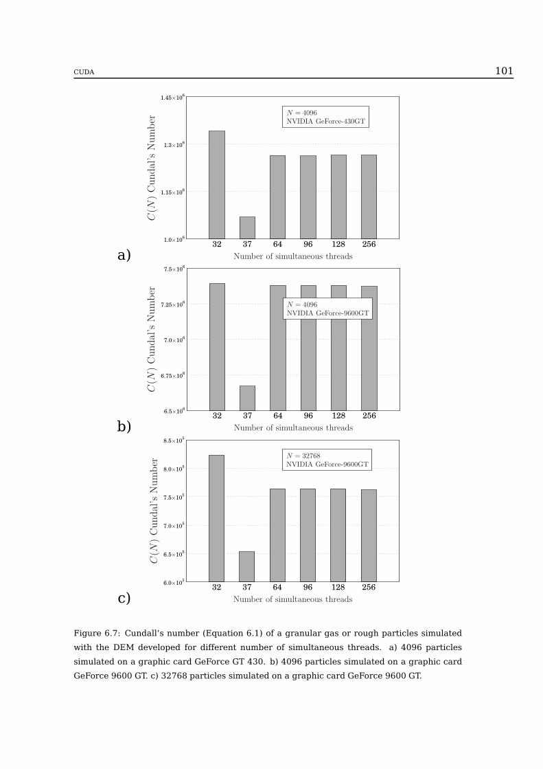
CUDA 101
a)1.0 10
6
1.15 106
1.3 106
1.45 106
32 37 64 96 128 256
C(N
)Cundal’sNumber
Number of simultaneous threads
N = 4096NVIDIA GeForce-430GT
b)6.5 10
6
6.75 106
7.0 106
7.25 106
7.5 106
32 37 64 96 128 256
C(N
)Cundal’sNumber
Number of simultaneous threads
N = 4096NVIDIA GeForce-9600GT
c)6.0 10
5
6.5 105
7.0 105
7.5 105
8.0 105
8.5 105
32 37 64 96 128 256
C(N
)Cundal’sNumber
Number of simultaneous threads
N = 32768NVIDIA GeForce-9600GT
Figure 6.7: Cundall’s number (Equation 6.1) of a granular gas or rough particles simulated
with the DEM developed for different number of simultaneous threads. a) 4096 particles
simulated on a graphic card GeForce GT 430. b) 4096 particles simulated on a graphic card
GeForce 9600 GT. c) 32768 particles simulated on a graphic card GeForce 9600 GT.

bottleneck.
To find the optimal value for the DEM created, a benchmark of a granu-
lar gas of rough particles was performed. The comparison was made in two
different NVIDIA graphic cards, in an NVIDIA® GeForce® GT 430 and in an
NVIDIA® GeForce® 9600 GT. In all cases the mean value for 10 different ex-
ecutions –1000000 iterations each one– are presented. In the first GPU the
simulation was of 4096 particles and in the second one the test was done for
4096 and 32768 particles. The result of the benchmark is shown in Figure 6.7.
For our hardware, 32 simultaneous threads seems to be the optimum value.
Furthermore, the results suggest that using a number that is not a power of
two –37 was used during the tests– is a bad decision. This can be inflicted by
taking a look to the architecture of the NVIDIA’s GPUs. The number of CUDA
Cores present in all their graphics cards is a power of two. Therefore, using
a value that is not power of two result in wasting part of the processor each
time.
6.4 Conclusions
In typical technological process the flows contain billions of particles and the
main disadvantages of molecular dynamics algorithms implemented on com-
puting processing units (CPU) are the maximum number of particles and the
duration of a virtual simulation. In this chapter we have described the im-
plementation of an accurate molecular dynamic algorithm for mono-disperse
systems of spheres with rotation, using graphical processing units (GPUs).
The employment of this technique saves a huge computational time versus
the traditional CPU method. Moreover, we have proved that the algorithm
complies with the statistical mechanical laws and the results agree with es-
tablished mean field theories for low dense granular systems. Our results are
in excellent agreement with a previous mean field analytical model, which de-
scribes the cooling dynamics of a system composed by dissipative and rough
spheres. All this leads us to a promising new prospect of real-time simulations
in many different technological scenarios concerning dense granular media.

Chapter 7
General conclusions
A novel numerical scheme to simulate the kinetics of non-linear frag-
mentation equations have been introduced. The method is based on the
Direct Simulation Monte Carlo (DSMC) technique for solving the Boltzmann
equation. This approach have been generalized for solving kinetic equations
where the number of particles vary changes in time. Hence, we have vali-
dated the algorithm examining simplest fragmentation kernels, where exact
solutions exist. The proposed approach recover the detailed time evolution
accurately, as well as the emergence of asymptotic scaling regimes. Such a
comparison has shown the ability of the scheme to cover a significant number
of decades in order to capture the broad size distributions characterizing frag-
menting systems, thus making it possible to carry out quantitative, detailed
comparisons. We have extended and made use of the algorithm to analyze
general fragmentation kernels, where exact analytic predictions for the kinet-
ics of fragmenting systems are lacking. Furthermore, we have shown that
with the good statistics achieved with the numerical technique proposed, it is
possible to follow the development of an advancing front for generic asymmet-
ric fragmentation kernels. Such an understanding promotes confidence in the
development of scaling distribution functions.
The cooling dynamics of a 2D granular gas of elongated grains have
been examined. For weakly dissipative particles, we have found that the
mean kinetic energy decreases asymptotically as E(t)E0
= 1(1+t/to)5/3
, in agreement
with Brilliantov and Pöschel predictions for the homogeneous cooling state
103

104
regimen (HCS) of viscoelastic particles [46, 158]. A higher dissipation induces
an inhomogeneous cooling process and the energy vanishes as E(t)E0∼ t−1.2. The
rotational energy, however, always decays as R(t)R0∼ t−2, which is agreement
with Haff’s prediction for the HCS of inelastic particles. The lack of energy
equipartition is kept even during the inhomogeneous cooling process where
strong inhomogeneities in the velocity field are presented. A strong influence
of the particle shape and inelasticity on the structure of the clusters have
been observed. Our numerical outcomes suggest that the strong dissipation
and the particle anisotropy induce the formation of ordered cluster structures
and velocity vortices, which notably slow down the cooling process and retard
the appearance of large clusters which break and reform. Increasing the par-
ticle anisotropy enhances this distinct evolution as a function of the particle
energy dissipation. This behavior can be attributed to the detailed interaction
between ordered clusters of particles, where rotational degrees of freedom
play a relevant role. The breakup of big clusters of elongated particles as a
results of their collisions leads to the formation of smaller clusters, promoting
a faster decay of the rotational kinetic energy. Such smaller clusters of or-
dered particles in turn delay the development of the inhomogeneous cooling
regime. Understanding the impact of these strong correlations in agitated sys-
tems where energy is supplied continuously constitutes an interesting venue
in the fundamental understanding of the physics of anisotropic granulates and
the subtle interplays between particle shape and inelasticity.
The micro-mechanical properties of deposits of faceted particles
have been examined, in details. For instance, the partial discharge of a
silo filled with faceted grains has a profound effect on the deposit morphology
and its stress distribution. During the discharge, the shear between grains
induces their rotation and their settlement in more disordered arrangements.
For elongated particles, the preferred horizontal orientation displayed after
the silo filling disappears. For square particles, the discharge provokes an
alignment of their sides with gravity which minimizes the friction and favors
their vertical displacement. As a result of the changes in particle orientation,
the pressure distribution in the silo changes qualitatively; while for elongated
rods lateral stress transmission is promoted by the enhanced disorder leading

General conclusions 105
to a faster pressure saturation, the opposite holds for squares. In this latter
case the alignment of squares induced by the flow destroys the initial force
chain network which is replaced by a mainly vertical stress transmission. As
a consequence, a significant reduction of the pressure saturation effect is ob-
served. With this results, we clarified the performance and stability of silos,
which need to support high stresses that become very sensitive to grain shapes
and the silo steering history. If we increase the amount of material flowing out
of the silo, or induce a second discharge, we expect that the observed effect
will be enhanced. Although we have focused on weakly disordered initial de-
posits, due to the low feeding rates used to fill the silo, the main features dis-
cussed here are expected for other silo filling procedures. Perhaps, increasing
the disorder of the initial packing will generically decrease the relative mag-
nitude of the changes discussed.
To introduce an attractive force in deposits of elongated grains has
a profound effect on the deposit morphology and its stress profiles.
In deposits of non-cohesive particles the topology is dominated by the forma-
tion of ordered structures of aligned rods. Elongated particles tend to align
horizontally and the stress is mainly transmitted from top to bottom, reveal-
ing an asymmetric distribution of the local stress. Lateral force transmission
becomes less favored compared to vertical transfer, thus hindering pressure
saturation with depth. For deposits of cohesive particles, the preferred hori-
zontal orientation is less pronounced with increasing cohesion. Very elongated
particles with strong attractive forces form extremely loose structures, char-
acterized by orientation distributions, which tend to a uniform behavior when
increasing the Bond number. As a result of these changes, the pressure distri-
bution in the deposits changes qualitatively. The spherical component of the
local stress is notably enhanced with respect to the deviatoric part. Hence,
the lateral stress transmission is promoted by the enhanced disorder and it
leads to a faster pressure saturation with depth.
The implementation of an accurate molecular dynamic algorithm
for mono-disperse systems of spheres with rotation, using graphical
processing units (GPUs) was described in details. The employment of
this technique saves a huge computational time versus the traditional CPU

method. Moreover, we have proved that the algorithm complies with the sta-
tistical mechanical laws and the results agree with established mean field the-
ories for low dense granular systems. Our results are in excellent agreement
with a previous mean field analytical model, which describes the cooling dy-
namics of a system composed by dissipative and rough spheres. All this leads
us to a promising new prospect of real-time simulations in many different tech-
nological scenarios concerning dense granular media.
Bibliography
[1] J. Duran, Sands, Powders, and Grains: An Introduction to the Physics of
Granular Materials. Springer, 1 ed., 1999.
[2] G. E. Moore, “Cramming more components onto integrated circuits,”
Electronics, vol. 38, p. 114, April 1965.
[3] G. E. Moore, “Progress in digital integrated electronics,” in Electron
Devices Meeting, 1975 International, vol. 21, pp. 11–13, 1975.
[4] N. Metropolis and S. Ulam, “The monte carlo method,” Journal of the
American Statistical Association, vol. 44, p. 247, 1949.
[5] B. Alder and T. Wainwright, “Phase transition for a hard sphere system,”
J. Chem. Phys., vol. 24, no. 5, p. 1208, 1957.
[6] B. Alder and T. Wainwright, “Studies in molecular dynamics. i. general
method,” J. Chem. Phys., vol. 31, no. 2, p. 459, 1959.
[7] N. Metropolis, “The beginning of the monte carlo method,” Los Alamos
Science, Special Issue, vol. 15, pp. 125–130, 1987.
[8] J. Hammersley, “Monte carlo methods for solving multivariable prob-
lems,” Annals of the New York Academy of Sciences, vol. 86, no. 3,
pp. 844–874, 1960.
[9] W. Press, B. Flannery, S. Teukolsky, and W. Vetterling, Numerical
Recipes in FORTRAN: The Art of Scientific Computing., ch. 7.6 Sim-
ple Monte Carlo Integration, pp. 295–299. Cambridge University Press,
2nd ed., 1992.
107

108
[10] W. Press, B. Flannery, S. Teukolsky, and W. Vetterling, Numerical
Recipes in FORTRAN: The Art of Scientific Computing., ch. 7.8 Adaptive
and Recursive Monte Carlo Methods, pp. 306–319. Cambridge Univer-
sity Press, 2nd ed., 1992.
[11] K. Binder, ed., The Monte Carlo Method in Condensed Matter Physics.
New York: Springer, 2nd ed., December 1995.
[12] P. Mackeown, Stochastic Simulation in Physics. Secaucus, NJ, USA:
Springer Verlag, Singapore, 2001.
[13] W. C. H. Gould, J. Tobochnik, An Introduction to Computer Simulation
Methods: Applications to Physical Systems. Pearson Addison Wesley,
3rd ed., 2007.
[14] D. Landau and K. Binder, A Guide to Monte Carlo Simulations in Statis-
tical Physics. Cambridge University Press, 3 ed., October 2009.
[15] I. Pagonabarraga, T. Kanzaki, and R. Hidalgo, “Collision induced frag-
mentation: A simplenumerical algorithm,” Eur. Phys. J. Special Topics,
vol. 179, pp. 43–53, 2009.
[16] K. Binder and D. Heermann, Monte Carlo Simulation in Statistical
Physics: An Introduction. New York: Springer, 5th ed., August 2010.
[17] J. Farjas and P. Roura, “Numerical model of solid phase transformations
governed by nucleation and growth: Microstructure development dur-
ing isothermal crystallization,” Phys. Rev. B, vol. 75, no. 18, p. 184112,
2007.
[18] F. Dellaert, D. Fox, W. Burgard, and S. Thrun, “Monte carlo localization
for mobile robots,” in IEEE International Conference on Robotics and
Automation (ICRA99), pp. 1322–1328, May 1999.
[19] S. Thrun., D. Fox, W. Burgard, and F. Dellaert, “Robust monte carlo
localization for mobile robots,” Artificial Intelligence, vol. 128, no. 1-2,
pp. 99–141, 2001.

Bibliography 109
[20] T. Li, S. Sun, and J. Duan, “Monte carlo localization for mobile robot us-
ing adaptive particle merging and splitting technique,” in Proceedings
of the 2010 IEEE International Conference on Information and Automa-
tion, (Harbin), pp. 1913–1918, June 2010.
[21] G. Drusano, D. D’Argenio, S. Preston, C. Barone, W. Symonds, S. LaFon,
M. Rogers, W. Prince, A. Bye, and J. A. Bilello, “Use of drug effect in-
teraction modeling with monte carlo simulation to examine the impact
of dosing interval on the projected antiviral activity of the combination
of abacavir and amprenavir,” Antimicrobial Agents and Chemotherapy,
vol. 44, no. 6, pp. 1655–1659, 2000.
[22] H. Paganetti, “Monte carlo calculations for absolute dosimetry to de-
termine machine outputs for proton therapy fields,” Phys. Med. Biol.,
vol. 51, no. 11, p. 2801, 2006.
[23] S. Kim, “Characteristics of elliptical sources in beamnrc monte carlo
system: Implementation and application,” Med. Phys., vol. 36, no. 4,
p. 1046, 2009.
[24] D. Merl, L. Johnson, R. Gramacy, and M. Mangel, “A statistical frame-
work for the adaptive management of epidemiological interventions,”
PLoS ONE, vol. 4, no. 6, p. e5807, 2009.
[25] C. Forastero, L. Zamora, D. Guirado, and A. Lallena, “A monte carlo tool
to simulate breast cancer screening programmes,” Physics in Medicine
and Biology, vol. 55, no. 17, p. 5213, 2010.
[26] C. Mode, ed., Applications of Monte Carlo Methods in Biology, Medicine
and Other Fields of Science. Rijeka, Croatia: InTech, February 2011.
[27] P. Boyle, M. Broadie, and P. Glasserman, “Monte carlo methods for
security pricing,” Journal of Economic Dynamics and Control, vol. 21,
pp. 1267–1321, June 1997.
[28] D. Vose, Risk analysis: a quantitative guide. John Wiley & Sons, 2nd ed.,
2000.

110
[29] J. Charnes and P. Shenoy, “Multistage monte carlo method for solv-
ing influence diagrams using local computation,”Management Science,
vol. 50, pp. 405–418, March 2004.
[30] C. Beveridge and M. Joshi, “Monte carlo bounds for game options in-
cluding convertible bonds,”Management Science, vol. 57, pp. 960–974,
April 2011.
[31] C. Grinstead and J. Snell, Introduction to Probability, ch. 9. Central Limit
Theorem, pp. 325–360. American Mathematical Soc., 2nd ed., 1997.
[32] G. Fishman, Monte Carlo: concepts, algorithms, and applications.
Springer series in operations research, New York, USA: New York:
Springer, 1996.
[33] N. Metropolis, A. Rosenbluth, M. Rosenbluth, A. Teller, and E. Teller,
“Equation of state calculations by fast computing machines,” J. Chem.
Phys, vol. 21, p. 1087, 1953.
[34] W. Hastings, “Monte carlo sampling methods using markov chains and
their applications,” Boimetrika, vol. 57, pp. 97–109, July 1970.
[35] G. Birkhoff, “Proof of the ergodic theorem,” Proc Natl Acad Sci USA,
vol. 17, no. 12, pp. 656‚Äì–660, 1931.
[36] J. von Neumann, “Physical applications of the ergodic hypothesis,” Pro-
ceedings of the National Academy of Sciences of the United States of
America, vol. 18, no. 3, pp. 263–266, 1932.
[37] G. Birkhoff, “What is the ergodic theorem?,” Mathematical Association
of America, vol. 49, no. 4, pp. 222–226, 1942.
[38] P. Walters, An Introduction to Ergodic Theory (Graduate Texts in Math-
ematics). Springer, October 2000.
[39] G. Bird, “Approach to translational equilibrium in a rigid sphere gas,”
Phys. Fluids, vol. 6, p. 1518, 1963.
Bibliography 111
[40] A. Rahman, “Correlations in the motion of atoms in liquid argon,” Phys.
Rev., vol. 136, no. 2A, pp. A405‚Äì–A411, 1964.
[41] L. Verlet, “Computer "experiments" on classical fluids. i. thermodynam-
ical properties of lennard-jones molecules,” Phys. Rev., vol. 159, no. 1,
pp. 98–103, 1967.
[42] L. Verlet, “Computer "experiments" on classical fluids. ii. equilibrium
correlation functions,” Phys. Rev., vol. 165, no. 1, pp. 201–214, 1968.
[43] T. Pöschel and T. Schwager, Computational Granular Dynamics.
Springer-Verlag Berlin Heidelberg New York, 2005.
[44] M. Allen and D. Tildesley, Computer Simulation of Liquids. Clarendon
Press, Oxford, 1987.
[45] I. Goldhirsch and G. Zanetti, “Clustering instability in dissipative
gases,” Phys. Rev. Lett., vol. 70, no. 11, pp. 1619–1622, 1993.
[46] N. Brilliantov and T. Pöschel, “Velocity distribution in granular gases of
viscoelastic particles,” Phys. Rev. E, vol. 61, p. 5573, 2000.
[47] S. Miller and S. Luding, “Cluster growth in two- and three-dimensional
granular gases,” Phys. Rev. E, vol. 69, p. 031305, 2004.
[48] S. Miller and S. Luding, “Event-driven molecular dynamics in parallel,”
Journal of Computational Physics, vol. 193, no. 1, pp. 306–316, 2004.
[49] J. Jenkins and M. Richman, “Kinetic theory for plane flows of a dense gas
of identical, rough, inelastic, circular disks,” Physics of Fluids, vol. 28,
no. 12, p. 3485, 1985.
[50] M. Huthmann and A. Zippelius, “Dynamics of inelastically colliding
rough spheres: Relaxation of translational and rotational energy,” Phys.
Rev. E, vol. 56, pp. R6275–R6278, 1997.
[51] S. McNamara and S. Luding, “Energy nonequipartition in systems of
inelastic, rough spheres,” Phys. Rev. E, vol. 58, no. 2, pp. 2247‚Äì–2250,
1998.
112
[52] R. Cafiero, S. Luding, and H. Herrmann, “Rotationally driven gas of
inelastic rough spheres,” EPL (Europhysics Letters), vol. 60, p. 854,
2002.
[53] E. Ben-Naim, S. Chen, G. Doolen, and S. Redner, “Shocklike dynamics
of inelastic gases,” Phys. Rev. Lett., vol. 83, p. 4069, 1999.
[54] S. Luding, M. Huthmann, S. McNamara, and A. Zippelius, “Homoge-
neous cooling of rough dissipative particles: Theory and simulations,”
Phys. Rev. E, vol. 58, pp. 3416–3425, 1998.
[55] R. Cafiero, S. Luding, and H. Herrmann, “Two-dimensional granular gas
of inelastic spheres with multiplicative driving,” Phys. Rev. Lett., vol. 84,
pp. 6014–6017, 2000.
[56] T. Aspelmeier, G. Giese, and A. Zippelius, “Cooling dynamics of a dilute
gas of inelastic rods: A many particle simulation,” Phys. Rev. E, vol. 57,
p. 857, 1998.
[57] A.Donev, S. Torquato, and F. Stillinger, “Neighbor list collision-driven
molecular dynamics simulation for nonspherical hard particles. i. al-
gorithmic details,” Journal of Computational Physics, vol. 202, no. 2,
pp. 737–764, 2005.
[58] A.Donev, S. Torquato, and F. Stillinger, “Neighbor list collision-driven
molecular dynamics simulation for nonspherical hard particles.: Ii. ap-
plications to ellipses and ellipsoids,” Journal of Computational Physics,
vol. 202, no. 2, pp. 765–793, 2005.
[59] M. Bannerman and L. Lue, “Transport properties of highly asymmetric
hard-sphere mixtures,” Journal of Chemical Physics, vol. 130, no. 16,
p. 164507, 2009.
[60] S. González, A. Thornton, and S. Luding, “An event-driven algorithm for
fractal cluster formation,” Computer Physics Communications, vol. 182,
no. 9, pp. 1842–1845, 2011.

Bibliography 113
[61] Y. Taguchi, “Powder turbulence: direct onset of turbulent flow,” J. Phys.
II France, vol. 2, no. 12, pp. 2103–2114, 1992.
[62] R. Ramírez, T. Pöschel, N. Brilliantov, and T. Schwager, “Coefficient of
restitution of colliding viscoelastic spheres,” Phys. Rev. E, vol. 60, no. 4,
pp. 4465–4472, 1999.
[63] F. Bridges, A. Hatzes, and D. Lin, “Structure, stability and evolution of
saturn’s rings,” Nature, vol. 309, pp. 333–335, 1984.
[64] S. Luding, E. Clément, A. Blumen, J. Rajchenbach, and J. Duran, “Anoma-
lous energy dissipation in molecular dynamics simulations of grains:
The "detachment effect”,” Phys. Rev. E, vol. 50, p. 4113, 1994.
[65] S. Foerster, M. Louge, H. Chang, and K. Allia, “Measurements of the
collision properties of small spheres,” Physics of Fluids, vol. 6, no. 3,
p. 1108, 1993.
[66] E. Falcon, C. Laroche, S. Fauve, and C. Coste, “Behavior of one inelastic
ball bouncing repeatedly off the ground,” The European Physical Jour-
nal B, vol. 3, no. 1, pp. 45–57, 1998.
[67] F. Gerl and A. Zippelius, “Coefficient of restitution for elastic disks,”
Phys. Rev. E, vol. 59, no. 2, pp. 2361‚Äì–2372, 1999.
[68] T. Schwager, “Coefficient of restitution for viscoelastic disks,” Phys. Rev.
E, vol. 75, p. 051305, 2007.
[69] P. Müller and T. Pöschel, “Collision of viscoelastic spheres: Compact ex-
pressions for the coefficient of normal restitution,” Phys. Rev. E, vol. 84,
no. 2, p. 021302, 2011.
[70] S. Luding, “Collisions & contacts between two particles,” in Physics
of dry granular media - NATO ASI Series E350 (H. J. Herrmann, J.-P.
Hovi, and S. Luding, eds.), (Dordrecht), pp. 285–304, Kluwer Academic
Publishers, 1998.
[71] F. Kun and H. Herrmann, “Transition from damage to fragmentation in
collision of solids,” Phys. Rev. E, vol. 59, pp. 2623–2632, 1999.

114
[72] F. Alonso-Marroquín, I. Vardoulakis, H. Herrmann, D. Weatherley, and
P. Mora, “Effect of rolling on dissipation in fault gouges,” Phys. Rev. E,
vol. 74, p. 031306, 2006.
[73] A. Pena, P. Lind, and H. Herrmann, “Modeling slow deformation of
polygonal particles using dem,” Particuology, vol. 6, no. 6, pp. 506–514,
2008.
[74] H.-J. Tillemans and H. Herrmann, “Simulating deformations of granular
solids under shear,” Physica A, vol. 217, pp. 261–288, 1995.
[75] F. Kun and H. Herrmann, “A study of fragmentation processes using
a discrete element method,” Computer Methods in Applied Mechanics
and Engineering, vol. 138, pp. 3–18, 1996.
[76] P. Cundall and O. Strack, “A discrete numerical model for granular as-
semblies,” Geotechnique, vol. 29, pp. 47–‚Äì65, 1979.
[77] A. Pena, P. Lind, S. McNamara, and H. Herrmann, “Numerical improve-
ment of the discrete element method applied to shear of granular me-
dia.” Condensed matter, 2007.
[78] A. Pena, R. García-Rojo, and H. Herrmann, “Influence of particle shape
on sheared dense granular media,” Granular Matter, vol. 9, pp. 279–
291, 2007.
[79] A. Iserles, A first course in the numerical analysis of differential equa-
tions. Cambridge texts in applied mathematics. Issue 15 of Texts in Ap-
plied Mathematics, Cambridge, England: Cambridge University Press,
1996.
[80] M. Alvarez, A. Guerra, and R. Lau, Matemática Numérica. La Habana,
Cuba: Editorial Félix Varela, 2nd ed., 2004.
[81] J. Lambert, Numerical methods for ordinary differential systems: the
initial value problem. New York, NY, USA: John Wiley & Sons, 1991.
[82] J. Butcher, Numerical methods for ordinary differential equations. New
York, NY, USA: John Wiley and Sons, 2nd ed., 2008.

Bibliography 115
[83] K. New, K. Watt, C. Misner, and J. Centrella, “Stable 3-level leapfrog in-
tegration in numerical relativity,” Phys. Rev. D, vol. 58, no. 6, p. 064022,
1998.
[84] E. Hairer, C. Lubich, and G. Wanner, “Geometric numerical integra-
tion illustrated by the störmer-verlet methods,” Acta Numerica, vol. 12,
pp. 399–450, 2003.
[85] G. Forsythe, M. Malcolm, and C. Moler, Computer methods for mathe-
matical computations. Prentice-Hall, 1977.
[86] E. Hairer, S. Nørsett, and G. Wanner, Solving ordinary differential equa-
tions: Nonstiff problems, vol. Volume 1 of Solving Ordinary Differential
Equations, Gerhard Wanner of Springer series in computational mathe-
matics. Springer, 2nd ed., 1993.
[87] C. Gear, Numerical Initial Value Problems in Ordinary Differential Equa-
tions. NJ, USA: Prentice Hall, 1st ed., September 1971.
[88] W. Press, S. Teukolsky, W. Vetterling, and B. Flannery, Numerical
Recipes 3rd Edition: The Art of Scientific Computing, ch. 17.6. Multi-
step, Multivalue, and Predictor-Corrector Methods, pp. 942–946. Cam-
bridge University Press, 3rd ed., September 2007.
[89] K. Schoen, “Fifth and sixth order pece algorithms with improved sta-
bility properties,” SIAM Journal on Numerical Analysis, vol. 8, no. 2,
pp. 244–248, 1971.
[90] M. Greenberg, Advanced engineering mathematics. Michigan, USA:
Prentice Hall, November 1988.
[91] W. Press, S. Teukolsky, W. Vetterling, and B. Flannery, Numerical
Recipes 3rd Edition: The Art of Scientific Computing. Cambridge Uni-
versity Press, 3rd ed., 2007.
[92] W. Swope, H. Andersen, P. Berens, and K. Wilson, “A computer simu-
lation method for the calculation of equilibrium constants for the for-
116
mation of physical clusters of molecules: Application to small water
clusters,” J. Chem. Phys., vol. 76, no. 1, pp. 637–649, 1982.
[93] R. Arévalo, Dinámica microscópica en la descarga de silos y redes
de fuerza en un medio granular rígido. PhD thesis, Universidad de
Navarra, 2009.
[94] T. Sterling, “An introduction to pc clusters for high performance com-
puting,” International Journal of High Performance Computing Applica-
tions, vol. 15, pp. 92–101, May 2001.
[95] D. Bader and R. Pennington, “Cluster computing: Applications,” Inter-
national Journal of High Performance Computing Applications, vol. 15,
pp. 181–185, May 2001.
[96] T. Rauber and G. Rünger, Parallel Programming: for Multicore and Clus-
ter Systems. Springer, 2010.
[97] J. Owens, D. Luebke, N. Govindaraju, M. Harris, J. Krüger, A. Lefohn, and
T. Purcell, “A survey of general-purpose computation on graphics hard-
ware,” Computer Graphics Forum, vol. 26, pp. 80–113, March 2007.
[98] J. Owens, M. Houston, D. Luebke, S. Green, J. Stone, and J. Phillips,
“Gpu computing,” Proceedings of the IEEE, vol. 96, pp. 879–899, May
2008.
[99] J. Sanders and E. Kandrot, CUDA by Example: An Introduction to
General-Purpose GPU Programming. Addison-Wesley Professional,
2010.
[100] A. Grama, G. Karypis, V. Kumar, and A. Gupta, Introduction to Parallel
Computing. Addison Wesley, 2nd ed., 2003.
[101] J. England, “A system for interactive modeling of physical curved sur-
face objects,” SIGGRAPH Comput. Graph., vol. 12, pp. 336–340, August
1978.
[102] M. Potmesil and E. Hoffert, “The pixel machine: a parallel image com-
puter,” SIGGRAPH Comput. Graph., vol. 23, pp. 69–78, July 1989.

Bibliography 117
[103] J. Lengyel, M. Reichert, B. Donald, and D. Greenberg, “Real-time robot
motion planning using rasterizing computer graphics hardware,” SIG-
GRAPH Comput. Graph., vol. 24, pp. 327–335, September 1990.
[104] J. Rhoades, G. Turk, A. Bell, A. State, U. Neumann, and A. Varshney,
“Real-time procedural textures,” in Proceedings of the 1992 symposium
on Interactive 3D graphics, I3D ’92, (New York, NY, USA), pp. 95–100,
ACM, 1992.
[105] C. Trendall and A. Stewart, “General calculations using graphics hard-
ware with applications to interactive caustics,” in Proceedings of the
Eurographics Workshop on Rendering Techniques 2000, (London, UK),
pp. 287–298, Springer-Verlag, 2000.
[106] M. Harris, G. Coombe, T. Scheuermann, and A. Lastra, “Physically-
based visual simulation on graphics hardware,” in Proceedings of the
ACM SIGGRAPH/EUROGRAPHICS conference on Graphics hardware,
HWWS ’02, (Aire-la-Ville, Switzerland, Switzerland), pp. 109–118, Euro-
graphics Association, 2002.
[107] E. Lindholm, M. Kilgard, and H. Moreton, “A user-programmable vertex
engine,” in Proceedings of the 28th annual conference on Computer
graphics and interactive techniques, SIGGRAPH ’01, (New York, NY,
USA), pp. 149–158, ACM, 2001.
[108] NVIDIA, “Nvidia developer zone web page.”
http://developer.nvidia.com/category/zone/cuda-zone, Septem-
ber 2011.
[109] AMD, “Amd accelerated parallel processing sdk.”
http://developer.amd.com/sdks/AMDAPPSDK/Pages/default.aspx,
September 2011.
[110] Khronos, “Opencl - the open standard for parallel programming of het-
erogeneous systems.” http://www.khronos.org/opencl/, September
2011.

118
[111] NVIDIA,NVIDIA CUDA C Programming Guide. NVIDIA Developer Zone,
2011.
[112] NVIDIA, “Cuda gpus at nvidia developer zone.”
http://developer.nvidia.com/cuda-gpus, September 2011.
[113] NVIDIA, “Nvidia gpu computing sdk web site.”
http://developer.nvidia.com/gpu-computing-sdk, September
2011.
[114] C. Chang, Y. Chang, M. Huang, and B. Huang, “Accelerating regular
ldpc code decoders on gpus,” IEEE Journal of Selected Topics in Applied
Earth Observations and Remote Sensing, vol. 4, no. 3, pp. 653–659,
2011.
[115] J. Mielikainen, H. Bormin, and H. Huang, “Gpu-accelerated multi-profile
radiative transfer model for the infrared atmospheric sounding interfer-
ometer,” IEEE Journal of Selected Topics in Applied Earth Observations
and Remote Sensing, vol. 4, no. 3, pp. 691–700, 2011.
[116] E. Christophe, L. Michel, and J. Inglada, “Remote sensing processing:
From multicore to gpu,” IEEE Journal of Selected Topics in Applied
Earth Observations and Remote Sensing, vol. 4, no. 3, pp. 643–652,
2011.
[117] S. Changhe, L. Yunsong, and H. Bormin, “A gpu-accelerated wavelet de-
compression system with spiht and reed-solomon decoding for satellite
images,” IEEE Journal of Selected Topics in Applied Earth Observations
and Remote Sensing, vol. 4, no. 3, pp. 683–690, 2011.
[118] J. Cui, G. Pratx, S. Prevrhal, and C. Levin, “Fully 3d list-mode time-of-
flight pet image reconstruction on gpus using cuda,”Med. Phys., vol. 38,
no. 12, pp. 6775–6786, 2011.
[119] E. van Aart, N. S, A. Jalba, and A. Vilanova, “Cuda-accelerated geodesic
ray-tracing for fiber tracking,” International Journal of Biomedical
Imaging, vol. 2011, p. 698908, 2011.
Bibliography 119
[120] S. Park, B. Kim, L. Lee, J. Goo, and Y. Shin, “Ggo nodule volume-
preserving nonrigid lung registration using glcm texture analysis,”
IEEE Trans Biomed Eng., vol. 58, no. 10, pp. 2885–2894, 2011.
[121] Z. Grof, J. Kosek, M. Marek, and P. Adler, “Modeling of morphogenesis
of polyolefin particles: Catalyst fragmentation,” AIChE, vol. 49, no. 4,
pp. 1002–1013, 2003.
[122] L. Oddershede, P. Dimon, and J. Bohr, “Self-organized criticality in frag-
menting,” Phys. Rev. Lett., vol. 71, no. 19, pp. 3107–3110, 1993.
[123] F. Wittel, F. Kun, H. Herrmann, and B. Kröplin, “Fragmentation of
shells,” Phys. Rev. Lett., vol. 93, no. 3, p. 035504, 2004.
[124] F. Kun, F. Wittel, H. Herrmann, B. K. K.J., and Måløy, “Scaling behavior
of fragment shapes,” Phys. Rev. Lett., vol. 96, no. 2, p. 025504, 2006.
[125] D. Nesvorny, D. Vokrouhlicky, W. Bottke, and M. Sykes, “Physical proper-
ties of asteroid dust bands and their sources,” ICARUS, vol. 181, no. 1,
pp. 107–144, 2006.
[126] A. Weber, U. Teipel, and H. Nirschl, “Comparison of comminution by
impact of particle collectives and other grinding processes,” Chem. Eng.
& Tech., vol. 29, no. 5, pp. 642–648, 2006.
[127] O. Sotolongo-Costa, Y. Moreno-Vega, J. Lloveras-González, and J. An-
toranz, “Criticality in droplet fragmentation,” Phys. Rev. Lett., vol. 76,
no. 1, pp. 42–45, 1996.
[128] T. Jiang and J. Northby, “Fragmentation clusters formed in supercritical
expansions of 4He,” Phys. Rev. Lett., vol. 68, no. 17, pp. 2620–2623,
1992.
[129] S. Redner, Statistical Models for the Fracture of Disordered Media,
ch. Fragmentation. Amsterdam: Elsevier Science Pubs, North-Holland,
1990.
[130] E. McGrady and R. Ziff, “”shattering” transition in fragmentation,”
Phys. Rev. Lett., vol. 58, no. 9, pp. 892–895, 1987.

120
[131] Z. Cheng and S. Redner, “Kinetics of fragmentation,” J. Phys. A, vol. 23,
no. 7, p. 1233, 1990.
[132] M. Ernst and G. Szamel, “Fragmentation kinetics,” J. Phys. A, vol. 26,
no. 22, p. 6085, 1993.
[133] P. Krapivsky and E. Ben-Naim, “Shattering transitions in collision-
induced fragmentation,” Phys. Rev. E, vol. 68, no. 2, p. 021102, 2003.
[134] M. Ernst and I. Pagonabarraga, “The nonlinear fragmentation equa-
tion,” J. Phys. A, vol. 40, no. 17, p. F331, 2007.
[135] J. Aström, “Statistical models of brittle fragmentation,” Adv. Phys.,
vol. 55, no. 3–4, pp. 247–278, 2006.
[136] F. Spahn, N. Albers, M. Sremcevic, and C. Thornton, “Kinetic descrip-
tion of coagulation and fragmentation in dilute granular particle ensem-
bles,” Europhys. Lett., vol. 67, no. 4, p. 545, 2004.
[137] I. Pagonabarraga and E. Trizac, Granular Gas Dynamics, vol. 624, ch. Ki-
netics of Fragmenting Freely Evolving Granular Gases, pp. 163–184.
Berlin: Springer-Verlag, 2003.
[138] R. Hidalgo and I. Pagonabarraga, “Fragmenting granular gases,” Euro-
phys. Lett., vol. 77, no. 6, p. 64001, 2007.
[139] R. Hidalgo and I. Pagonabarraga, “Driven fragmentation of granular
gases,” Phys. Rev. E, vol. 77, no. 6, p. 061305, 2008.
[140] P. van Dongen and M. Ernst, “Dynamic scaling in the kinetics of cluster-
ing,” Phys. Rev. Lett., vol. 54, no. 13, pp. 1396–1399, 1985.
[141] P. van Dongen and M. Ernst, “Kinetics of reversible polymerization,” J.
Stat. Physics, vol. 37, no. 3–4, pp. 301–324, 1984.
[142] P. van Dongen and M. Ernst, “Cluster size distribution in irreversible
aggregation at large times,” J. Phys. A, vol. 18, no. 14, p. 2779, 1985.
Bibliography 121
[143] G. Bird, Molecular Gas Dynamics and the Direct Simulation of Gas
Flows. USA: Oxford University Press, 2nd ed., 1994.
[144] V. Garzó and A. Santos, Kinetic Theory of Gases in Shear Flows. Nonlin-
ear Transport. Springer, September 2003.
[145] J. Montanero and V. Garzó, “Monte carlo simulation of the homogeneous
cooling state for a granular mixture,” Granular Matter, vol. 4, no. 1,
pp. 17–24, 2002.
[146] G. Hidy and J. Brock, eds., Topics in current aerosol research, Part II.
Pergamon Press, 1972.
[147] J. Brey, M. Ruiz-Montero, and D. Cubero, “Homogeneous cooling state
of a low-density granular flow,” Phys. Rev. E, vol. 54, p. 3664, 1996.
[148] V. Garzó and J. Dufty, “Homogeneous cooling state for a granular mix-
ture,” Phys. Rev. E, vol. 60, pp. 5706–5713, Nov 1999.
[149] J. Brey, M. G. de Soria, P. Maynar, and M. Ruiz-Montero, “Energy fluctu-
ations in the homogeneous cooling state of granular gases,” Phys. Rev.
E, vol. 70, p. 011302, 2004.
[150] P. Haff, “Grain flow as a fluid-mechanical phenomenon,” Journal of Fluid
Mechanics, vol. 134, pp. 401–430, 1983.
[151] C. C. Maaß, N. Isert, G. Maret, and C. Aegerter, “Experimental inves-
tigation of the freely cooling granular gas,” Phys. Rev. Lett., vol. 100,
p. 248001, 2008.
[152] X. Nie, E. Ben-Naim, and S. Chen, “Dynamics of freely cooling granular
gases,” Phys. Rev. Lett., vol. 89, no. 20, p. 204301, 2002. e-print cond-
mat/0209412.
[153] A. Puglisi, V. Loreto, U. M. B. Marconi, A. Petri, and A. Vulpiani, “Clus-
tering and non-gaussian behavior in granular matter,” Phys. Rev. Lett.,
vol. 81, no. 18, pp. 3848–3851, 1998.

122
[154] S. Luding and H. Herrmann, “Cluster-growth in freely cooling granular
media,” Chaos: An Interdisciplinary Journal of Nonlinear Science, vol. 9,
pp. 673–681, 1999.
[155] I. Aranson and L. Tsimring, “Patterns and collective behavior in granular
media: Theoretical concepts,” Rev. Mod. Phys., vol. 78, p. 641, 2006.
[156] M. Shinde, D. Das, and R. Rajesh, “Equivalence of the freely cooling
granular gas to the sticky gas,” Phys. Rev. E., vol. 79, p. 021303, 2009.
[157] N. Brilliantov, F. Spahn, J. Hertzsch, and T. Pöschel, “Model for collisions
in granular gases,” Phys. Rev. E, vol. 53, no. 5, p. 5382, 1996.
[158] A. Bodrova and N. Brilliantov, “Cooling kinetics of a granular gas of
viscoelastic particles,”Moscow University Physics Bulletin, vol. 64, p. 2,
2009.
[159] N. Brilliantov, C. S. na, T. Schwager, and T. Pöschel, “Transient struc-
tures in a granular gas,” Phys. Rev. Lett., vol. 93, p. 134301, 2004.
[160] N. Brilliantov, T. Pöschel, W. Kranz, and A. Zippelius, “Translations and
rotations are correlated in granular gases,” Phys. Rev. Lett., vol. 98,
p. 128001, 2007.
[161] S. Ulrich, T. Aspelmeier, A. Zippelius, K. Roeller, A. Fingerle, and S. Her-
minghaus, “Dilute wet granular particles: Nonequilibrium dynamics
and structure formation,” Phys. Rev. E, vol. 80, p. 031306, 2009.
[162] F. Affouard, M. Kröger, and S. Hess, “Molecular dynamics of model liq-
uid crystals composed of semiflexible molecules,” Phys. Rev. E, vol. 54,
pp. 5178–5186, 1996.
[163] F. Villarruel, B. Lauderdale, D. Mueth, and H. Jaeger, “Compaction of
rods: Relaxation and ordering in vibrated, anisotropic granular mate-
rial,” Phys. Rev. E, vol. 61, p. 6914, 2000.
[164] A. Wouterse, S. Luding, and A. Philipse, “On contact numbers in random
rod packings,” Granular Matter, vol. 11, p. 169, 2009.

Bibliography 123
[165] E. Azéma, F. Radjai, and G. Saussine, “Quasistatic rheology, force trans-
mission and fabric properties of a packing of irregular polyhedral parti-
cles,” Mechanics of Materials, vol. 41, p. 729, 2009.
[166] R. Hidalgo, I. Zuriguel, D. Maza, and I. Pagonabarraga, “Role of particle
shape on the stress propagation in granular packings,” Phys. Rev. Lett.,
vol. 103, p. 118001, 2009.
[167] F. Alonso-Marroquín, “Spheropolygons: A new method to simulate con-
servative and dissipative interactions between 2d complex-shaped rigid
bodies,” Europhys. Lett., vol. 83, p. 14001, 2008.
[168] A. Kudrolli, G. Lumay, D. Volfson, and L. Tsimring, “Swarming and
swirling in self-propelled polar granular rods,” Phys. Rev. Lett., vol. 100,
p. 058001, 2008.
[169] F. Peruani, A. Deutsch, and M. Bär, “Nonequilibrium clustering of self-
propelled rods,” Phys. Rev. E, vol. 74, p. 030904, 2006.
[170] D. Helbing, “Traffic and related self-driven many-particle systems,” Rev.
Mod. Phys., vol. 73, pp. 1067–1141, 2001.
[171] E. Ben-Jacoba, I. Cohena, and H. Levineb, “Cooperative self-
organization of microorganisms,” Advances in Physics, vol. 49, pp. 395–
554, 2000.
[172] N. Brilliantov, “Hydrodynamics of granular gases of viscoelastic parti-
cles,” Phil. Trans.: Math. Phys. Eng. Sci., vol. 360, pp. 415–428, 2002.
[173] T. van Noije, M. Ernst, E. Trizac, and I. Pagonabarraga, “Randomly
driven granular fluids: Large-scale structure,” Phys. Rev. E, vol. 59,
no. 4, pp. 4326–4341, 1999.
[174] P. Cleary and M. Sawley, “Dem modelling of industrial granular flows:
3d case studies and the effect of particle shape on hopper discharge,”
Appl. Math. Modell., vol. 26, no. 2, pp. 89–111, 2002.
[175] Z. Zhong, J. Ooi, and J. Rotter, “The sensitivity of silo flow and wall
stresses to filling method,” Eng. Struct., vol. 23, p. 756, 2001.

124
[176] P. Langston, U. Tüzün, and D. Heyes, “Discrete element simulation of
granular flow in 2d and 3d hoppers: Dependence of discharge rate and
wall stress on particle interactions,” Chem. Engin. Sci., vol. 50, no. 6,
pp. 967–987, 1995.
[177] J. Rotter, J. Holst, J. Ooi, and A. Sanad, “Silo pressure predictions using
discrete‚Äìelement and finite‚Äìelement analyses,” Phil. Trans. R. Soc.
Lond. A, vol. 356, no. 1747, pp. 2685–2712, 1998.
[178] M. Guaita, A. Couto, and F. Ayuga, “Numerical simulation of wall pres-
sure during discharge of granular material from cylindrical silos with
eccentric hoppers,” Biosyst. Engin., vol. 85, no. 1, pp. 101–109, 2003.
[179] R. Hidalgo, I. Zuriguel, D. Maza, and I. Pagonabarraga, “Granular pack-
ings of elongated faceted particles deposited under gravity,” J. Stat.
Mech., vol. 2010, p. P06025, 2010.
[180] A. Janda, I. Zuriguel, A. Garcimartín, L. Pugnaloni, and D. Maza, “Jam-
ming and critical outlet size in the discharge of a two-dimensional silo,”
Europhys. Lett., vol. 84, p. 44002, 2008.
[181] F. Alonso-Marroquín and Y. Wang, “An efficient algorithm for granular
dynamics simulations with complex-shaped objects,” Granular Matter,
vol. 11, pp. 317–329, 2009.
[182] L. Landau and E. Lifshitz, Theory of Elasticity, Third Edition.
Butterworth-Heinemann, 1986.
[183] G. Duvaut and J.-L. Lions, Les Inéquations en Mécanique et en Physique.
Dunod, Paris, 1972.
[184] K. Stokely, A. Diacou, and S. Franklin, “Two-dimensional packing in pro-
late granular materials,” Phys. Rev. E, vol. 67, no. 5, p. 051302, 2003.
[185] I. Bartos and I. Jánosi, “Side pressure anomalies in 2d packings of fric-
tionless spheres,” Granular Matter, vol. 9, pp. 81–86, 2007.
[186] I. Zuriguel, T. Mullin, and R. Arévalo, “Stress dip under a two-
dimensional semipile of grains,” Phys. Rev. E, vol. 77, p. 061307, 2008.

Bibliography 125
[187] B. Glasser and I. Goldhirsch, “Scale dependence, correlations, and fluc-
tuations of stresses in rapid granular flows,” Phys. Fluids, vol. 13, no. 2,
p. 407, 2001.
[188] I. Goldhirsch and C. Goldenberg, “On the microscopic foundations of
elasticity,” Eur. Phys. J. E, vol. 9, no. 3, pp. 245–251, 2002.
[189] M. Lätzel, S. Luding, and H. Herrmann, “Macroscopic material prop-
erties from quasi-static, microscopic simulations of a two-dimensional
shear-cell,” Granular Matter, vol. 2, no. 3, pp. 123–135, 2000.
[190] M. Madadi, O. Tsoungui, M. Lätzel, and S. Luding, “On the fabric ten-
sor of polydisperse granular materials in 2d,” Int. J. Solids and Struct.,
vol. 41, pp. 2563–2580, 2004.
[191] H. Janssen, “Versuche über getreidedruck in silozellen,” Z. Vereines
Deutsch. Ingen., vol. 39, p. 1045, 1895.
[192] M. Sperl, “Experiments on corn pressure in silo cells ‚Äì translation and
comment of janssen’s paper from 1895,” Granular Matter, vol. 8, no. 2,
pp. 59–65, 2006.
[193] J. Mitchell and K. Soga, Fundamentals of Soil Behavior. New Jersey,
USA: Wiley, 3rd ed., May 2005.
[194] L. Barden, A. McGown, and K. Collins, “The collapse mechanism in
partly saturated soil,” Engineering Geology, vol. 7, no. 1, pp. 49–60,
1973.
[195] A. Assallay, C. Rogers, and I. Smalley, “Formation and collapse of
metastable particle packings and open structures in loess deposits,” En-
gineering Geology, vol. 48, no. 1–2, pp. 101–115, 1997.
[196] Y. Reznik, “A method for calculation of soil structural pressure values,”
Engineering Geology, vol. 78, no. 1–2, pp. 95–104, 2005.
[197] P. Rognon, J.-N. Roux, D. Wolf, M. Naaïm, and F. Chevoir, “Rheophysics
of cohesive granular materials,” Europhys. Lett., vol. 74, no. 4, p. 644,
2006.

126
[198] D. Kadau, L. Brendel, G. Bartels, D. Wolf, M. Morgeneyer, and
J. Schwedes, “Macroscopic and microscopic investigation on the his-
tory dependence of the mechanical properties of powders,” Chemical
Engineering Transactions, vol. 3, pp. 979–984, 2003.
[199] M. Röck, M. Morgeneyer, J. Schwedes, D. Kadau, L. Brendel, and
D. Wolf, “Steady state flow of cohesive and non-cohesive powders. in-
vestigations in experiment and simulation,” Granular Matter, vol. 10,
no. 4, pp. 285–293, 2008.
[200] N. Wagner and J. Brady, “Shear thickening in colloidal dispersions,”
Physics Today, vol. 62, no. 10, p. 27, 2009.
[201] E. del Gado and W. Kob, “A microscopic model for colloidal gels with
directional effective interactions: network induced glassy dynamics,”
Soft Matter, vol. 6, no. 7, pp. 1547–1558, 2010.
[202] D. Kadau, H. Herrmann, J. Andrade, A. Araújo, L. Bezerra, and L. Maia,
“Living quicksand,” Brief Communications to Granular Matter, vol. 11,
no. 1, pp. 67–71, 2009.
[203] D. Kadau, J. Andrade, and H. Herrmann, “Collapsing granular suspen-
sions,” Eur. Phys. J. E, vol. 30, no. 3, pp. 275–281, 2009.
[204] D. Kadau, H. Herrmann, and J. Andrade, “Mechanical behavior of "living
quicksand": Simulation and experiment,” AIP Conf. Proc., vol. 1145,
pp. 981–984, July 2009.
[205] D. Kadau, “From powders to collapsing soil‚àïliving quicksand: Dis-
crete modeling and experiment,” AIP Conf. Proc., vol. 1227, pp. 50–57,
September 2009.
[206] D. Kadau, G. Bartels, L. Brendel, and D. Wolf, “Pore stabilization in co-
hesive granular systems,” Phase Transit., vol. 76, no. 4–5, pp. 315–331,
2003.

Bibliography 127
[207] D. Kadau, G. Bartels, L. Brendel, and D. Wolf, “Contact dynamics simu-
lations of compacting cohesive granular systems,” Comp. Phys. Comm.,
vol. 147, no. 1–2, pp. 190–193, 2002.
[208] G. Bartels, T. Unger, D. Kadau, D. Wolf, and J. Kertész, “The effect of con-
tact torques on porosity of cohesive powders,” Granular Matter, vol. 7,
no. 2–3, pp. 139–143, 2005.
[209] D. Kadau and H. Herrmann, “Density profiles of loose and collapsed
cohesive granular structures generated by ballistic deposition,” Phys.
Rev. E, vol. 83, no. 3, p. 031301, 2011.
[210] O. Ditlevsen and K. Berntsen, “Empirically based gamma-distributed
random wall pressure field in silo,” J. Eng. Mech., vol. 125, no. 5,
pp. 561–569, 1999.
[211] C. Goldenberg, A. Atman, P. Claudin, G. Combe, and I. Goldhirsch,
“Scale separation in granular packings: Stress plateaus and fluctua-
tions,” Phys. Rev. Lett., vol. 96, no. 16, p. 168001, 2006.
[212] S. Green, “Particle simulation using cuda,” tech. rep., NVIDIA Coorpo-
ration, Santa Clara, USA, May 2010.
[213] Q. Hou, K. Zhou, and B. Guo, “Bsgp: bulk-synchronous gpu program-
ming,” in ACM Transactions on Graphics (TOG) - Proceedings of ACM
SIGGRAPH 2008, vol. 27, (NY, USA), ACM New York, August 2008.
[214] J. Kuipers, Quaternions and rotation sequences: a primer with appli-
cations to orbits, aerospace, and virtual reality. Princeton University
Press, 2002.
[215] D. Evans, “On the representation of orientation space,” Molecular
Physics, vol. 34, pp. 317–325, 1977.
[216] D. Evans and S. Murad, “Singularity free algorithm for molecular dy-
namic simulation of rigid polyatomice,” Molecular Physics, vol. 34,
pp. 327–331, 1977.

128
[217] D. Fincham, “Leapfrog rotational algorithms,” Molecular Simulation,
vol. 8, no. 3–5, pp. 165–178, 1992.