Econometría 06216 Examen Final Cali, Lunes 20 de Noviembre ...

Universidad Icesi Departamento de Economía

Econometría [email protected] Sem2-2006 1

Econometría 06216 Examen Final

Cali, Lunes 20 de Noviembre de 2006 Profesor: Julio César Alonso Estudiante:_______________________ Código:_____________________ Instrucciones:

1. Lea cuidadosamente todas las preguntas e instrucciones. 2. Este examen consta de 11 páginas; además, deben tener una hoja de fórmulas y una hoja de

respuestas. 3. El examen consta de 3 preguntas que suman un total de 100 puntos. El valor de cada una de

las preguntas esta expresado al lado de cada pregunta. 4. Escriba su respuesta en las hojas suministradas, marque cada una de las hojas con su

nombre. NO responda en las hojas de preguntas. 5. El examen esta diseñado para dos horas, pero ustedes tienen 3 horas para trabajar en él. 6. Recuerde que no se tolerará ningún tipo de deshonestidad académica. En especial usted no

puede emplear ningún tipo de ayuda diferente a la que se le entrega con este examen. 7. Al finalizar su examen entregue sus hojas de respuesta, así como las horas de preguntas. 8. Asigne su tiempo de forma eficiente!

Suerte.



I. Selección Múltiple (50 puntos en total, 1 punto por cada subparte)

Seleccione la opción más indicada en la hoja de respuestas que encontrará al final de este examen. Sólo se considerarán respuestas que sean consignadas en la hoja de respuestas. (No es necesario justificar su respuesta) 1. Consider the following population regression

model:

0 1 1 2 2i i i iY X Xβ β β ε= + + +

and assume that 1 285i iX X= × for each observation i. Then a. the stochastic error term is de_nitely

homoskedastic. b. the stochastic error term is de_nitely

heteroskedastic. c. the observations of the stochastic error

term are de_nitely serially correlated. d. the parameters of this model can not be

estimated by OLS. 2. If your dataset has serial correlation, but you

completely ignore the problem and estimate a linear model by OLS, you will: a. get biased parameter estimates. b. you get OLS estimators that are still

BLUE. c. get t-test statistics that make you reject

the null hypothesis about the overall significance of the model.

d. None of the above. 3. Good ways to deal with multicollinearity

include: a. getting additional data, where the

collinearities between your regressors may not be as strong.

b. using outside information about the relationship between coefficients on collinear variables to reduce the number of slope parameters to be estimated.

c. dropping one of the multicollinear variables from your regression model.

d. all except c. 4. Which of the following assumptions related

to the distribution of the error term corresponds to a probit model: a. The error term follows a normal

distribution. b. The error term follows a logistic

distribution

c. The error term follows a chi-square distribution.

d. None of the above. 5. Comparing the three functional forms:

Which of the following statements are true: a. of the three, A always has the highest

values for b1 with B having the second highest.

b. all of the three could have a negative value for the intercept in the estimated equation.

c. of the three, A always has the highest elasticity’s with B having the second highest.

d. None of the above. 6. Choose the most appropriate words to fill in

the blanks. "The disturbance term in a regression equation measures, amongst other things, the influence of ________ on the _______ model.": a. Omitted variables/specified. b. Measurement errors in Y /theoretical. c. Omitted variables/theoretical. d. The included variables/specified.

7. A regression equation can be checked for stability using which of the following: a. Chow test. b. Durbin-Watson test. c. R squared being too high. d. None of the above.

8. The relationship between the R squared and the F for the equation is as follows a. A large R squared must mean a large and

significant F test b. R squared goes up when we add

variables but the statistical significance Of the F ratio may go down

c. Once we know the R squared there can only be one valued of the F test As they both use the same set of information (sum of squared residuals).

d. (b) and (c) are correct. 9. The White’s test is:

a. a heteroskedasticity test that is based on the idea that if the variances of the residuals are the same across all



observations then the variance for one part of the sample should be the same as the variance for another part of the sample.

b. a heteroskedasticity test that separates the sample in two sub-samples and checks for the F statistic of the two different sub-sample regressions.

c. a test that concludes that the sub-sample with the highest RSS of the two is the one that is heteroskedastic.

d. None of the above 10. The presence of an endogenous right hand

side variable violates one of the next Gauss-Markov´s assumptions: a. ( ) 0E ε = .

b. ( ) 0i jE i jε ε = ∀ ≠ .

c. The variance of iε is the same i∀ . d. None of the above.

11. Which of the following are acceptable as statements about the R squared: a. A big one does not prove you have a

good model. b. A small one proves you have a bad

model. c. It will be influenced by the omission of

important variables from the model d. All of the above.

12. Choose the most appropriate missing word: Hypothesis testing of coefficients in the linear regression model requires us to know the __________ of the coefficients: a. Standard errors of the error term. b. Variante of the estimated coefficients. c. Signo f the estimated coefficients. d. All of the above.

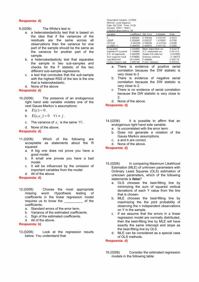
13. Look at the regression results below. You understand that:

a. There is evidence of positive serial correlation because the DW statistic is very close to 2

b. There is evidence of negative serial correlation because the DW statistic is very close to 2.

c. There is no evidence of serial correlation because the DW statistic is very close to 2.

d. None of the above. 14. It is possible to affirm that an endogenous

right hand side variable: a. Is uncorrelated with the error term. b. Does not generate a violation of the

Gauss Markov assumptions. c. a and b are correct. d. None of the above.

15. In comparing Maximum Likelihood Estimation (MLE) of unknown parameters with Ordinary Least Squares (OLS) estimation of unknown parameters, which of the following statements is false? a. OLS chooses the best-fitting line by

minimizing the sum of squared vertical deviations of each Y value from the line that is chosen.

b. MLE chooses the best-fitting line by maximizing the the joint probability of observing the n independent observations on Y in the sample.

c. If we assume that the errors in a linear regression model are normally distributed, then the best-fitting line by MLE will have exactly the same intercept and slope as the best-fitting line by OLS.

d. MLE can be considered as a special case of OLS methods.

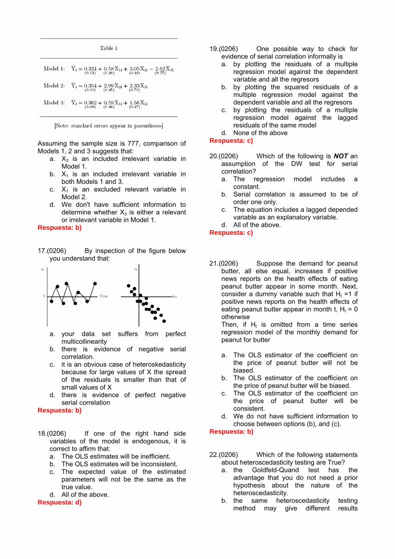
16. Consider the estimated regression models in the following table:



Assuming the sample size is 777, comparison of Models 1, 2 and 3 suggests that:

a. X3 is an included irrelevant variable in Model 1.

b. X1 is an included irrelevant variable in both Models 1 and 3.

c. X1 is an excluded relevant variable in Model 2.

d. We don't have sufficient information to determine whether X3 is either a relevant or irrelevant variable in Model 1.

17. By inspection of the figure below you understand that:

a. your data set suffers from perfect

multicollinearity b. there is evidence of negative serial

correlation. c. it is an obvious case of heteroskedasticity

because for large values of X the spread of the residuals is smaller than that of small values of X

d. there is evidence of perfect negative serial correlation

18. If one of the right hand side variables of the model is endogenous, it is correct to affirm that: a. The OLS estimates will be inefficient. b. The OLS estimates will be inconsistent. c. The expected value of the estimated

parameters will not be the same as the true value.

d. All of the above. 19. One possible way to check for evidence of

serial correlation informally is a. by plotting the residuals of a multiple

regression model against the dependent variable and all the regressors

b. by plotting the squared residuals of a multiple regression model against the dependent variable and all the regressors

c. by plotting the residuals of a multiple regression model against the lagged residuals of the same model

d. None of the above

20. Which of the following is NOT an assumption of the DW test for serial correlation? a. The regression model includes a

constant. b. Serial correlation is assumed to be of

order one only. c. The equation includes a lagged depended

variable as an explanatory variable. d. All of the above.

21. Suppose the demand for peanut butter, all else equal, increases if positive news reports on the health effects of eating peanut butter appear in some month. Next, consider a dummy variable such that Ht =1 if positive news reports on the health effects of eating peanut butter appear in month t, Ht = 0 otherwise Then, if Ht is omitted from a time series regression model of the monthly demand for peanut for butter a. The OLS estimator of the coefficient on

the price of peanut butter will not be biased.

b. The OLS estimator of the coefficient on the price of peanut butter will be biased.

c. The OLS estimator of the coefficient on the price of peanut butter will be consistent.

d. We do not have sufficient information to choose between options (b), and (c).

22. Which of the following statements about heteroscedasticity testing are True? a. the Goldfeld-Quand test has the

advantage that you do not need a prior hypothesis about the nature of the heteroscedasticity.

b. the same heteroscedasticity testing method may give different results depending on the functional form we choose.

c. a) and b) are correct d. None of the above.

23. Heteroscedasticty testing and tests for serial correlation have some things in common. Which of the following statements best describes the relationship between them: a. they are both performed on the basis of

estimates of the error term. b. some of them can be guaranteed to be

100% correct. c. All of the above. d. None of the above.



24. Which of the following reasons make OLS an imperfect choice of an estimation method when the dependent variable is a dummy variable? a. There will be a major heteroskedasticity

problem. b. If we interpret the fitted value of Y as the

probability of the 1 outcome, then for some sets of explanatory variable values, this fitted probability will be either negative or greater than one.

c. The conditional distribution of the Y variable, given a particular set of X values, is a two-valued discrete distribution, not a continuous approximately normal distribution.

d. All of the above. 25. It is possible to affirm that an instrumental

variable used in the estimation a model by 2 step least squares: a. is exogenous b. Is endogenous c. a and b may be correct d. None of the above.

26. Sean X y Z dos variables aleatorias, donde Z sólo puede tomar valores negativos, entonces E[XZ] es igual a: a. E[X ] E[Z ] b. E[X ] E[Z ] + Cov[X,Z] c. E[X ] E[Z ] - Cov[X,Z] d. - E[X ] E[Z ]

27. Las variables aleatorias X y Y tienen los siguientes momentos: ( ) 2E X = ; ( ) 3E Y = ;

( )2 13E X = ; ( )2 25E Y = ; ( ) 6E XY = . ¿Cuál de las siguientes afirmaciones es correcta?: a. ( ) ( )2 2 4− =E X E Y

b. ( ), 3Cov X Y =

c. X e Y no están correlacionadas

d. Si 2= +W X Y , entonces ( ) 9Var W =

28. Una buena razón para emplear los estimadores de mínimos cuadrados en dos etapas es: a. que exista autocorrelación en el término

aleatorio de error. b. que la variable dependiente (ceteris

paribus) sea medida con error. c. SIEMPRE que se estime una ecuación en

el contexto de un sistema de ecuaciones simultáneas.

d. Ninguna de las anteriores

29. Suponga el modelo yi = β1 + β1 xi + εi, en donde εi es el término de error, el cual es heteroscedástico con Var(εi) = αzi , donde zi es una variable observable y α es un término constante desconocido. El modelo que debería ser utilizado para corregir el problema de heteroscedasticidad es: a. yi zi = β1 zi + β2 xizi + εi* b. (yi/zi) = β1 (1/zi) + β2 (xi/zi) + εi* c. yi zi

1/2 = β1 zi1/2 + β2 xizi

1/2 + εi* d. (yi/zi

1/2) = β1 (1/zi1/2) + β2 (xi/zi

1/2) + εi*

30. ¿Cuál de las siguienstes afirmaciones es Falsa? a. Un coeficiente estimado numéricamente

pequeño puede ser estadísticamente significativo.

b. Un coeficiente estimado numéricamente pequeño puede ser estadísticamente NO significativo.

c. Un coeficiente estimado numéricamente grande puede ser estadísticamente significativo.

d. Todas las anteriores. 31. Suponga que la distribución muestral de un

estimador está CENTRADA EN el valor real del parámetro. En este contexto, centrada en significa que el estimador es: a. Eficiente. b. Sigue una distribución normal. c. Consistente. d. Ninguna de las anteriores.

32. La heteroscedasticidad en un modelo es un problema porque: a. El método MCO asume que los datos son

homoscedasticos y calcula estimadores puntuales de parámetros de la regresión de manera acorde.

b. El método MCO asume que los datos son homoscedasticos y calcula estimadores para los errores estándar de los parámetros de manera acorde.

c. Es contagioso. d. Sesga los estimadores puntuales de los

parámetros asociados con las pendientes e intercepto.

33. En un modelo de regresión lineal con una tendencia lineal (time trend), el coeficiente asociado a la tendencia puede ser: a. un estimador de la tasa de crecimiento %

de la variable dependiente (ceteris paribus).



b. El cambio en la variable dependiente por periodo de tiempo (ceteris paribus).

c. (a) y (b) pueden ser correctas. d. Ninguna de las anteriores.

34. Si se emplea los estimadores de MCO en presencia de heteroscedasticidad, pero emplea cuidadosamente la “fórmula” sugerida por White para calcular la varianza de los parámetros, entonces: a. Se tendrá el mejor valor estimado que se

pueda obtener, pues los MCO son MELI. b. Se tendrán valores estimados puntuales

insesgados para los parámetros, pero errores estándares con sesgo desconocido.

c. Se tendrán valores estimados puntuales insesgados para los parámetros, pero errores estándares que no son tan pequeños como los que se podrían obtener por medio del método de mínimos cuadrados ponderados.

d. Se estará cometiendo un grave error econométrico.

35. Considere la siguiente ecuación estimada: Yi = 2.22 – 0.25X1i + 0.76X2i - 0:03X3i; donde Y es la cantidad demandada del “bien 1”, X1 es el precio del “bien 1”, X2 es el precio del “bien 2” y X3 es el ingreso. Entonces, de acuerdo a la ecuación estimada: a. El bien 1 y el bien 2 son sustitutos. b. El bien 1 y el bien 2 son bienes

complementarios. c. El bien 1 es un bien normal. d. a) y c) son correctas.

36. En el modelo ( )0 1 1 2 21i iy X Xβ β β ε= + + + , se puede afirmar: a. 1β será negative si la relación entre y y

X1 es positiva. b. A medida que X1 aumenta y tiende a

0 2 2Xβ β+ c. 1β no corresponde ni a una elasticidad ni

al efecto marginal. d. Todas las anteriores.

37. Los Mínimos Cuadrados Generalizados (MCG)… a. Requieren del supuesto de

homoscedasticidad para ser MELI. b. Requieren del supuesto de no

autocorrelación para ser MELI. c. b y c son ciertos. d. Ninguna de las anteriores

38. ¿Cuál de los siguientes modelos muestra que el cambio en una unidad de X causa aproximadamente un incremento del 5% en y? a. y = 6 + 0.05 x b. y = 6 + 0.05 ln(x) c. ln(y) = 6 + 0.05 x d. ln(y) = 6 + 0.05 ln(x)

39. Comparando el método de Máxima Verosimilitud (MV) y el de Mínimos Cuadrados Ordinarios para la estimación de un modelo con variable dicotómica como dependiente, NO se puede afirmar que: a. MCO escoge la línea que mejor se ajusta

por medio de la minimización de la suma de las desviaciones cuadradas (en sentido vertical) de cada uno de los valores de Y con respecto a esta línea.

b. MV escoge la línea que mejor se ajusta maximizando la probabilidad conjunta de observar las n-observaciones independientes sobre Y en la muestra.

c. Si asumimos que los errores están normalmente distribuidos, entonces los valores estimados por MV serán iguales a los estimados por MCO.

d. Ninguna de las anteriores. 40. Un método informal usado para

comprobar la existencia de heteroscedasticidad es: a. Graficar los residuos de un modelo

de regresión múltiple contra todos los regresores.

b. Graficar los residuos de un modelo de regresión múltiple versus los residuos rezagados un período.

c. a) y b) son ciertas. d. ninguna de las anteriores.

41. Considere el siguiente modelo estimado: ˆ = 1.32 + 2.02 - 2.38 , i = 1,..., n,i i iH W C⋅ ⋅

donde Hi es el número de horas por semana laboradas por el trabajador i (medido en horas), Wi representa el salario (medidos en miles de pesos por hora) del trabajador i y Ci es el número de niños menores de 10 años que tiene el trabajador i. Entonces, de acuerdo a esta ecuación estimada de oferta de trabajo, si el trabajador i recibe $21,520 por hora y no tiene hijos, entonces el número de horas ofrecidas será (redondeando): a. 45.3 horas



b. 43.5 horas c. 44.8 horas d. 42.1 horas

42. Considere nuevamente el modelo estimado en la Pregunta 41. Para un aumento de una unidad tanto en el salario como en el número de niños y redondeando, la cantidad de trabajo ofrecido será: a. disminución de 0.36 horas. b. aumento de 0.63 horas. c. aumento de 4.40 horas. d. disminución de 5.72 horas.

43. De acuerdo al modelo estimado en la Pregunta 41, una mujer que acaba de dar a luz a dos mellizos: a. disminuirá su cantidad de trabajo

ofrecida en 4.76 horas. b. disminuirá su cantidad de trabajo

ofrecida en 2.38 horas. c. disminuirá su cantidad de trabajo

ofrecida en 1.19 horas. d. disminuirá su cantidad de trabajo

ofrecida en 7.14 horas. 44. Recuerde que la variable Wi en la Pregunta 41

está medida en miles de pesos por hora. Suponga que ahora la variable Wi fuera medida en pesos por hora. Entonces, el modelo estimado cambiará de la siguiente manera: a. el coeficiente estimado asociado con Wi

será 20.202. b. el coeficiente estimado asociado con Ci

será 23.802. c. el coeficiente estimado asociado con Wi

será 0.202. d. el coeficiente estimado asociado con Wi

será 0.0202. 45. Si se utiliza un computador para generar 60

observaciones y así construir una variable aleatoria (dependiente) Y, y de la misma forma se generan 60 observaciones para cincuenta variables independientes ( 1 2 50, ...X X X ). Entonces a. Una regresión de Y sobre estas 50

variables, con seguridad tendrá como resultado un R2 relativamente alto.

b. Una regresión de Y sobre estas 50 variables, tendrá con seguridad como resultado un intercepto igual al valor medio de Y.

c. Si se aplica minería de datos (data mining), se puede obtener que algunos coeficientes de pendiente son

estadísticamente significativos, pero estos resultados son espurios ya que por construcción se sabe que las pendientes son iguales a cero.

d. Si se aplica minería de datos (data mining), no es posible que se obtenga como resultado que las variables son significativas ya que por construcción las pendientes son iguales a cero.

46. Suponga que el verdadero modelo de regresión para la asistencia a los partidos de local del Deportivo Cali para la observación i incluye, entre otras variables explicatorias, tanto la probabilidad de lluvia para el periodo i y una variable dummy que toma el valor de 1 si el equipo visitante incluye una “super-estrella”. Si la variable dummy fuera excluida de la ecuación de regresión estimada y suponiendo que los fanáticos del Deportivo Cali les gusta ver jugar contra su equipo a “super-estrellas”, entonces el estimador MCO del coeficiente asociado a la probabilidad de lluvia será: a. MELI. b. sesgado. c. ineficiente d. b) y c) son correctas.

47. Los Mínimos Cuadrados Ponderados (MCP): a. Son un caso especial de los Mínimos

Cuadrados Ordinarios (MCO). b. Son un caso especial de los Mínimos

cuadrados generalizados c. Asignan una mayor influencia a las

observaciones donde los datos presentan mayor ruido (varianza), y una manor influencia a las observaciones donde los datos presentan menor ruido.

d. Requiere de variables adicionales en la formulación de MCO.

48. Una vez que ha sido estimado una especificación sensible para un modelo Logit o Probit: a. Se pueden interpretar los coeficientes

asociados a las pendientes como el cambio en la probabilidad de que la variable dependiente tome el valor de



1 causado por una unidad de cambio en esa variable X.

b. Se pueden interpretar los coeficientes estimados de las pendientes como el cambio en la propensión para elegir la variable dependiente que toma como valor 1.

c. No es posible calcular la derivada de la probabilidad de elegir a la variable dependiente que toma como valor 1, con respecto a una variable explicatoria X.

d. Ninguna de las anteriores. 49. Se sabe que dos estimadores para la

pendiente en un modelo de regresión simple ( 2β ) corresponden a

12 2

ˆ ˆ2 3Método MCOβ β= ⋅ y 22 2

ˆ ˆ1 3Método MCOβ β= ⋅ , donde 2

ˆ MCOβ es el correspondiente estimador de MCO y los otros estimadores corresponde a dos métodos diferentes., entonces se puede decir que: a. El estimador 3

2β̂ Método = 12β̂ Método +

22β̂ Método es un estimador consistente

de 2β . b. 1

2β̂ Método es un estimador con un sesgo mayor que 2

2β̂ Método . c. Tanto 1

2β̂ Método y 22β̂ Método son

estimadores eficientes de 2β . d. Ninguna de las anteriores.

50. Se sabe que el modelo real esta dado por yi=β1X1i+ β2X2i+ ε i , pero un investigador estima el siguiente modelo yi= β 1X1i+ ε i. con [(X2i)T(X1i)]≠0. Entonces: a. el estimador MCO no siempre es

sesgado. b. el estimador MCO siempre es

sesgado. c. el estimador MCO siempre es

concistente. . d. ninguna de las anteriores



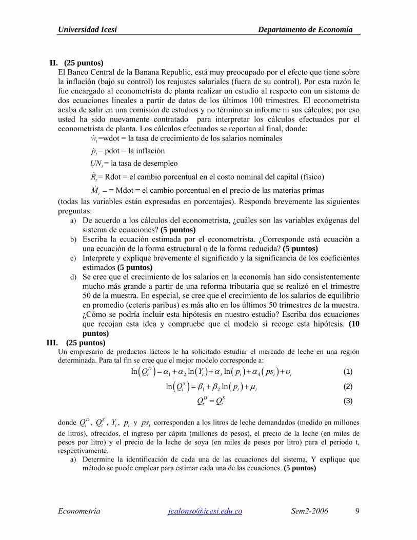
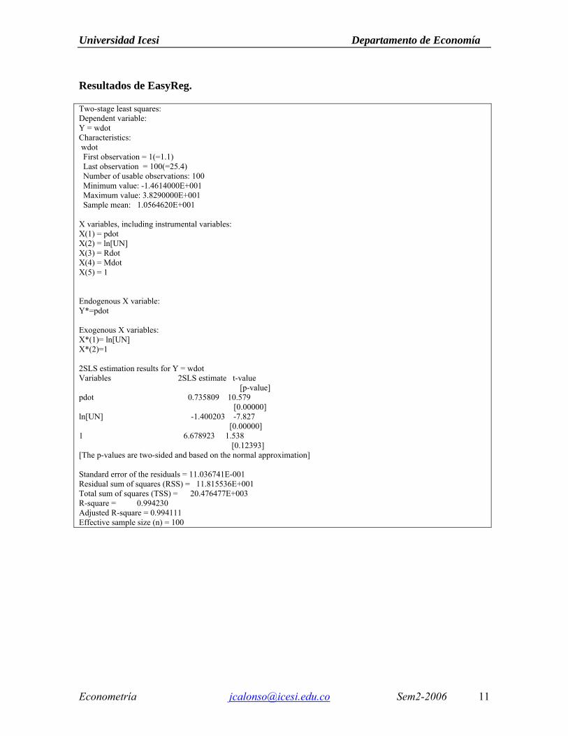
II. (25 puntos) El Banco Central de la Banana Republic, está muy preocupado por el efecto que tiene sobre la inflación (bajo su control) los reajustes salariales (fuera de su control). Por esta razón le fue encargado al econometrista de planta realizar un estudio al respecto con un sistema de dos ecuaciones lineales a partir de datos de los últimos 100 trimestres. El econometrista acaba de salir en una comisión de estudios y no término su informe ni sus cálculos; por eso usted ha sido nuevamente contratado para interpretar los cálculos efectuados por el econometrista de planta. Los cálculos efectuados se reportan al final, donde:

=wdot = la tasa de crecimiento de los salarios nominales= pdot = la inflación

= la tasa de desempleo

= Rdot = el cambio porcentual en el costo nominal del capital (físico)

= Mdot = el ca

t

t

t

t

t

wpUN

R

M = mbio porcentual en el precio de las materias primas

(todas las variables están expresadas en porcentajes). Responda brevemente las siguientes preguntas:

a) De acuerdo a los cálculos del econometrista, ¿cuáles son las variables exógenas del sistema de ecuaciones? (5 puntos)

b) Escriba la ecuación estimada por el econometrista. ¿Corresponde está ecuación a una ecuación de la forma estructural o de la forma reducida? (5 puntos)

c) Interprete y explique brevemente el significado y la significancia de los coeficientes estimados (5 puntos)

d) Se cree que el crecimiento de los salarios en la economía han sido consistentemente mucho más grande a partir de una reforma tributaria que se realizó en el trimestre 50 de la muestra. En especial, se cree que el crecimiento de los salarios de equilibrio en promedio (ceteris paribus) es más alto en los últimos 50 trimestres de la muestra. ¿Cómo se podría incluir esta hipótesis en nuestro estudio? Escriba dos ecuaciones que recojan esta idea y compruebe que el modelo si recoge esta hipótesis. (10 puntos)

III. (25 puntos) Un empresario de productos lácteos le ha solicitado estudiar el mercado de leche en una región determinada. Para tal fin se cree que el mejor modelo corresponde a: ( ) ( ) ( ) ( )1 2 3 4ln ln lnD

t t t t tQ Y p psα α α α υ= + + + + (1)

( ) ( )1 2ln lnSt t tQ pβ β μ= + + (2)

D St tQ Q= (3)

donde D

tQ , StQ , tY , tp y tps corresponden a los litros de leche demandados (medido en millones

de litros), ofrecidos, el ingreso per cápita (millones de pesos), el precio de la leche (en miles de pesos por litro) y el precio de la leche de soya (en miles de pesos por litro) para el periodo t, respectivamente.

a) Determine la identificación de cada una de las ecuaciones del sistema, Y explique que método se puede emplear para estimar cada una de las ecuaciones. (5 puntos)



Una de sus primeras tareas en este estudio será estimar la expresión describe el comportamiento del precio de equilibrio. Para esto su asisten le ha preparado las siguientes matrices:

100 0 0

80 040

TX X⎡ ⎤⎢ ⎥= ⎢ ⎥⎢ ⎥⎣ ⎦

5

1608

TX y⎡ ⎤⎢ ⎥= ⎢ ⎥⎢ ⎥⎣ ⎦

b) Escriba la respectiva ecuación que deberá estimar y explique claramente a que corresponde cada uno de los elementos de la matriz TX X . (Por ejemplo, explique a partir de que sumatoria sale el 40 que corresponde al último elemento de la matriz

TX X , y así sucesivamente con cada elemento de la matriz) (5 puntos ) c) ¿Qué método se debe emplear y que supuestos se deben cumplir para que los estimadores

de los parámetros del modelo que corresponde al precio de equilibrio sea MELI? (5 Puntos)

d) Estime los coeficientes del modelo que corresponde al precio de equilibrio. (5 Puntos) e) Interprete el significado de cada uno de los coeficientes estimados.(5 Puntos)



Resultados de EasyReg. Two-stage least squares: Dependent variable: Y = wdot Characteristics: wdot First observation = 1(=1.1) Last observation = 100(=25.4) Number of usable observations: 100 Minimum value: -1.4614000E+001 Maximum value: 3.8290000E+001 Sample mean: 1.0564620E+001 X variables, including instrumental variables: X(1) = pdot X(2) = ln[UN] X(3) = Rdot X(4) = Mdot X(5) = 1 Endogenous X variable: Y*=pdot Exogenous X variables: X*(1)= ln[UN] X*(2)=1 2SLS estimation results for Y = wdot Variables 2SLS estimate t-value [p-value] pdot 0.735809 10.579 [0.00000] ln[UN] -1.400203 -7.827 [0.00000] 1 6.678923 1.538 [0.12393] [The p-values are two-sided and based on the normal approximation] Standard error of the residuals = 11.036741E-001 Residual sum of squares (RSS) = 11.815536E+001 Total sum of squares (TSS) = 20.476477E+003 R-square = 0.994230 Adjusted R-square = 0.994111 Effective sample size (n) = 100

Econometría, Examen Parcial II

Prof: Julio César Alonso C

Fórmulas

1 21 1 1

21 1 2 1

1 1 1

22 2

1 1

2

1

n n n

i i kii i in n n

i i i i kii i i

T n n

i i kii i

n

kii

n X X X

X X X X X

X XX X X

X

= = =

= = =

= =

=

⎡ ⎤⎢ ⎥⎢ ⎥⎢ ⎥⎢ ⎥⎢ ⎥

= ⎢ ⎥⎢ ⎥⎢ ⎥⎢ ⎥⎢ ⎥⎢ ⎥⎢ ⎥⎣ ⎦

∑ ∑ ∑

∑ ∑ ∑

∑ ∑

∑

1

11

21

1

n

ii

n

i ii

T n

i ii

n

i kii

y

y X

X yy X

y X

=

=

=

=

⎡ ⎤⎢ ⎥⎢ ⎥⎢ ⎥⎢ ⎥⎢ ⎥

= ⎢ ⎥⎢ ⎥⎢ ⎥⎢ ⎥⎢ ⎥⎢ ⎥⎢ ⎥⎣ ⎦

∑

∑

∑

∑

2

1

nT

ii

y y y=

= ∑

( )2 2

1

nT

ii

SST y y y y nY=

= − = −∑ ( )2

1

ˆn

i ii

SSE y y=

= −∑

( ) 1ˆ T TX X X yβ−

= 2ˆT T TSSE y y X ys

n k n kβ−

= =− −

( ) 12ˆ TVar X Xβ σ−⎡ ⎤ =⎣ ⎦

( )2 2

1

ˆˆn

T Ti

iSSR y y X y nYβ

=

= − = −∑ ˆ

ˆ

i

i ctsβ

β −=

( ) ( )( ) ( )11ˆ ˆT

T T

c

c R R X X R c R rF

SSE n k

β β−−

− −=

−

( )( )

2

2

11 ( )C

R k MSRFMSER n k

−= =

− −

( )( )

R Uc

U

SSE SSE rF

SSE n k−

=−

2 SSRRSST

=

ˆ,

2

ˆi

i n kt sα β

β−

± ( )2 2 11 1 nR Rn k−

= − −−

( )1 2ˆˆ , 1T T

p p p p p kpy x x x x xβ= = …

( ) 12

,2

ˆ T Tp p pn k

y t x X X xα σ−

−±

( ) 12

,2

ˆ 1 T Tp p pn k

y t x X X xα σ−

−

⎡ ⎤± +⎢ ⎥⎣ ⎦

ˆ ˆ , 2,3, ,jXEj j

y

sj k

sβ β= = … ˆ j

j j

XE

yβ=

Econometría, Examen Parcial II

Prof: Julio César Alonso C

Test de Heteroscedasticidad

Goldfeld y Quand: ( )2

2 , 21

GQ n d k n d k

SSEF F

SSE − − − −= ∼

Breush-Pagan: 2

2

ˆˆi

i iZε

γ δ µσ

= + + , 2

2 gSSRBP χ= ∼

White: 2

1 1

ˆk k

i s mi ji im j

X Xε γ δ µ= =

= + +∑∑ , 2 2a gW nR χ= ∼

Test de Autocorrelación

Durbin-Watson ( )ˆ2 1DW ρ≈ − Ho Sí Decisión

0 : 0H ρ = 4u ud DW d< < − A No auto + 0 lDW d< < R No auto - 4 4ld DW− < < R Área de indecisión l ud DW d< < y 4 4u ld DW d− < < −

Cantidades Importantes

2 1.414= 3 1.732=10 3.162= 13 3.606=

dl y du para el test de DW al nivel de significancia del 5% N k-1=1 k-1=2 k-1=3 dl du dl du dl du 50 1.50 1.59 1.46 1.63 1.42 1.6760 1.55 1.62 1.51 1.65 1.48 1.6995 1.64 1.69 1.62 1.71 1.60 1.73100 1.65 1.69 1.63 1.72 1.61 1.74 Condición de Orden

1i ik g> − sobre-identificada 1i ik g= − perfectamente identificada

HOJA DE RESPUESTAS PREGUNTAS DE SELECCIÓN MÚLTIPLE NOMBRE:__________________________________

En está hoja marque la respuesta correcta. A B C D 1. O O O O 2. O O O O 3. O O O O 4. O O O O 5. O O O O 6. O O O O 7. O O O O 8. O O O O 9. O O O O 10. O O O O 11. O O O O 12. O O O O 13. O O O O 14. O O O O 15. O O O O 16. O O O O 17. O O O O 18. O O O O 19. O O O O 20. O O O O 21. O O O O 22. O O O O 23. O O O O 24. O O O O 25. O O O O

A B C D 26. O O O O 27. O O O O 28. O O O O 29. O O O O 30. O O O O 31. O O O O 32. O O O O 33. O O O O 34. O O O O 35. O O O O 36. O O O O 37. O O O O 38. O O O O 39. O O O O 40. O O O O 41. O O O O 42. O O O O 43. O O O O 44. O O O O 45. O O O O 46. O O O O 47. O O O O 48. O O O O 49. O O O O 50. O O O O

Sem2-2006 I. Selección Múltiple (50 puntos en total, 1

punto por cada subparte) Seleccione la opción más indicada en la hoja de respuestas que encontrará al final de este examen. Sólo se considerarán respuestas que sean consignadas en la hoja de respuestas. (No es necesario justificar su respuesta) 1.(0206) Consider the following population

regression model:

0 1 1 2 2i iY X X i iβ β β= + + +ε

and assume that 1 85i iX = × 2X for each observation i. Then a. the stochastic error term is de_nitely

homoskedastic. b. the stochastic error term is de_nitely

heteroskedastic. c. the observations of the stochastic error

term are de_nitely serially correlated. d. the parameters of this model can not be

estimated by OLS. Respuesta: d)

2.(0206) If your dataset has serial

correlation, but you completely ignore the problem and estimate a linear model by OLS, you will: a. get biased parameter estimates. b. you get OLS estimators that are still

BLUE. c. get t-test statistics that make you reject

the null hypothesis about the overall significance of the model.

d. None of the above. Respuesta: d)

3.(0206) Good ways to deal with multicollinearity include: a. getting additional data, where the

collinearities between your regressors may not be as strong.

b. using outside information about the relationship between coefficients on collinear variables to reduce the number of slope parameters to be estimated.

c. dropping one of the multicollinear variables from your regression model.

d. all except c. Respuesta: d)

4.(0206) Which of the following assumptions related to the distribution of the error term corresponds to a probit model: a. The error term follows a normal

distribution. b. The error term follows a logistic

distribution

c. The error term follows a chi-square distribution.

d. None of the above. Respuesta: a)

5.(0206) Comparing the three functional forms:

Which of the following statements are true: a. of the three, A always has the highest

values for b1 with B having the second highest.

b. all of the three could have a negative value for the intercept in the estimated equation.

c. of the three, A always has the highest elasticity’s with B having the second highest.

d. None of the above. Respuesta: b)

6.(0206) Choose the most appropriate words to fill in the blanks. "The disturbance term in a regression equation measures, amongst other things, the influence of ________ on the _______ model.": a. Omitted variables/specified. b. Measurement errors in Y /theoretical. c. Omitted variables/theoretical. d. The included variables/specified.

Respuesta: a)

7.(0206) A regression equation can be checked for stability using which of the following: a. Chow test. b. Durbin-Watson test. c. R squared being too high. d. None of the above.

Respuesta: a)

8.(0206) The relationship between the R squared and the F for the equation is as follows a. A large R squared must mean a large and

significant F test b. R squared goes up when we add

variables but the statistical significance Of the F ratio may go down

c. Once we know the R squared, there can only be one valued of the F test. As they both use the same set of information (sum of squared residuals).

d. (b) and (c) are correct.

Respuesta: d)

9.(0206) The White’s test is: a. a heteroskedasticity test that is based on

the idea that if the variances of the residuals are the same across all observations then the variance for one part of the sample should be the same as the variance for another part of the sample.

b. a heteroskedasticity test that separates the sample in two sub-samples and checks for the F statistic of the two different sub-sample regressions.

c. a test that concludes that the sub-sample with the highest RSS of the two is the one that is heteroskedastic.

d. None of the above Respuesta: d)

10.(0206) The presence of an endogenous right hand side variable violates one of the next Gauss-Markov´s assumptions: a. ( ) 0E ε = .

b. ( ) 0i jE i jε ε = ∀ ≠ .

c. The variance of iε is the same . i∀d. None of the above.

Respuesta: d)

11.(0206) Which of the following are acceptable as statements about the R squared: a. A big one does not prove you have a

good model. b. A small one proves you have a bad

model. c. It will be influenced by the omission of

important variables from the model d. All of the above.

Respuesta: d)

12.(0206) Choose the most appropriate

missing word: Hypothesis testing of coefficients in the linear regression model requires us to know the __________ of the coefficients: a. Standard errors of the error term. b. Variance of the estimated coefficients. c. Sign of the estimated coefficients. d. All of the above.

Respuesta: b)

13.(0206) Look at the regression results below. You understand that:

a. There is evidence of positive serial

correlation because the DW statistic is very close to 2

b. There is evidence of negative serial correlation because the DW statistic is very close to 2.

c. There is no evidence of serial correlation because the DW statistic is very close to 2.

d. None of the above. Respuesta: d)

14.(0206) It is possible to affirm that an endogenous right hand side variable: a. Is uncorrelated with the error term. b. Does not generate a violation of the

Gauss Markov assumptions. c. a and b are correct. d. None of the above.

Respuesta: d)

15.(0206) In comparing Maximum Likelihood Estimation (MLE) of unknown parameters with Ordinary Least Squares (OLS) estimation of unknown parameters, which of the following statements is false? a. OLS chooses the best-fitting line by

minimizing the sum of squared vertical deviations of each Y value from the line that is chosen.

b. MLE chooses the best-fitting line by maximizing the the joint probability of observing the n independent observations on Y in the sample.

c. If we assume that the errors in a linear regression model are normally distributed, then the best-fitting line by MLE will have exactly the same intercept and slope as the best-fitting line by OLS.

d. MLE can be considered as a special case of OLS methods.

Respuesta: d)

16.(0206) Consider the estimated regression

models in the following table:

Assuming the sample size is 777, comparison of Models 1, 2 and 3 suggests that:

a. X3 is an included irrelevant variable in Model 1.

b. X1 is an included irrelevant variable in both Models 1 and 3.

c. X1 is an excluded relevant variable in Model 2.

d. We don't have sufficient information to determine whether X3 is either a relevant or irrelevant variable in Model 1.

Respuesta: b)

17.(0206) By inspection of the figure below

you understand that:

a. your data set suffers from perfect

multicollinearity b. there is evidence of negative serial

correlation. c. it is an obvious case of heteroskedasticity

because for large values of X the spread of the residuals is smaller than that of small values of X

d. there is evidence of perfect negative serial correlation

Respuesta: b)

18.(0206) If one of the right hand side

variables of the model is endogenous, it is correct to affirm that: a. The OLS estimates will be inefficient. b. The OLS estimates will be inconsistent. c. The expected value of the estimated

parameters will not be the same as the true value.

d. All of the above. Respuesta: d)

19.(0206) One possible way to check for

evidence of serial correlation informally is a. by plotting the residuals of a multiple

regression model against the dependent variable and all the regresors

b. by plotting the squared residuals of a multiple regression model against the dependent variable and all the regresors

c. by plotting the residuals of a multiple regression model against the lagged residuals of the same model

d. None of the above Respuesta: c)

20.(0206) Which of the following is NOT an assumption of the DW test for serial correlation? a. The regression model includes a

constant. b. Serial correlation is assumed to be of

order one only. c. The equation includes a lagged depended

variable as an explanatory variable. d. All of the above.

Respuesta: c)

21.(0206) Suppose the demand for peanut

butter, all else equal, increases if positive news reports on the health effects of eating peanut butter appear in some month. Next, consider a dummy variable such that Ht =1 if positive news reports on the health effects of eating peanut butter appear in month t, Ht = 0 otherwise Then, if Ht is omitted from a time series regression model of the monthly demand for peanut for butter

a. The OLS estimator of the coefficient on

the price of peanut butter will not be biased.

b. The OLS estimator of the coefficient on the price of peanut butter will be biased.

c. The OLS estimator of the coefficient on the price of peanut butter will be consistent.

d. We do not have sufficient information to choose between options (b), and (c).

Respuesta: b)

22.(0206) Which of the following statements

about heteroscedasticity testing are True? a. the Goldfeld-Quand test has the

advantage that you do not need a prior hypothesis about the nature of the heteroscedasticity.

b. the same heteroscedasticity testing method may give different results

depending on the functional form we choose.

c. a) and b) are correct d. None of the above.

Respuesta: b)

23.(0206) Heteroscedasticty testing and

tests for serial correlation have some things in common. Which of the following statements best describes the relationship between them: a. they are both performed on the basis of

estimates of the error term. b. some of them can be guaranteed to be

100% correct. c. All of the above. d. None of the above.

Respuesta: a)

24.(0206) Which of the following reasons

make OLS an imperfect choice of an estimation method when the dependent variable is a dummy variable? a. There will be a major heteroskedasticity

problem. b. If we interpret the fitted value of Y as the

probability of the 1 outcome, then for some sets of explanatory variable values, this fitted probability will be either negative or greater than one.

c. The conditional distribution of the Y variable, given a particular set of X values, is a two-valued discrete distribution, not a continuous approximately normal distribution.

d. All of the above. Respuesta: d)

25.(0206) It is possible to affirm that an

instrumental variable used in the estimation a model by 2 step least squares: a. is exogenous b. Is endogenous c. a and b may be correct d. None of the above.

Respuesta: a)

26.(0206) Sean X y Z dos variables

aleatorias, donde Z sólo puede tomar valores negativos, entonces E[XZ] es igual a: a. E[X ] E[Z ] b. E[X ] E[Z ] + Cov[X,Z] c. E[X ] E[Z ] - Cov[X,Z] d. - E[X ] E[Z ]

Respuesta: b)

27.(0206) Las variables aleatorias X y Y tienen los siguientes momentos: ( ) 2E X = ;

( ) 3E Y = ; ( )2 13E X = ; ( )2 25E Y = ;

( ) 6E XY = . ¿Cuál de las siguientes afirmaciones es correcta?: a. ( ) ( )2 2 4− =E X E Y

b. ( ), 3Cov X Y = c. X e Y no están correlacionadas d. Si 2= +W X Y , entonces ( ) 9Var W =

Respuesta: c)

28.(0206) Una buena razón para emplear los estimadores de mínimos cuadrados en dos etapas es: a. que exista autocorrelación en el término

aleatorio de error. b. que la variable dependiente (ceteris

paribus) sea medida con error. c. SIEMPRE que se estime una ecuación en

el contexto de un sistema de ecuaciones simultáneas.

d. Ninguna de las anteriores Respuesta: d)

29.(0206) Suponga el modelo yi = β1 + β1 xi

+ εi, en donde εi es el término de error, el cual es heteroscedástico con Var(εi) = αzi , donde zi es una variable observable y α es un término constante desconocido. El modelo que debería ser utilizado para corregir el problema de heteroscedasticidad es:

a. yi zi = β1 zi + β2 xizi + εi* b. (yi/zi) = β1 (1/zi) + β2 (xi/zi) + εi* c. yi zi

1/2 = β1 zi1/2 + β2 xizi

1/2 + εi* d. (yi/zi

1/2) = β1 (1/zi1/2) + β2 (xi/zi

1/2) + εi* Respuesta: d)

30.(0206) ¿Cuál de las siguientes afirmaciones es Falsa? a. Un coeficiente estimado numéricamente

pequeño puede ser estadísticamente significativo.

b. Un coeficiente estimado numéricamente pequeño puede ser estadísticamente NO significativo.

c. Un coeficiente estimado numéricamente grande puede ser estadísticamente significativo.

d. Todas las anteriores. Respuesta: d)

31.(0206) Suponga que la distribución muestral de un estimador está CENTRADA EN el valor real del parámetro. En este

contexto, centrada en significa que el estimador es: a. Eficiente. b. Sigue una distribución normal. c. Consistente. d. Ninguna de las anteriores.

Respuesta: d)

32.(0206) La heteroscedasticidad en un modelo es un problema porque: a. El método MCO asume que los datos son

homoscedásticos y calcula estimadores puntuales de parámetros de la regresión de manera acorde.

b. El método MCO asume que los datos son homoscedásticos y calcula estimadores para los errores estándar de los parámetros de manera acorde.

c. Es contagioso. d. Sesga los estimadores puntuales de los

parámetros asociados con las pendientes e intercepto.

Respuesta: b)

33.(0206) En un modelo de regresión lineal con una tendencia lineal (time trend), el coeficiente asociado a la tendencia puede ser: a. un estimador de la tasa de crecimiento %

de la variable dependiente (ceteris paribus).

b. El cambio en la variable dependiente por periodo de tiempo (ceteris paribus).

c. (a) y (b) pueden ser correctas. d. Ninguna de las anteriores.

Respuesta: c)

34.(0206) Si se emplea los estimadores de MCO en presencia de heteroscedasticidad, pero emplea cuidadosamente la “fórmula” sugerida por White para calcular la varianza de los parámetros, entonces: a. Se tendrá el mejor valor estimado que se

pueda obtener, pues los MCO son MELI. b. Se tendrán valores estimados puntuales

insesgados para los parámetros, pero errores estándares con sesgo desconocido.

c. Se tendrán valores estimados puntuales insesgados para los parámetros, pero errores estándares que no son tan pequeños como los que se podrían obtener por medio del método de mínimos cuadrados ponderados.

d. Se estará cometiendo un grave error econométrico.

Respuesta: c)

35.(0206) Considere la siguiente ecuación estimada: Yi = 2.22 – 0.25X1i + 0.76X2i - 0:03X3i;

donde Y es la cantidad demandada del “bien 1”, X1 es el precio del “bien 1”, X2 es el precio del “bien 2” y X3 es el ingreso. Entonces, de acuerdo a la ecuación estimada: a. El bien 1 y el bien 2 son sustitutos. b. El bien 1 y el bien 2 son bienes

complementarios. c. El bien 1 es un bien normal. d. a) y c) son correctas.

Respuesta: a)

36.(0206) En el modelo ( )0 1 1 2 21i iy X Xβ β β ε= + + + , se puede

afirmar: a. 1β será negativa si la relación entre y y

X1 es positiva. b. A medida que X1 aumenta y tiende a

0 2 2Xβ β+ c. 1β no corresponde ni a una elasticidad ni

al efecto marginal. d. Todas las anteriores.

Respuesta: d)

37.(0206) Los Mínimos Cuadrados Generalizados (MCG)… a. Requieren del supuesto de

homoscedasticidad para ser MELI. b. Requieren del supuesto de no

autocorrelación para ser MELI. c. b y c son ciertos. d. Ninguna de las anteriores Respuesta: d)

38.(0206) ¿Cuál de los siguientes modelos muestra que el cambio en una unidad de X causa aproximadamente un incremento del 5% en y? a. y = 6 + 0.05 x b. y = 6 + 0.05 ln(x) c. ln(y) = 6 + 0.05 x d. ln(y) = 6 + 0.05 ln(x)

Respuesta: c 39.(0206) Comparando el método de

Máxima Verosimilitud (MV) y el de Mínimos Cuadrados Ordinarios para la estimación de un modelo con variable dicotómica como dependiente, NO se puede afirmar que: a. MCO escoge la línea que mejor se ajusta

por medio de la minimización de la suma de las desviaciones cuadradas (en sentido vertical) de cada uno de los valores de Y con respecto a esta línea.

b. MV escoge la línea que mejor se ajusta maximizando la probabilidad conjunta de observar las n-observaciones independientes sobre Y en la muestra.

c. Si asumimos que los errores están normalmente distribuidos, entonces los valores estimados por MV serán iguales a los estimados por MCO.

d. Ninguna de las anteriores. Respuesta: c 40.(0206) Un método informal usado para

comprobar la existencia de heteroscedasticidad es: a. Graficar los residuos de un modelo de

regresión múltiple contra todos los regresores.

b. Graficar los residuos de un modelo de regresión múltiple versus los residuos rezagados un período.

c. a) y b) son ciertas. d. ninguna de las anteriores.

Respuesta: a)

41.(0206) Considere el siguiente modelo estimado:

donde H

ˆ = 1.32 + 2.02 - 2.38 , i = 1,..., n,i i iH W C⋅ ⋅

i es el número de horas por semana laboradas por el trabajador i (medido en horas), Wi representa el salario (medidos en miles de pesos por hora) del trabajador i y Ci es el número de niños menores de 10 años que tiene el trabajador i. Entonces, de acuerdo a esta ecuación estimada de oferta de trabajo, si el trabajador i recibe $21,520 por hora y no tiene hijos, entonces el número de horas ofrecidas será (redondeando): a. 45.3 horas b. 43.5 horas c. 44.8 horas d. 42.1 horas

Respuesta: c)

42.(0206) Considere nuevamente el modelo

estimado en la Pregunta 41.(0206). Para un aumento de una unidad tanto en el salario como en el número de niños y redondeando, la cantidad de trabajo ofrecido será: a. disminución de 0.36 horas. b. aumento de 0.63 horas. c. aumento de 4.40 horas. d. disminución de 5.72 horas.

Respuesta: a)

43.(0206) De acuerdo al modelo estimado

en la Pregunta 41.(0206), una mujer que acaba de dar a luz a dos mellizos: a. disminuirá su cantidad de trabajo ofrecida

en 4.76 horas. b. disminuirá su cantidad de trabajo ofrecida

en 2.38 horas. c. disminuirá su cantidad de trabajo ofrecida

en 1.19 horas. d. disminuirá su cantidad de trabajo ofrecida

en 7.14 horas. Respuesta: a)

44.(0206) Recuerde que la variable Wi en la Pregunta 41.(0206) está medida en miles de pesos por hora. Suponga que ahora la variable Wi fuera medida en pesos por hora. Entonces, el modelo estimado cambiará de la siguiente manera: a. el coeficiente estimado asociado con Wi

será 20.202. b. el coeficiente estimado asociado con Ci

será 23.802. c. el coeficiente estimado asociado con Wi

será 0.00202. d. el coeficiente estimado asociado con Wi

será 0.0202.

Respuesta: c)

45.(0206) Si se utiliza un computador para generar 60 observaciones y así construir una variable aleatoria (dependiente) Y, y de la misma forma se generan 60 observaciones para cincuenta variables independientes ( 1 2 5, ... 0X X X ). Entonces a. Una regresión de Y sobre estas 50

variables, con seguridad tendrá como resultado un R2 relativamente alto.

b. Una regresión de Y sobre estas 50 variables, tendrá con seguridad como resultado un intercepto igual al valor medio de Y.

c. Si se aplica minería de datos (data mining), se puede obtener que algunos coeficientes de pendiente son estadísticamente significativos, pero estos resultados son espurios ya que por construcción se sabe que las pendientes son iguales a cero.

d. Si se aplica minería de datos (data mining), no es posible que se obtenga como resultado que las variables son significativas ya que por construcción las pendientes son iguales a cero.

Respuesta: c)

46.(0206) Suponga que el verdadero modelo de regresión para la asistencia a los partidos de local del Deportivo Cali para la observación i incluye, entre otras variables explicatorias, tanto la probabilidad de lluvia para el periodo i y una variable dummy que toma el valor de 1 si el equipo visitante incluye una “super-estrella”. Si la variable dummy fuera excluida de la ecuación de regresión estimada y suponiendo que los fanáticos del Deportivo Cali les gusta ver jugar contra su equipo a “super-estrellas”, entonces el estimador MCO del coeficiente asociado a la probabilidad de lluvia será: a. MELI. b. sesgado.

c. ineficiente 50.(0206) Se sabe que el modelo real esta dado por yi=�0+�1X1i+ �2X2i+ � i , pero un investigador estima el siguiente modelo yi=�0+� 1X1i+ � i. con [(X2i)T(X1i)]≠0. Entonces:

d. b) y c) son correctas. Respuesta: a)

47.(0206) Los Mínimos Cuadrados Ponderados (MCP): a. el estimador MCO no siempre es

sesgado. a. Son un caso especial de los Mínimos Cuadrados Ordinarios (MCO). b. el estimador MCO siempre es sesgado.

c. el estimador MCO siempre es consistente. .

b. Son un caso especial de los Mínimos cuadrados generalizados

d. ninguna de las anteriores c. Asignan una mayor influencia a las observaciones donde los datos presentan mayor ruido (varianza), y una manor influencia a las observaciones donde los datos presentan menor ruido.

Respuesta:a)

d. Requiere de variables adicionales en la formulación de MCO.

Respuesta: b)

48.(0206) Una vez que ha sido estimado una especificación sensible para un modelo Logit o Probit: a. Se pueden interpretar los coeficientes

asociados a las pendientes como el cambio en la probabilidad de que la variable dependiente tome el valor de 1 causado por una unidad de cambio en esa variable X.

b. Se pueden interpretar los coeficientes estimados de las pendientes como el cambio en la propensión para elegir la variable dependiente que toma como valor 1.

c. No es posible calcular la derivada de la probabilidad de elegir a la variable dependiente que toma como valor 1, con respecto a una variable explicatoria X.

d. Ninguna de las anteriores. Respuesta: d)

49.(0206) Se sabe que dos estimadores para la pendiente en un modelo de regresión simple ( 2β ) corresponden a

12 2

ˆ ˆ2 3Método MCOβ β= ⋅ y 22 2

ˆ ˆ1 3Método MCOβ β= ⋅ ,

donde 2ˆ MCOβ es el correspondiente estimador

de MCO y los otros estimadores corresponde a dos métodos diferentes., entonces se puede decir que: a. El estimador 3

2β̂Método = 1

2β̂Método + 2

2β̂Método

es un estimador consistente de 2β .

b. 12β̂Método es un estimador con un sesgo

mayor que 22β̂Método .

c. Tanto 12β̂Método y 2

2β̂Método son estimadores

eficientes de 2β . d. Ninguna de las anteriores.

Respuesta: a)

II. (25 puntos) El Banco Central de la Banana Republic, está muy preocupado por el efecto que tiene sobre la inflación (bajo su control) los reajustes salariales (fuera de su control). Por esta razón le fue encargado al econometrista de planta realizar un estudio al respecto con un sistema de dos ecuaciones lineales a partir de datos de los últimos 100 trimestres. El econometrista acaba de salir en una comisión de estudios y no término su informe ni sus cálculos; por eso usted ha sido nuevamente contratado para interpretar los cálculos efectuados por el econometrista de planta. Los cálculos efectuados se reportan al final, donde:

=wdot = la tasa de crecimiento de los salarios nominales= pdot = la inflación

= la tasa de desempleo

= Rdot = el cambio porcentual en el costo nominal del capital (físico)

= Mdot = el ca

t

t

t

t

t

wpUN

R

M = mbio porcentual en el precio de las materias primas

(todas las variables están expresadas en porcentajes). Responda brevemente las siguientes preguntas: a) De acuerdo a los cálculos del econometrista, ¿cuáles son las variables exógenas del sistema de

ecuaciones? (5 puntos) Las variables exógenas del sistema de ecuaciones son: [ ]ln tUN , tR y tM

b) Escriba la ecuación estimada por el econometrista. ¿Corresponde está ecuación a una ecuación de la forma estructural o de la forma reducida? (5 puntos)

wdothati 6.679 1.40 ln UNi( )⋅− 0.736 pdoti⋅+ Esta ecuación corresponde a la forma estructural

c) Interprete y explique brevemente el significado y la significancia de los coeficientes estimados (5 puntos)

αhat0 =6.679% no tiene interpretación económica. Este coeficiente no es significativo.

αhat1 = -1.40. Un aumento de un uno por ciento de la tasa de desempleo disminuirá la tasa de crecimiento de los salarios en 0.014(1.4/100) puntos porcentuales. Note que este coeficiente tiene el signo esperado. Este coeficiente es significativo a un nivel del 1% de significancia. αhat2 = 0.736. Un aumento en un punto porcentual en la inflación provocará un aumento de 0.736 puntos porcentuales en la tasa de crecimiento de los salarios. Note que este coeficiente tiene el signo esperado. Este coeficiente es significativo a un nivel del 1% de significancia. (0.5 puntos por la significancia, el resto por la interpretación)

d) Se cree que el crecimiento de los salarios en la economía han sido consistentemente mucho más grande a partir de una reforma tributaria que se realizó en el trimestre 50 de la muestra. En especial, se cree que el crecimiento de los salarios de equilibrio en promedio (ceteris paribus) es más alto en los últimos 50 trimestres de la muestra. ¿Cómo se podría incluir esta hipótesis en nuestro estudio? Escriba la ecuación que recoja esta idea y compruebe que el modelo sí recoge esta hipótesis. (10 puntos)

Para capturar esta hipótesis creemos la siguiente variable dummy:

1 i >50 . .i

siD

o w⎧

= ⎨⎩

0

Así la forma reducida que explica el crecimiento de los salarios de equilibrio sería: wdoti π11 π12 ln UNi( )⋅+ π13 Rdoti⋅+ π14 Mdoti⋅+ π15 Di⋅+ εi+ Para demostrar que el modelo anterior si captura la hipótesis, se requiere calcular el valor esperado de la ecuación.

[ ] [ ][ ]

11 15 12 13 14

11 12 13 14

ln i 50ln . .

t i

t i

UN Rdot Mdot siE wdoti

UN Rdot Mdot o wπ π π π ππ π π π

⎧ + + + + >⎪= ⎨ + + +⎪⎩

Luego el modelo si captura la hipótesis.

III. (25 puntos) Un empresario de productos lácteos le ha solicitado estudiar el mercado de leche en una región determinada. Para tal fin se cree que el mejor modelo corresponde a: ( ) ( ) ( ) ( )1 2 3 4ln ln lnD

t t tQ Y p p t tsα α α α= + + + +υ (1)

( ) ( )1 2ln lnStQ t tpβ β μ= + + (2)

D StQ Q= t (3)

donde D

tQ , , , StQ tY tp y tps corresponden a los litros de leche demandados (medido en millones de

litros), ofrecidos, el ingreso per cápita (millones de pesos), el precio de la leche (en miles de pesos por litro) y el precio de la leche de soya (en miles de pesos por litro) para el periodo t, respectivamente.

a) Determine la identificación de cada una de las ecuaciones del sistema, Y explique que método se puede emplear para estimar cada una de las ecuaciones. (5 puntos)

Una de sus primeras tareas en este estudio será estimar la expresión describe el comportamiento del precio de equilibrio. Para esto su asisten le ha preparado las siguientes matrices:

100 0 080 0

40

TX X⎡ ⎤⎢ ⎥= ⎢ ⎥⎢ ⎥⎣ ⎦

5160

8

TX y⎡ ⎤⎢ ⎥= ⎢ ⎥⎢ ⎥⎣ ⎦

b) Escriba la respectiva ecuación que deberá estimar y explique claramente a que corresponde cada

uno de los elementos de la matriz TX X . (Por ejemplo, explique a partir de que sumatoria sale el 40 que corresponde al último elemento de la matriz TX X , y así sucesivamente con cada elemento de la matriz) (5 puntos ) La ecuación a ser estimada será:

( ) ( ) ( )1 2 3ln lnt tp Y pst tπ π π= + + +ε

∑ ∑ ∑ ( )( )

(4) Por tanto en este caso tenemos:

)100n = , , ( ) ( )1 1 1

ln ln 0n n n

t t t ti i i

Y ps Y ps= = =

= = ⋅ = ( 2

1

ln 80n

ti

Y=

=∑ , ( )( )2

1

40n

ti

ps=

=∑

c) ¿Qué método se debe emplear y que supuestos se deben cumplir para que los estimadores de los parámetros del modelo que corresponde al precio de equilibrio sea MELI? (5 Puntos)

Se puede emplear los estimadores MCO, que serán MELI si se cumple: 1. Relación lineal entre la variable dependiente (endógena) y las independientes (exógenas) 2. Las variables explicativas (Exógenas) son linealmente independientes y no estocásticas 3. El término de error tiene media cero, varianza constante y no autocorrelación.

d) Encuentre los estimadores MELI de los coeficientes del modelo que corresponde al precio de

equilibrio. (5 Puntos) En este caso tenemos que:

βhat XT X( ) 1−XT⋅ y

1/100 0 0 5 5 /100 5 /1001/ 80 0 160 160 / 80 2

1/ 40 8 8 / 40 1/ 5

TX X⎡ ⎤ ⎡ ⎤ ⎡ ⎤⎢ ⎥ ⎢ ⎥ ⎢ ⎥= =⎢ ⎥ ⎢ ⎥ ⎢ ⎥⎢ ⎥ ⎢ ⎥ ⎢ ⎥⎣ ⎦ ⎣ ⎦ ⎣ ⎦

⎡ ⎤⎢ ⎥= ⎢ ⎥⎢ ⎥⎣ ⎦

e) Interprete el significado de cada uno de los coeficientes estimados.(5 Puntos)

1ˆ 5 /100π = . No tiene interpretación económica. 2ˆ 2π = Un aumento del 1% el ingreso per cápita provocará un aumento del 2% en el precio de equilibrio de

la leche.

3ˆ 1/ 5π = Un aumento de mil pesos en el precio de la leche de soya provocará un aumento de (1/5 * 100) 20% en el precio de equilibrio de la leche.

Resultados de EasyReg. Two-stage least squares: Dependent variable: Y = wdot Characteristics: wdot First observation = 1(=1.1) Last observation = 100(=25.4) Number of usable observations: 100 Minimum value: -1.4614000E+001 Maximum value: 3.8290000E+001 Sample mean: 1.0564620E+001 X variables, including instrumental variables: X(1) = pdot X(2) = ln[UN] X(3) = Rdot X(4) = Mdot X(5) = 1 Endogenous X variable: Y*=pdot Exogenous X variables: X*(1)= ln[UN] X*(2)=1 2SLS estimation results for Y = wdot Variables 2SLS estimate t-value [p-value] pdot 0.735809 10.579 [0.00000] ln[UN] -1.400203 -7.827 [0.00000] 1 6.678923 1.538 [0.12393] [The p-values are two-sided and based on the normal approximation] Standard error of the residuals = 11.036741E-001 Residual sum of squares (RSS) = 11.815536E+001 Total sum of squares (TSS) = 20.476477E+003 R-square = 0.994230 Adjusted R-square = 0.994111 Effective sample size (n) = 100

Econometría 06216 Examen Final Cali, Lunes 20 de Noviembre ...

Documents

Transcript of Econometría 06216 Examen Final Cali, Lunes 20 de Noviembre ...